Article

Tidal Freshwater Forested Wetlands in the Mobile-Tensaw River Delta along the Northern Gulf of Mexico

by
Andrew Balder
1,*,
Christopher J. Anderson
1 and
Nedret Billor
2
1
College of Forestry, Wildlife and Environment, Auburn University, Auburn, AL 36849, USA
2
Department of Mathematics and Statistics, Auburn University, Auburn, AL 36849, USA
*
Author to whom correspondence should be addressed.
Forests 2024, 15(8), 1359; https://doi.org/10.3390/f15081359
Submission received: 28 June 2024 / Revised: 25 July 2024 / Accepted: 27 July 2024 / Published: 3 August 2024
(This article belongs to the Special Issue Coastal Forest Dynamics and Coastline Erosion, 2nd Edition)

Abstract

:
Tidal freshwater forested wetlands (TFFWs) typically occur at the interface between upriver non-tidal forests and downstream tidal marshes. Due to their location, these forests are susceptible to estuarine and riverine influences, notably periodic saltwater intrusion events. The Mobile-Tensaw (MT) River Delta, one of the largest river deltas in the United States, features TFFWs that are understudied but threatened by sea level rise and human impacts. We surveyed 47 TFFW stands across a tidal gradient previously determined using nine stations to collect continuous water level and salinity data. Forest data were collected from 400 m2 circular plots of canopy and midstory species composition, canopy tree diameter and basal area, stem density, and tree condition. Multivariate hierarchical clustering identified five distinct canopy communities (p = 0.001): Mixed Forest, Swamp Tupelo, Water Tupelo, Bald Cypress, and Bald Cypress and Mixed Tupelo. Environmental factors, such as river distance (p = 0.001) and plot elevation (p = 0.06), were related to community composition. Similar to other TFFWs along the northern Gulf of Mexico, forests closest to Mobile Bay exhibited lower basal areas, species density, diversity, and a higher proportion of visually stressed individual canopy trees compared to those in the upper tidal reach. Results indicate a strong tidal influence on forest composition, structure, and community-level responses.

1. Introduction

Tidal freshwater forested wetlands (TFFWs) are riparian forests upstream of estuarine coasts, where tidal flow meets river discharge. These wetlands can be extensive in large river systems and are characterized by low salinities (typically <0.5 parts per thousand [ppt]) due to the influence of river flow [1]. While mostly freshwater, periodic salinity pulses can occur during low river flows and/or high tidal surge events [2]. With forest species assemblages varying across the tidal gradient, the vegetation can often consist of distinct tidal communities [3,4], presenting species and communities as indicators of tidal influence. Although some TFFW tree species exhibit some resilience to periodic brackish waters, most trees are sensitive to increasing salinity, and these coastal forested wetlands can eventually transition to a tidal marsh with increased and prolonged salinity exposure >2 ppt [5].
The hydrologic regime is a primary driving force influencing wetland ecosystem development and persistence [6,7]. Specifically, changes in the relative inflow of both river and estuary waters influence and dictate patterns in salinity concentration, salinity exposure, water temperature, and the timing/frequency of inundation [8,9]. Hydrologic regimes usually vary with seasons in the southeast United States; winter and spring months bring higher average river discharge and are the predominant hydrologic influence on these tidal swamps compared to summer and fall, which have lesser river flow, allowing some brackish water to encroach further and more often upstream [10].
Vegetation in TFFWs is often a complex community type that occupies a transitional zone, linking estuarine systems and non-tidal swamps/bottomland hardwood forests. These systems have been found to provide substantial ecosystem services such as sediment retention [11], biodiversity [12], denitrification [13], and carbon sequestration [14], so much so that they have recently gained attention as a blue carbon system [15]. The potential loss or conversion of TFFWs due to sea level rise is expected to result in a functional change to the entire lower-river ecosystem ‘tidal’ area and its services [16,17]. Over time, sea level rise has been shown to cause a transition of TFFWs to brackish marshes and can lead to “ghost forests”, which are the presence of dead and dying standing forests. Even before tree mortality occurs, sea level rise and inland encroachment of saltwater intrusion threaten the functionality of the freshwater forests, causing shifts in forest structure and leading to habitat degradation [18,19]. In addition to the effects caused by hurricanes, sea level rise is estimated to amplify the impact of storm surges and high tides, leading to additional erosion and coastal wetland loss [20].
Currently, these tidal swamps are estimated to occupy ~200,000 hectares (ha) of the United States Southeast [21]. However, the global/regional extent of these systems is relatively unknown, this research will contribute to addressing gaps in the geographical extent of TFFWs in the United States. In addition, there is increasing recognition of the importance and need for better management in the Mobile-Tensaw (MT) River Delta [22], which is recognized as one of North America’s most biodiverse regions and holds considerable ecological, cultural, and historical significance. It has been recognized in the works of notable biologists and naturalists such as E.O. Wilson, William Bartram, and others [23,24,25]. In recognition of its importance, the Secretary of the Interior designated it a National Natural Landmark in 1974. However, despite its notability, this region remains understudied to date compared to similar systems along the Atlantic and Gulf Coasts.
To expand our understanding of the MT River Delta and TFFWs in general, this research aimed to:
(1)
Characterize the TFFW communities using multivariate clustering techniques to create fine-scale forest structure community types, which can help delineate the upstream extent of tidal forests in the MT River Delta.
(2)
Assess how contributing environmental factors (river distance and relative elevation) relate to TFFW community composition and forest structure.
By determining forest community composition and the species (or group of species) that are the dominant contributors to the larger ecosystem [26,27], studies such as this one can provide important baseline information and aid current and future remote sensing applications [28]. Identifying species composition will allow for a more complete analysis of forest resilience and its response to changing abiotic conditions. Additionally, the spatial extent of species assemblages allows for better predictions of wetland vulnerabilities to sea level rise and other changes in the delta that affect hydrology and salinity. This information is essential for the management of these systems in the face of environmental change.

2. Materials and Methods
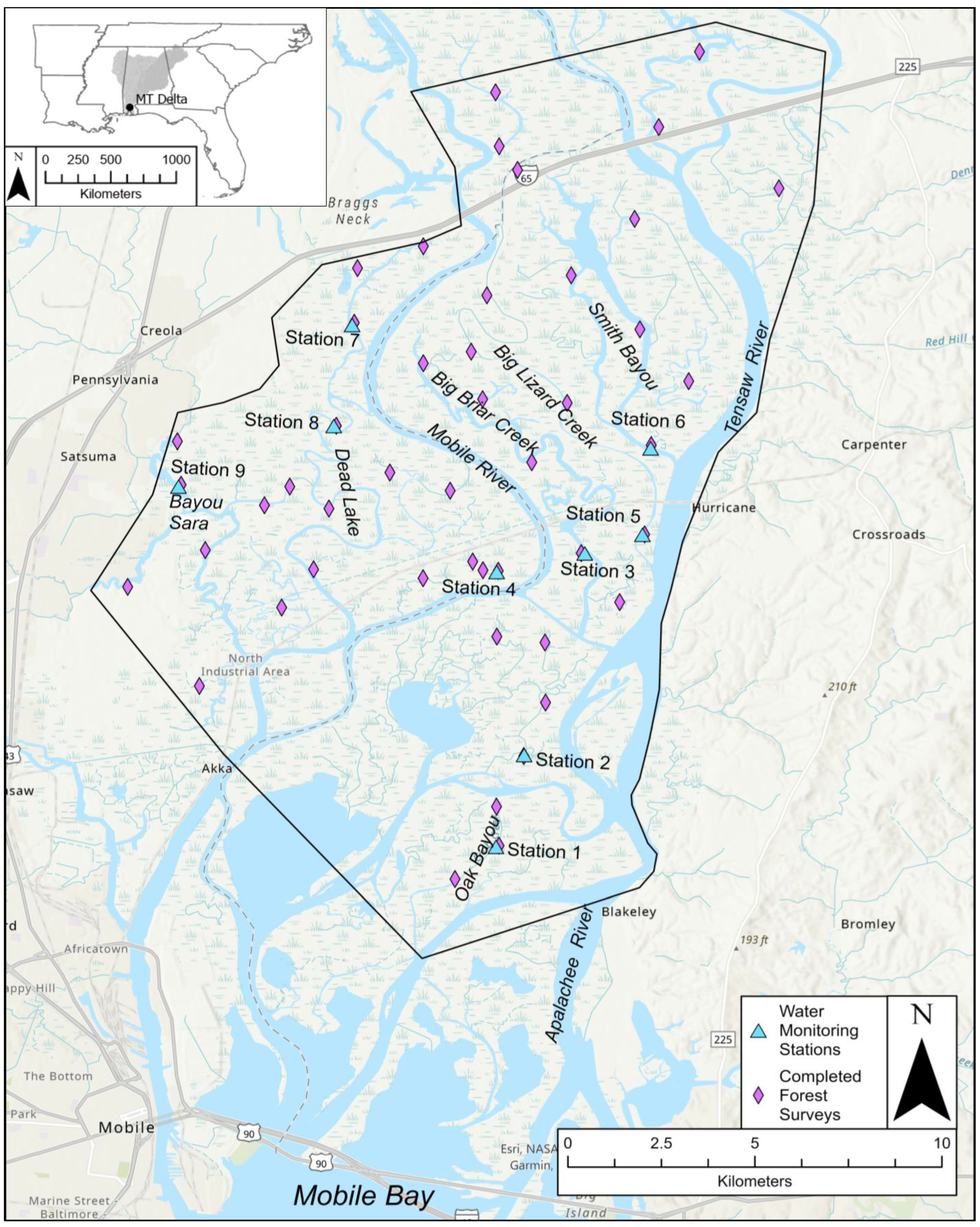
2.1. Study Site

The MT River Delta is among the largest deltas in the United States, covering an area of 140,000 ha [29]. It drains over 70% of Alabama, encompassing the Alabama, Coosa, and Tombigbee Rivers and spanning four states (Figure 1). TFFWs occupy a minimum area of ~17,000 ha throughout the lower parts of the MT River Delta. Tidal river dynamics have been documented as far upstream as 238 river kilometers (rkm) at the most seaward dams on the Alabama and Tombigbee Rivers [30], which contribute an average discharge of 900 and 850 m3/s, respectively [31,32]. The river system exhibits significant seasonal variations in total discharge, with total peak flow events reaching 15,000 m3/s during the winter/spring and exceeding 3000 m3/s during the summer/fall [30]. The estuarine input flows through shallow (3-m mean) depth Mobile Bay with the influence of diurnal microtidal (0.0–1.0 m) reach from the Gulf of Mexico. The floodplains of the MT Delta can be characterized as both red and blackwater zones, depending on the hydrologic connection of the various rivers and streams [33]. While actual soil types vary, the USDA NRCS soil map describes the study area as predominantly poorly drained wet clayey alluvial land belonging to soil group A/D or Chowan silt that is formed from woody organic material belonging to soil group B/D [34]. The area’s climate is subtropical, with a long-term average annual precipitation of 166 cm/year and average temperatures ranging from 11 to 28 °C in January and August, respectively [35]. Elevation ranges from 0.1 to 1.2 m within the forests and up to 20.1 m in the surrounding developed uplands.
Although accounts of the historical use of the MT River Delta are incomplete, the Delta has undergone significant changes over time and has been influenced by human use. It is estimated that the initial settlements in the area began around 5000 BCE, marked by the transition of transient Native American tribes to permanent river settlements driven by increased trade with other Indigenous communities [36]. Compared to other regions affected by European expansion in North America, historical records of the MT region prior to the 1700s and French settlement are relatively sparse. However, it is known that extensive timber harvesting in the MT River Delta and its floodplains began in the late 1700s. Much of this was performed by floating off-cut timber primarily around the city of Mobile by its poorer communities [37,38] and consisted of previously untouched forest habitats composed of Nyssa spp. (tupelo)/Taxodium distichum (bald cypress). Prior to the initial logging, it was estimated by early naturalist Charles Mohr that T. distichum once accounted for ~30% of all forested tree species in the entirety of the MT River Delta [25]. This was followed by a second widespread forestry operation centered around new industrial technology in the early 20th century [38]. In contrast to Mohr’s historical estimate, Aust et al. described contemporary (twice-harvested) forests in the non-tidal zone as composed of 80% N. aquatica (water tupelo) and 12% T. distichum [39].

2.2. Water Monitoring Stations

Prior to forest surveying, Solinst Levelogger 5 data loggers (n = 9) were installed in November 2021 at various tidal inlets to determine the approximate tidal reach of lower rivers in the study site (Figure 1). For each approximate location, the instruments were installed on fence posts near/at a tidal outlet draining the adjacent TFFWs. Each instrument was programmed to measure and record water level, salinity, and temperature for over two years at 15-min intervals via the Solinst level logger program. Stations were purposely staggered throughout the tidal shrub and forested zones in the lower MT River Delta to gauge tidal influence on wetland forests. A summary of water station salinity data from 2023 is provided in Table 1.

2.3. Forest Surveys

A series of forest surveys (n = 47) were conducted from March to August 2023 using 400 m2 circular plots established throughout the MT River Delta. Preliminary water data (November–March) were used as a basis for site selection (Table 1). Thus, a portion of the sampling plots (n = 27) were surveyed in proximity to the nine water monitor stations within the same water body (Figure 1). To locate the first 27 surveyed plots, nine were placed directly perpendicular (60 m) to the adjacent water monitoring station, with an additional plot placed equidistantly upstream and downstream of the station in its corresponding creek/river. The remaining plots (n = 20) were randomly spread throughout the TFFW study area to capture a range of tidal conditions, including forest management history, forested/scrub, and various water bodies. Sites were randomly selected along designated river reaches to maximize spatial variation across the tidal gradient and ultimately represent the forested tidal range along the MT River Delta.
For each plot, a center point was established, and the perimeter of the plot was flagged. Inside each plot, canopy trees with a diameter of ˃10 cm at breast height (DBH, 1.3 m high) and a total height of >15 m were identified, measured, and used to calculate species basal area (m2/ha). All subcanopy trees (defined as trees <15 m but >10 m) were identified as species and counted. Shrub/sapling individuals (defined as woody vegetation >1 m in height but not subcanopy height) were identified as species and counted. Lastly, tree health and condition assessments were conducted based on parameters from the International Society of Arboriculture Basic Tree Risk Assessment Form for all canopy trees, noting all individuals that showed evidence of stress or damage (e.g., topped branches, cavities, necrotic leaves, mistletoe, etc.) [40].

2.4. Assessment of Canopy Communities

Using forest survey data, canopy tree species’ relative density and basal area were calculated per station using the following equations:
Relative density = (no. of individuals of species x)/(no. of individuals of all species) × 100
Relative dominance = (total basal area of species x)/(total basal area of all species) × 100
The importance value (IV200), a simple statistic described by Mcintosh [41], was calculated for each species per plot. The IV200 value ranges from 0 to 200 and is defined as:
IV200 = relative density + relative dominance
Certain species, such as those in the Fraxinus (ash) genus, proved difficult to identify in the field and were therefore classified strictly at the genus level. Based on previous reports by Light et al. [42] and Anderson and Lockaby [3], we anticipated that Fraxinus trees in our study area were primarily composed of F. profunda (pumpkin ash) and F. caroliniana (Carolina ash). These species are expected to diverge along a gradient from less to more tidal conditions, respectively. Additionally, Quercus laurifolia (swamp laurel oak) and Quercus nigra (water oak) also present identification challenges due to frequent hybridization and overlapping niches, as noted in prior studies [43], and thus were also grouped at the genus level.

2.5. Multivariate Clustering Approach

Prior to clustering analysis, the rare species, Quercus lyrata (overcup oak), calculated as IV200 ≤ 19.99 in only one plot, was removed. Subsequently, IV200 values were recalculated for any plots where rare species were removed (n = 1). As the objective of the study was to characterize forest type, early successional trees, Salix nigra (black willow) and Populus heterophylla (swamp cottonwood), were manually grouped together as they both represent early successional species [44]. Additionally, four plots were removed prior to analysis because they represented shrub/scrub systems (n = 3) or were located on an atypical natural levee (n = 1). These adjustments resulted in p = 12 Species/groups prior to any statistical analysis. Next, the importance value data matrix, n43 X p12, was transformed with a Hellinger transformation using the decostand function in the R programs’ [45] vegan package [46] to eliminate 0 to 0 correlations [47,48]. Next, a Bray–Curtis dissimilarity distance matrix was analyzed using the transformed datum with the vegdist function in the vegan package [46]. All subsequent cluster-based analyses followed the techniques of Costomiris et al. [49] with the previously mentioned distance matrix and the compatible linkage method, flexible beta (β = −0.25). Clusters were then pruned from 2 to 10 levels to decipher and analyze cluster groupings of indicator species following the techniques of Dufrêne and Legendre [26] using the multiplatt function from the indicspecies package in R [50]. This resulted in an indicator value index for each species, where the indicator value index was derived from a species IV200 value association with each cluster grouping [26]. The significance of each species was assessed by comparing actual values to randomized data from 1000 Monte Carlo simulations. The total p-values for all species and the number of significant indicator species (p < 0.05) for each clustering level were subsequently recorded. Following the techniques of Dufrêne, De Câceres, and Legendre [26,50], the number of significant indicator species and their species’ respective total p-values were plotted against each cluster level (2–10), where the optimal cluster pruning (choosing the optimal number of clusters) is indicative of low total p-values and a high number of indicator species [48].
A mixed approach was used to validate the ideal cluster pruning level: the Non-metric Multidimensional Scaling (NMDS) model, the Multi-Response Permutation Procedure (MRPP) test, and indicator species analysis. The NMDS model is a technique that reduces the dimensionality of complex data sets (i.e., 2 dimensions while retaining ecological interpretation) through a non-metric nature that operates by ranking the distances between data points and then adjusting the positions of the points in a lower-dimensional space to maintain the order of distances as faithfully as possible [48]. The NMDS test was performed with the metaMDS function from the vegan package [46] with 20 real and 250 random simulations and a final stress score of a sufficient 0.16 value (<0.2). The MRPP is a non-parametric statistical test used to evaluate the significance of differences between two or more groups (clusters) of sampling units whose test statistic is based on the within-group average distance (δ) for each grouping. MRPP also generates a value of within-group agreement (homogeneity) (A), where an A value of 0 indicates no within-group homogeneity beyond random expectation, while a value of 1 indicates perfect within-group homogeneity [51]. The final validation tool was a graphical product of indicator species analysis, as described in the previous paragraph. After the initial clustering analysis, we categorized community groups into two hydrologic groups based on the clustering results and their common relationship with environmental variables. The dendrogram generated from the clustering analysis revealed distinct groupings that corresponded to relative tidal influence (supported by upriver location, station salinity, water level/tidal amplitude data, and community composition), which separated at the highest-level community groupings. By integrating the results of the clustering analysis with these environmental variables, we classified groups as either Lower Tidal or Upper Tidal.

2.6. Environmental Variables and Their Effects on Community Composition

To partially explain the between cluster dissimilarity, river distance to downstream Mobile Bay, and elevation were determined for each plot and treated as categorical variables. The river distance was calculated from aerial imagery as the shortest river distance to Mobile Bay and considered an approximate measure of tidal influence. The mean elevation was derived from the average values within each survey plot, calculated from a digital elevation model with a spatial resolution of 1 m. These two variables formed an environmental matrix of n43 X p2, which was incorporated into the NMDS models’ output in relation to their axes as biplot vectors using the envfit function from the vegan package [46]. Differences in groups were assessed with Kruskal–Wallis rank sum and Dunn’s post hoc tests (α = 0.05) [52].
To examine how river distance and elevation affect species assemblage independent of cluster designation, a Mantel Test [53] was performed using the mantel function from the vegan package [46] for each stratum, canopy, and midstory, utilizing 1000 Monte Carlo simulations. The Mantel Test evaluates whether the patterns of ecological dissimilarity (Bray–Curtis matrices of species composition) are correlated with patterns of environmental dissimilarity (Euclidean matrix from spatial components) through its’ test statistic (r), based on a scale of −1.0 to 1.0, where a value closer to −1 indicates a strong negative correlation and, in contrast, a value closer to 1 indicates a strong positive correlation [48,53]. The canopy matrix was the same as used in the cluster analysis. For the midstory stratum, rare species were removed if they occurred in <5% of plots [Carya aquatica (water hickory), Q. lyrata, Liquidambar styraciflua (sweetgum), Ilex opaca (American holly), Pinus elliottii (slash pine), and Planera aquatica (water elm)], resulting in an n43 X p21 midstory matrix. The distance matrix was also calculated using Bray–Curtis distances from Hellinger-transformed species density (m2/ha) values from the midstory matrix.

2.7. Descriptive Statistics

For each identified Community/Hydrologic Group type, we calculated various forest measures for each stratum. For the canopy stratum, we tabulated averages for basal area, species density, and proportion of stressed individuals using the mean for each value from each plot derived from species counts and DBH measurements. In the midstory stratum, common Diversity Index values, Shannon’s (H), and Species Evenness (J) were calculated for each plot [54,55] from species counts from each plot. Community statistics were calculated for each grouping’s plot mean values.

3. Results

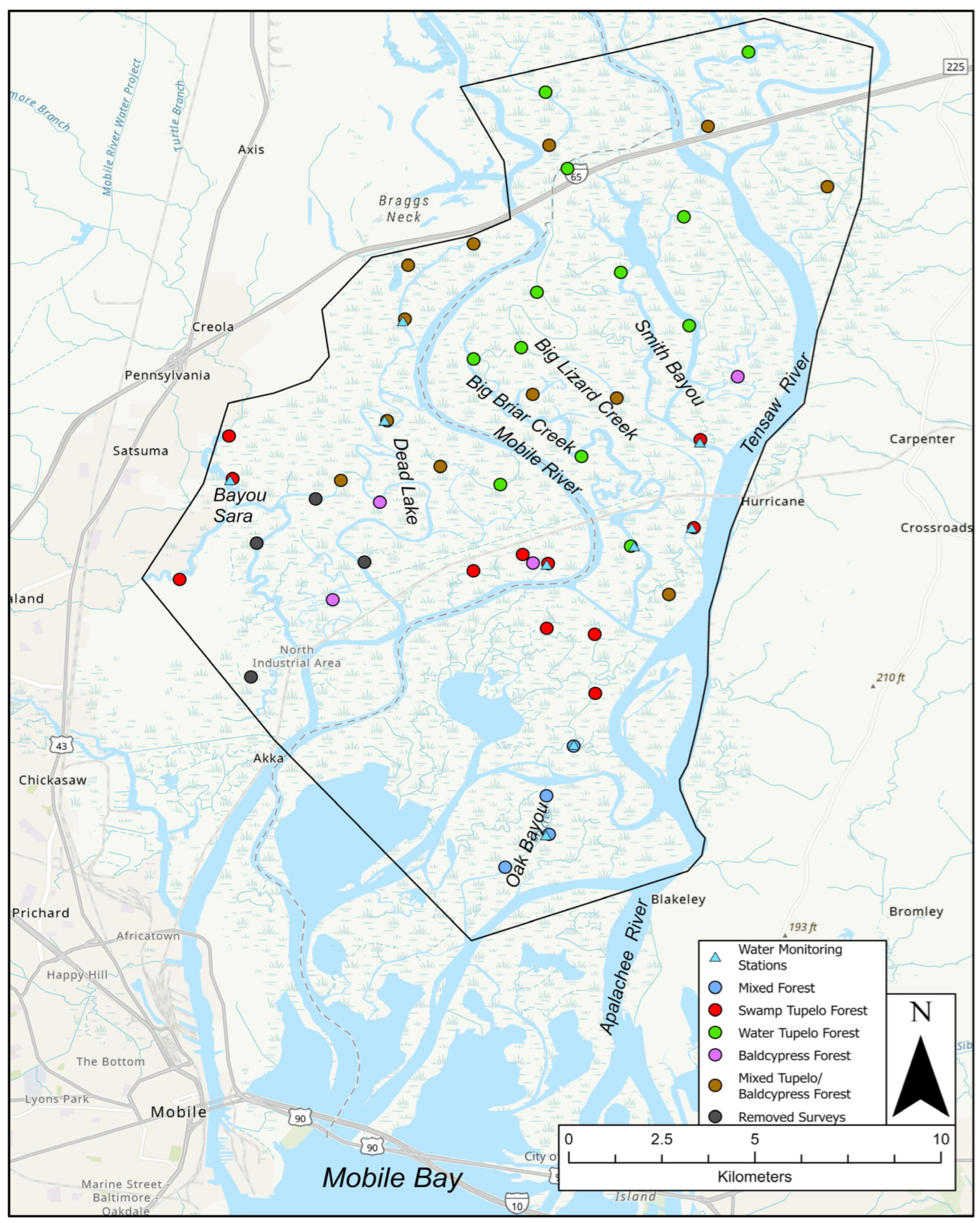
3.1. Forest Community Classification

Forest surveys yielded a wide array of forest conditions and dominant species. Canopy tree data resulted in an agglomerative coefficient of 0.89, reflecting strong and compact clusters (Figure 2) using Bray–Curtis distance and Flexible linkage (β = −0.25) methods. Pruning height was determined from the graphical product of indicator species analysis while maintaining ecological information (Figure 3), resulting in five groups of forest classifications:
(1)
Mixed Forest—Significant indicator value index species: Magnolia virginiana (sweetbay magnolia), Nyssa biflora (swamp tupelo), Fraxinus spp., and Ulmus americana (American elm).
(2)
Swamp Tupelo—Significant indicator value index species: Nyssa biflora.
(3)
Water Tupelo—Significant indicator value index species: Nyssa biflora, Nyssa aquatica, Fraxinus spp.
(4)
Bald Cypress—Significant indicator value index species: Taxodium distichum, Nyssa aquatica, and Fraxinus spp.
(5)
Bald Cypress and Mixed Tupelo—Significant indicator value index species: Nyssa biflora, Taxodium distichum, Nyssa aquatica, and Fraxinus spp.

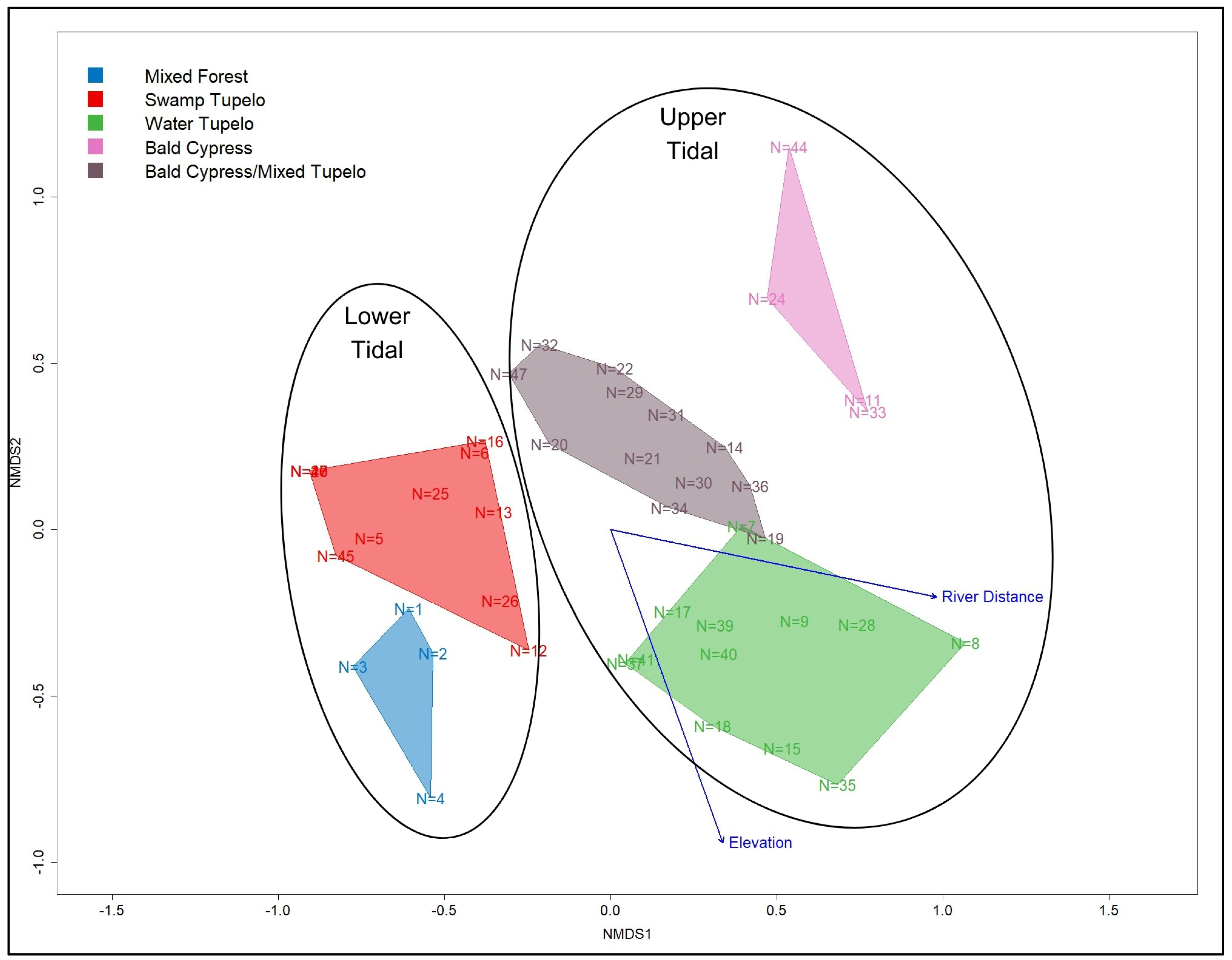
3.2. Upper and Lower Tidal Groupings

While most clusters shared a common indicator species (Table 2), the dendrogram discerned between Lower Tidal (more tidal, closer to Mobile Bay) and Upper Tidal (less tidal, further from Mobile Bay) communities among the two highest-level clusters (Figure 2), largely due to a shift in abundance of the Nyssa species (Table 2). Specifically, N. aquatica was generally absent in the Lower Tidal communities, while N. biflora was substantially less dominant in the Upper Tidal communities. These two tidal groupings were also clearly separated by their proximity to the downstream estuarine system (Table 2). Among the forest variables, the largest bifurcation between Tidal groupings was the proportion of stressed trees, with 20% of the trees in the Lower Tidal canopy showing some signs of stress, including canopy damage and infestation by Phoradendron teucrium (American mistletoe) and Agrilus planipennis (emerald ash borer) damage, compared to the Upper Tidal trees, with only 10% of individuals displaying signs of visible stress..

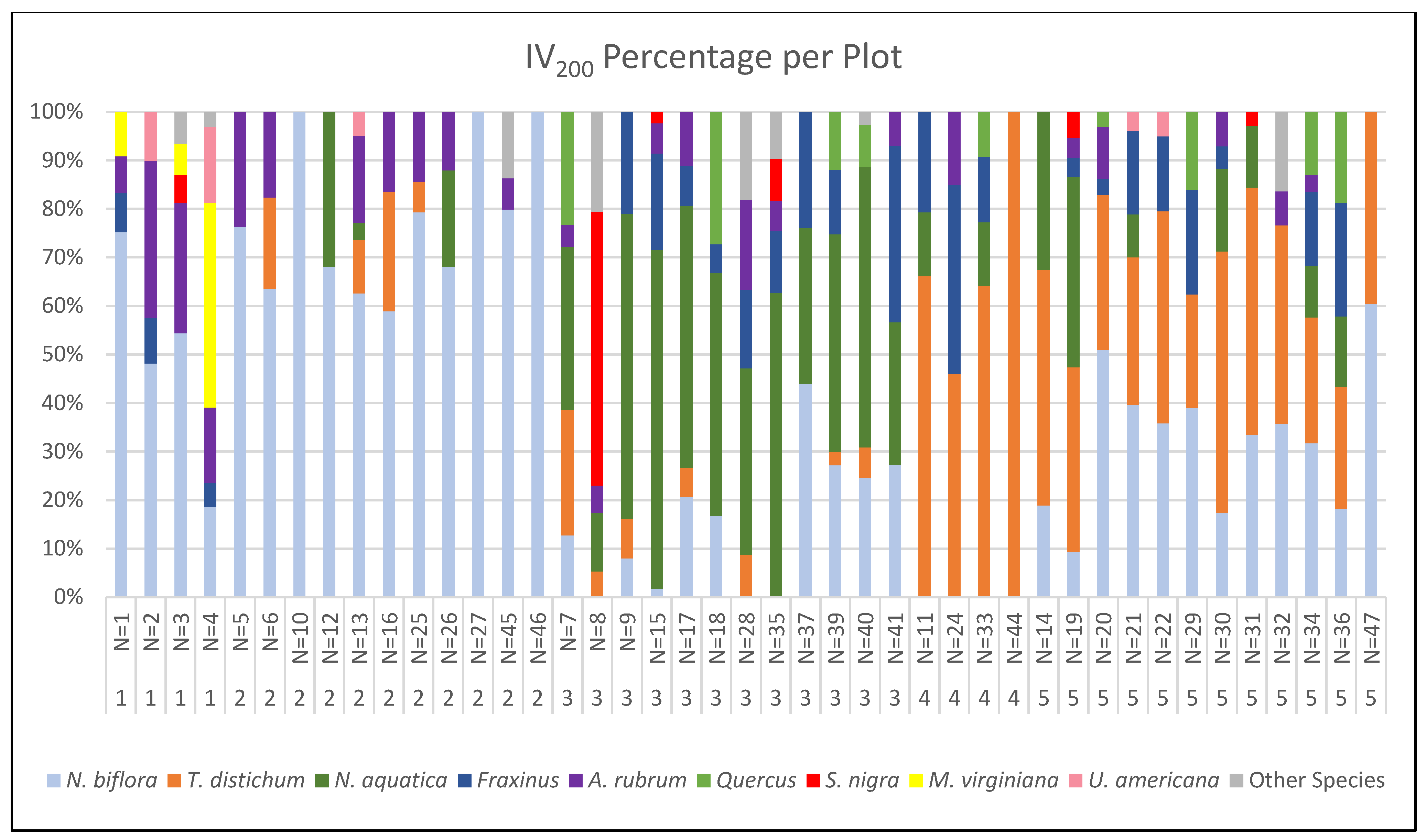
3.3. Canopy Composition across Plots

Species composition varied dramatically from plot to plot, with 14 total canopy species (Figure 4). However, particular species like N. biflora (located in 88% of plots and 40% of total IV200), T. distichum (located in 66% of plots and 19% of total IV200), and N. aquatica (located in 59% of plots and 18% of total IV200) were all widely distributed and had large comparable basal areas of the canopy trees (shown by IV200). The Mantel test showed that environmental factors had a significant moderate correlation (p = 0.001) with canopy species assemblage r = 0.26.

3.4. Relation between Environmental Variables and Forest Communities

Environmental factors of river distance (rkm) (ANOVA F = 16.6, p = 0.001) and elevation (ANOVA F = 2.5, p = 0.055) were analyzed to determine their effect on forest types. Post hoc tests showed a strong relationship with river distance (Kruskal–Wallis χ2 = 26.2, p = 0.001, df = 4), while elevation showed a similar trend with forest structure (Kruskal–Wallis χ2 = 9.0, p = 0.06, df = 4). Dunn’s test for river distance resulted in four sets of forest types having significant differences: between Mixed Forest and Water Tupelo Forests (p = 0.001), between Swamp Tupelo and Water Tupelo Forests (p = 0.004), between Bald Cypress/Mixed Tupelo and Mixed Forests (p = 0.001), and between Bald Cypress/Mixed Tupelo and Swamp Tupelo Forests (p = 0.006). Dunn’s testing for elevation differentiation between forests resulted in no statistically significant differences between forest types.
The NMDS model output exhibited optimal spacing between clusters with strong environmental vectors (Figure 5), with marginal overlapping between Bald Cypress/Mixed Tupelo and Water Tupelo forest-type polygons. While three-dimensional ordination performed more efficiently with a 0.10 stress score, we chose to use two-dimensional ordination to prioritize interpretation, which had a slightly higher stress score of 0.16 but was still under the 0.2 stress threshold. NMDS revealed that both river distance (r2 = 0.34) and elevation (r2 = 0.31) significantly correlated with the axes. Lastly, the MRPP models resulted in significantly different species compositions between the community types, A = 0.357, p = 0.001.

3.5. Midstory Composition

Midstory species varied between community types among 27 species. This is particularly noticeable in the most abundant species in the study site, Sabal minor (dwarf palm) (65.7% of the midstory), followed by Fraxinus spp. (5.7%), Morella cerifera (wax myrtle) (5.0%), and Ilex verticillata (winterberry) (4.6%) (Table 3). We noted that some species clearly separated between Upper and Lower Tidal groupings. In the Upper Tidal group, species such as I. verticillata (204 individuals/ha) and Fraxinus spp. (273 individuals/ha) were more prevalent. In contrast, M. cerifera (442 individuals/ha) and Persea palustris (swamp bay) (87 individuals/ha) are primarily present in the Lower Tidal group, whereas they are nearly absent in the Upper Tidal group (Table 3). The Mantel test shows that environmental factors have a significant correlation (p = 0.001) with midstory species assemblages r = 0.36.

3.6. Community Descriptions

Based on the results of forest surveys, cluster analyses, and other ancillary analyses, we generated a community profile for each designated TFFW community group (Figure 6).
(1)
Mixed Forest
This community was spatially concentrated in Oak Bayou, a smaller tributary of the lower Tensaw and Apalachee Rivers (Figure 6). The canopy was primarily composed of N. biflora, accounting for 49% of the IV200 in the community, followed by A. rubrum (red maple) with 21%, then M. virginiana with 13% (Figure 4: Despite having a diverse canopy community, these trees had a low relative basal area and density (compared to the Upper Tidal communities) (Table 2). The Mixed Forest also had the densest midstory but was the least diverse, almost entirely composed of S. minor, which had a density of 6144 individuals per ha (the highest density of all the community types), leading to low diversity of the overall midstory (Table 3). The Mixed Forest group had plots with the closest distance to Mobile Bay of all the forest types, with a mean distance of 11.6 rkm (Table 2). Despite being closest to the estuary, the Mixed Forest type has the second-highest mean elevation of 0.62 m (Table 2).
(2)
Swamp Tupelo Forest
The Swamp Tupelo Forest plots were spread throughout the various tributaries but restricted to the lower reaches of the study area (Figure 6). This forest type was part of the Lower Tidal communities and was characterized by its dominance of N. biflora, which accounted for 78% of the IV200 (Figure 4). The canopy community can also be characterized by its low basal area and canopy tree density (Table 2: Similar to the Mixed Forests, the midstory is heavily dominated by S. minor and M. cerifera, but with M. cerifera having a higher relative proportion of the density compared to other groups (Table 3). Additionally, the Swamp Tupelo Forest was near Mobile Bay, with a mean distance of 21.6 rkm (Table 2). The mean elevation of this forest type was 0.53 m (Table 2).
(3)
Water Tupelo Forest
The Water Tupelo Forest plots were located just upstream of the easternmost Swamp Tupelo Forests (Figure 6). It was characterized primarily by N. aquatica at 46% of the IV200, followed by N. biflora at 15% of the IV200, and Fraxinus spp. at 13% of the IV200 (Figure 4). The canopy community had a high relative basal area (second to Bald Cypress/Mixed Tupelo Forests) and the highest canopy density. The midstory was primarily composed of S. minor (the highest of the Upper Tidal communities), followed by Fraxinus spp., A. rubrum, and I. verticillata (Table 3). The diversity was relatively high but skewed due to its S. minor presence (Table 3). With a mean elevation of 0.70 m, this has the highest average elevation among forest types (Table 2). Water Tupelo Forest was considered Upper Tidal, with the longest average river distance from Mobile Bay of 32.4 rkm (Table 2).
(4)
Bald Cypress Forest
The Bald Cypress Forest plots were considered a part of the Upper Tidal area of the MT River Delta, located in a transitional zone between the Swamp Tupelo and Mixed Tupelo Baldcypress Forests (Figure 6). It was characterized by the dominance of T. distichum in the canopy, accounting for 69% of the IV200 (Figure 4), as well as both low basal area and the lowest density of all the forest types in the Delta (Table 2). The midstory was characterized by a relatively high S. minor density, followed by Fraxinus spp., I. verticillata, and T. distichum recruitment. However, for the midstory species, diversity was the lowest of the Upper Tidal forest types. Interestingly, it had the lowest average river distance from Mobile Bay, 24.3 rkm, among Upper Tidal forests (Table 2). With a mean elevation of 0.51 m, the Bald Cypress Forest type had the second lowest elevation among all forest types (Table 2).
(5)
Bald Cypress/Mixed Tupelo Forest
The Bald Cypress/Mixed Tupelo Forest plots were the most widespread surveyed forest type, located in the Upper Tidal group across a variety of tributary rivers (Figure 6). This forest was characterized by a mix of T. distichum (38% of the IV200), N. biflora (23% of the IV200), and N. aquatica (11% of the IV200) (Figure 4). The canopy was the densest and had the highest basal area of any forest type (Table 2). Its midstory was composed of S. minor (the least of any forest type), I. verticillata, and A. rubrum, with the lowest density of M. cerifera and high species diversity (Table 3). This forest type had the lowest average elevation of 0.45 m (Table 2) while having the second furthest distance to Mobile Bay among forest types of 31.5 rkm (Table 2).

4. Discussion

4.1. Community Change across a Tidal Gradient

Our results indicated that the composition and structure of TFFWs in the MT River Delta were primarily influenced by their proximity to Mobile Bay. After completion of the vegetation and water station analyses, it was noted that our study area was entirely within the tidal range of the MT River Delta. In addition to our water station data, which showed evidence of tidal hydrology, this was also supported by our canopy tree composition and hierarchical cluster analysis that differentiated in the dominance of N. aquatica, a species shown to be sensitive to saline and tidal conditions [56,57], in the forest classifications (Table 2). N. aquatica was only found in mixed composition (<50% dominance (IV200) in any forest type), compared to the 80% stem frequency reported in the forested wetlands and bottomland hardwood forests further upriver (~8 rkm) [39]. We also detected no outlier plots in the upper reaches of our study area that would indicate that conditions were shifting to non-tidal. Given that the transition between the tidal and non-tidal is gradual and imprecise [58], the detection of some N. aquatica was notable and likely represents a zone of gradual transition. Furthermore, results from the cluster analysis corresponded well with the hydrologic groupings we designated across the tidal gradient (Figure 2 and Figure 4, Figure 5 and Figure 6). The shift in community composition detected across the tidal gradient of the MT Delta was consistent with other studies conducted in the southeast United States [3,4,5,42,49,56,57,59,60,61,62,63,64,65,66], including similar ecological gradients (albeit different community types) in the Pacific Northwest [67,68] and Australia [69].
In the upper tidal reaches of the MT River Delta, canopy forest communities demonstrated a higher basal area, higher canopy density, and lower rates of visually stressed individuals (indicating a more healthy tree population) (Table 2 and Table 3). These communities primarily comprised T. distichum, N. aquatica, Fraxinus spp., and moderate occurrences of Quercus spp. and N. biflora (Table 2 and Figure 4). Many of the abovementioned species are considered sensitive to salinity exposure or sustained periods of inundation. One exception to this list is T. distichum, which generally exhibits greater tolerance to salinity and similar flood tolerance [56]. A shift between plots with less tolerant species of T. distichum was evident in the spatial distribution of the forest types (Table 2 and Figure 6), where the Bald Cypress Forest types were located closer to the bay and likely experienced higher and more frequent levels of tidal influence. Similar compositional forest types that include T. distichum have been detected in TFFWs in other studies [3,4,42,49,61,66], but our upper/lower tidal designations differed in notable ways. For instance, T. distichum was much more abundant in the lower tidal reaches of the nearby Suwanee River [42] and Apalachicola River [3]. Another potentially distinguishing characteristic of the TFFWs in the MT River Delta was the midstory stratum of the upper tidal reach, which was highly populated by S. minor, Fraxinus spp., and I. verticillata (Table 3). Absent of the S. minor, Noe et al. found similar shrub compositions (along with diversity measures) in the Upper Tidal reach of the Pamunkey River, whose canopy was primarily composed of A. rubrum and Fraxinus pennsylvanica (green ash) [66].
Lower Tidal communities of the MT Delta were characterized by lower species density, diversity, basal area, and a higher percentage of visually stressed individuals in the canopy (Table 2 and Table 3). These forests are typically located closer to the mouth of the MT Delta rivers (Table 2 and Figure 6), indicating the likely impact of more frequent and intense tidal inundation and higher salinity levels. The canopy communities are primarily composed of N. biflora (80% of the Swamp Tupelo forests and 70% of Lower Tidal forests), with some stands of M. virginiana (Table 2, Figure 4). The midstory stratum was primarily populated by S. minor and notably M. cerifera, a saline-tolerant species that can withstand periods of higher salinity (>9.0 PSU) [70] and can be commonly found in TFFWs and transitional forests [66] (Table 3). The stands of the Swamp Tupelo forests located off the Bayou Sara River likely experience sustained saltwater intrusion due to minimal river flow connections and close proximity to the bay system, as evidenced by the already transitional ghost forests at the river’s southern end (Figure 7). Although the exact mechanisms behind the creation of these ghost forests are not known, it can be expected that saltwater intrusion (evident by yearly salinity values near 2.00 PSU) (Table 1) coupled with storm impacts could have played significant roles in the vegetation dynamics, leading to the observed Cladium jamaicense (saw grass) in the exterior of the marsh and Juncus roemerianus (black needlerush) in the interior.
The mix of communities across a tidal gradient throughout various water bodies within the MT River Delta highlights the complex interplay of hydrological and environmental factors specific to each river system. Examining the spatial distribution of our plots (Figure 6), we noted distinct species composition and forest structure differences between the Mobile and Tensaw Rivers and their smaller tributaries. Most studies that characterize TFFWs (through cluster methodologies) rely on canopy tree data. However, classification based solely on canopy-level individual clustering may not account for midstory composition and, even more so, the understory. For example, many plots had extensive cover by S. minor, which made traversing these swamps difficult. However, forest classification based on canopy species would not reliably predict S. minor abundance, as we detected this species extensively across forest types. S. minor is clearly a characteristic species of the MT Delta. Moreover, only one other TFFW study has identified S. minor as an important species. While not broken down between vegetative stratums, Duberstein et al. found numerous forest stands of S. minor (with 45% of their importance value score) in the backswamps of tributary rivers of the Apalachicola River [4]. Tree canopy classification related to tidal influence may be beneficial for potential remote sensing applications. However, baseline community analysis of the midstory/understory (see Rheinhardt [59]) could better detect recent changes in tidal influence caused by sea level rise or other environmental changes, as further highlighted by the divergence Mantel’s test statistic of canopy trees (r = 0.26) and midstory vegetation (r = 0.36). Additionally, our classifications did not consistently group bivariate distributed species, I. verticillata and M. cerifera, among our forest communities but were better represented by our hydrologic characterization in the Upper and Lower Tidal groupings, respectively (Table 3). The absence of midstory strata classification poses a challenge, as understory and shrub layers can provide earlier indications of environmental shifts that are not yet apparent in the canopy.
While we found associations between our forest communities and environmental variables, there are some limitations to these variables and possible interpretations. River distance from the bay served as a proxy for tidal influence and salinity, with closer distances indicating higher tidal exposure. However, tidal conditions vary between river systems within the Delta (Table 1), and distance may not always be a good indicator. For instance, larger rivers and those with greater discharge would likely sustain less tidal influence approaching the bay than smaller rivers with less discharge [63]. Actual measures of tidal influence, including salinity and water level measures, would provide better indications of this variable. Nevertheless, between our two variables, river distance had a stronger relationship with forest type, as shown by the NMDS biplot vectors r2 = 0.34 compared to elevations’ r2 = 0.31 and the post hoc test statistics of χ2 = 26.2 and χ2 = 9.0, respectively (Figure 5). Thus, our results affirm that environmental variables (e.g. salinity) from tidal conditions are a driving factor of species biomass and assemblage in coastal tidal wetlands [61,71], thus creating the divergence between forest/hydrologic types in relation to the proximity to the estuarine input. Additionally, elevation influences the frequency and duration of flooding, with lower elevations experiencing more prolonged waterlogging, supporting species such as N. aquatica and T. distichum, which can withstand these conditions [56]. That said, relationships with both environmental variables would improve by incorporating additional plots in the non-tidal zone (i.e., swamps and bottomland forests), expanding the range of both variables, and likely improving the correlations due to the broader environmental gradients represented.

4.2. Comparing TFFWs along the Gulf of Mexico

The Suwanee and Apalachicola River Deltas are two other river systems in the northeastern part of the Gulf of Mexico comparable to the MT River Delta, which all exhibit distinct patterns of TFFW species composition and community structure across a tidal gradient. However, due to their proximity to each other, they also share some commonalities in forest structure, tidal gradient, and vulnerabilities. Light et al. reported on community characteristics of the Suwanee’s TFFWs’ vegetation, hydrology, soils, and topography [42]. While this report featured many forest types, they discerned three hydrologic groupings: Non-Tidal (dominated by T. distichum and P. aquatica), Upper Tidal (dominated by N. aquatica, T. distichum, and Fraxinus profunda), and Lower Tidal (dominated by N. biflora). They noted that Non-Tidal forests were inundated 4–7 months per year, Upper Tidal forests were flooded monthly by high tide or high river flows, and Lower Tidal forests were flooded daily or several times a month by high tides, except in isolated areas with limited connection.
The Apalachicola River Delta has been the subject of numerous studies in the past [3,4,58,63,64]. Light et al. examined the long-term stage hydrology and found the approximate boundary of tidal influence on the floodplain forests [58]. Anderson and Lockaby identified four distinct forest types throughout the tidal gradient, composed of tidal and non-tidal forests. In the tidal zone, the dominant species are N. biflora, T. distichum, Sabal palmetto (cabbage palm), and M. virginiana, compared to the non-tidal zone, which was dominated by N. aquatica, Nyssa ogeche (Ogeechee tupelo), and F. caroliniana [3]. As part of the same study, Anderson et al. found that tidal wetlands had greater tree density, larger trees were less common in tidal wetlands, the average forest basal area was significantly higher in non-tidal wetlands, and mean sapling/shrub density in tidal forests was more than twice that of non-tidal forests [64]. Celik et al. examined the difference between TFFWs in two distributary rivers of the Apalachicola River, the East River, and the St. Marks River. They found that St. Marks was the more saline closer to the bay, with a more abrupt transition to strong tidal conditions. Patterns in forest communities seemed to track the pattern in tidal influence for both rivers [52].

5. Conclusions

At the conclusion of this project, we established five distinct TFFW canopy communities in the MT River Delta that grouped into two distinct hydrologic groupings: Lower and Upper Tidal. These forest communities correlated with important environmental drivers (e.g., river distance and elevation). Our results also indicated that the Lower Tidal forests have exhibited signs of saltwater intrusion and other stressors based on evidence of lower species density, diversity, basal area, and a higher percentage of visually stressed individual trees. As this is the first comprehensive study of TFFWs conducted in the MT River Delta, additional research is necessary to assess ecosystem resilience to various stressors. This study further contributes to our understanding of TFFWs in general and the variation seen on a global extent. Moreover, future work should examine additional environmental variables and their effect on species assemblage (such as examination of the forests’ soil characteristics, hydroperiod, and flood frequency), long-term monitoring, and additional survey sites upstream of our northernmost surveys would increase spatial variability (i.e., non-tidal forests) and associated environmental variables in the MT River Delta. By further investigating the MT River Delta, we can better predict its resilience and responses to sea level rise, river flows, and other important environmental changes.

Author Contributions

Conceptualization, A.B. and C.J.A.; methodology, A.B. and C.J.A.; formal analysis, A.B., N.B. and C.J.A.; investigation, A.B.; resources, C.J.A.; data curation, A.B., N.B. and C.J.A.; writing—original draft preparation, A.B.; writing—review and editing, C.J.A. and N.B.; visualization, A.B.; supervision, C.J.A.; project administration, C.J.A.; funding acquisition, C.J.A. All authors have read and agreed to the published version of the manuscript.

Funding

This research was funded by the U.S. Department of Treasury under the Resources and Ecosystems Sustainability and Revived Economies of the Gulf Coast States Act of 2012 (RESTORE Act). This material is based upon work supported by the National Science Foundation (NSF Grant #1922687).

Data Availability Statement

The raw data supporting the conclusions of this article will be made available by the authors on request.

Acknowledgments

This project was sponsored by the U.S. Department of Treasury in cooperation with the State of Alabama Department of Conservation and Natural Resources. Kurtis Fischer, Hayden Tuite, Sam McWhorter, Brianna Travis, Kayla Boyd, Austin Stewart, Mary Hinely, Lauren Brannan. and Sam Bickley all provided field assistance. Kurtis Fischer helped with DEM mosaicking. Galen Costomiris provided advise on indicator species analysis, and Josh Goff and others at the Dauphin Island Sea Lab provided boating assistance.

Conflicts of Interest

The authors declare no conflicts of interest.

References

  1. Doyle, T.W.; O’Neil, C.P.; Melder, M.P.V.; From, A.S.; Palta, M.M. Tidal Freshwater Swamps of the Southeastern United States: Effects of Land Use, Hurricanes, Sea-Level Rise, and Climate Change. In Ecology of Tidal Freshwater Forested Wetlands of the Southeastern United States; Conner, W.H., Doyle, T.W., Krauss, K.W., Eds.; Springer: Berlin/Heidelberg, Germany, 2007; pp. 1–28. [Google Scholar] [CrossRef]
  2. Day, R.H.; Williams, T.M.; Swarzenski, C.M. Ecology of Tidal Freshwater Forested Wetlands of the Southeastern United States; Conner, W.H., Doyle, T.W., Krauss, K.W., Eds.; Springer: Berlin/Heidelberg, Germany, 2007; pp. 29–64. [Google Scholar] [CrossRef]
  3. Anderson, C.J.; Lockaby, B.G. Forested wetland communities as indicators of tidal influence along the Apalachicola River, Florida, USA. Wetlands 2011, 31, 895–906. [Google Scholar] [CrossRef]
  4. Duberstein, J.A.; Conner, W.H.; Krauss, K.W. Woody vegetation communities of tidal freshwater swamps in South Carolina, Georgia and Florida (US) with comparisons to similar systems in the US and South America. J. Veg. Sci. 2014, 25, 848–862. [Google Scholar] [CrossRef]
  5. Hackney, C.T.; Avery, G.B.; Leonard, L.A.; Posey, M.; Alphin, T. Biological, chemical, and physical characteristics of tidal freshwater swamp forests of the Lower Cape Fear River/Estuary, North Carolina. In Ecology of Tidal Freshwater Forested Wetlands of the Southeastern United States; Conner, W.H., Doyle, T.W., Krauss, K.W., Eds.; Springer: Berlin/Heidelberg, Germany, 2007; pp. 183–222. [Google Scholar] [CrossRef]
  6. Carter, V. An overview of the hydrologic concerns related to wetlands in the United States. Can. J. Bot. 1986, 64, 364–374. [Google Scholar] [CrossRef]
  7. Mitsch, W.J.; Gosselink, J.G. The value of wetlands: Importance of scale and landscape setting. Ecol. Econ. 2000, 35, 25–33. [Google Scholar] [CrossRef]
  8. Shen, X.; Jiang, M.; Lu, X.; Liu, X.; Liu, B.; Zhang, J.; Wang, X.; Tong, S.; Lei, G.; Wang, S.; et al. Aboveground biomass and its spatial distribution pattern of herbaceous marsh vegetation in China. Sci. China Earth Sci. 2021, 64, 1115–1125. [Google Scholar] [CrossRef]
  9. Letshele, K.P.; Atekwana, E.A.; Molwalefhe, L.; Ramatlapeng, G.J.; Masamba, W.R.L. Stable hydrogen and oxygen isotopes reveal aperiodic non-river evaporative solute enrichment in the solute cycling of rivers in arid watersheds. Sci. Total Environ. 2023, 859, 159113. [Google Scholar] [CrossRef] [PubMed]
  10. Anderson, C.J.; Lockaby, B.G. Seasonal patterns of river connectivity and saltwater intrusion in tidal freshwater forested wetlands. River Res. Appl. 2012, 28, 814–826. [Google Scholar] [CrossRef]
  11. Ensign, S.H.; Noe, G.; Hupp, C.R.; Skalak, K.J. Head-of-tide bottleneck of particulate material transport from watersheds to estuaries. Geophys. Res. Lett. 2015, 42, 10671–10679. [Google Scholar] [CrossRef]
  12. Brittain, R.A.; Craft, C.B. Effects of Sea-Level Rise and Anthropogenic Development on Priority Bird Species Habitats in Coastal Georgia, USA. Environ. Manag. 2012, 49, 473–482. [Google Scholar] [CrossRef] [PubMed]
  13. Korol, A.R.; Noe, G.B. Patterns of Denitrification Potential in Tidal Freshwater Forested Wetlands. Estuaries Coasts 2020, 43, 329–346. [Google Scholar] [CrossRef]
  14. Mcleod, E.; Chmura, G.L.; Bouillon, S.; Salm, R.; Björk, M.; Duarte, C.M.; Lovelock, C.E.; Schlesinger, W.H.; Silliman, B.R. A blueprint for blue carbon: Toward an improved understanding of the role of vegetated coastal habitats in sequestering CO2. Front. Ecol. Environ. 2011, 9, 552–560. [Google Scholar] [CrossRef]
  15. Adame, M.F.; Kelleway, J.; Krauss, K.W.; Lovelock, C.E.; Adams, J.B.; Trevathan-Tackett, S.M.; Noe, G.; Jeffrey, L.; Ronan, M.; Zann, M.; et al. All tidal wetlands are blue carbon ecosystems. BioScience 2024, 74, 253–268. [Google Scholar] [CrossRef] [PubMed]
  16. Costanza, R.; d’Arrée, R.; De Groot, R.; Farber, S.; Grasso, M.; Hannon, B.; Limburg, K.; Naeem, S.; O’Neill, R.V.; Paruelo, J.; et al. The value of the world’s ecosystem services and natural capital. Nature 1997, 387, 253–260. [Google Scholar] [CrossRef]
  17. Williams, T.; Amatya, D.; Connor, W.H.; Panda, S.; Xu, G.; Dong, J.; Trettin, C.; Dong, C.; Gao, X.; Shi, H.; et al. Tidal forested wetlands: Mechanisms, threats, and management tools. In Wetlands: Ecosystem Services, Restoration and Wise Use; An, S., Verhoeven, J.T.A., Eds.; Springer: Berlin/Heidelberg, Germany, 2019; pp. 129–158. [Google Scholar] [CrossRef]
  18. Grieger, R.; Capon, S.J.; Hadwen, W.L.; Mackey, B. Between a bog and a hard place: A global review of climate change effects on coastal freshwater wetlands. Clim. Chang. 2020, 163, 161–179. [Google Scholar] [CrossRef]
  19. Kirwan, M.L.; Gedan, K.B. Sea-Level Driven Land Conversion and the Formation of Ghost Forests. Nat. Clim. Chang. 2019, 9, 450–457. [Google Scholar] [CrossRef]
  20. Sweet, W.V.; Hamlington, B.D.; Kopp, R.E.; Weaver, C.P.; Barnard, P.L.; Bekaert, D.; Brooks, W.; Craghan, M.; Dusek, G.; Frederikse, T.; et al. Global and Regional Sea Level Rise Scenarios for the United States: Updated Mean Projections and Extreme Water Level Probabilities Along U.S. Coastlines; Technical Report NOS 01; National Oceanic and Atmospheric Administration, National Ocean Service (NOAA): Silver Spring, MD, USA, 2022. [Google Scholar]
  21. Field, D.W.; Reyer, A.J.; Genovese, P.V.; Shearer, B.D. Coastal Wetlands of the United States, an Accounting of a Valuable National Resource; Technical Report; National Oceanic and Atmospheric Administration: Rockville, MD, USA, 1991; p. 58. [Google Scholar]
  22. De Oliveira, G.; Lehrter, J.; Powers, S.; Mataveli, G.; Santos, C. Safely Manage Alabama’s Mobile-Tensaw Delta. Science 2024, 384, 966. [Google Scholar] [CrossRef] [PubMed]
  23. Wilson, E.O. Naturalist; Island Press: Washington, DC, USA, 2006; 416p. [Google Scholar]
  24. Bartram, W. The Travels of William Bartram; University of Georgia Press: Athens, GA, USA, 1998; 824p. [Google Scholar]
  25. Mohr, C. Plant life of Alabama. An Account of the Distribution, Modes of Association, and Adaptations of the Flora of Alabama, Together with a Systematic Catalogue of the Plant Growing in the State; Brown Printing Co.: Montgomery, AL, USA, 1901; 137p. [Google Scholar]
  26. Dufrêne, M.; Legendre, P. Species assemblage and indicator species: The need for a flexible asymmetrical approach. Ecol. Monogr. 1997, 67, 345–366. [Google Scholar] [CrossRef]
  27. Brown, J.H. On the relationship between abundance and distribution of species. Am. Nat. 1984, 124, 255–279. [Google Scholar] [CrossRef]
  28. Malik, R.N.; Husain, S.Z. Linking remote sensing and ecological vegetation communities: A multivariate approach. Pak. J. Bot. 2008, 40, 337–349. [Google Scholar]
  29. Szabo, M.W.; Osborne, E.W.; Copeland, C.W., Jr.; Neathery, T.L. Geologic Map of Alabama; Special Map 220; Geological Society of Alabama: Tuscaloosa, AL, USA, 1988. [Google Scholar]
  30. Dykstra, S.L.; Dzwonkowski, B. The propagation of fluvial flood waves through a backwater-estuarine environment. Water Resour. Res. 2020, 56, e2019WR025743. [Google Scholar] [CrossRef]
  31. U.S. Geological Survey. National Water Information System; USGS Water Data for the Nation. Location ID 02428400. 2016. Available online: https://waterdata.usgs.gov/monitoring-location/02428400/ (accessed on 1 June 2024).
  32. U.S. Geological Survey. National Water Information System; USGS Water Data for the Nation. Location ID 02469761. 2016. Available online: https://waterdata.usgs.gov/monitoring-location/02469761/ (accessed on 1 June 2024).
  33. Waselkov, G.A.; Andrus, C.F.; Plumb, G.E. A State of Knowledge of the Natural, Cultural, and Economic Resources of the Greater Mobile-Tensaw River Area; Natural Resource Report NPS/NRSS/BRD/NRR—2016/1243; Biological Resources Division, National Park Service: Fort Collins, CO, USA, 2016.
  34. U.S. Department of Agriculture, Natural Resources Conservation Service. Soil survey of Mobile County, Alabama. Available online: https://www.nrcs.usda.gov/wps/portal/nrcs/main/soils/survey/ (accessed on 29 April 2024).
  35. National Centers for Environmental Information. U.S. Climate Normals, Monthly Normals, Station USW00013894, Alabama. Available online: https://www.ncei.noaa.gov/access/us-climate-normals/#dataset=normals-monthly&timeframe=15&location=AL&station=USW00013894 (accessed on 17 July 2024).
  36. Ensor, H.B.; Wilson, E.M.; Hill, M.C. Historic Resources Assessment, Tennessee-Tombigbee Waterway Wildlife Mitigation Project, Mobile and Tensaw River Deltas, Alabama; COESAM/PDER-93-002; Panamerican Consultants Inc.: Tuscaloosa, AL, USA, 1993; 80p. [Google Scholar]
  37. Weaver, D.C. Cultural Resources Reconnaissance Study of the Black Warrior-Tombigbee System Corridor, Alabama; DACWOI-8 1-C-OOO1; University of South Alabama: Mobile, AL, USA, 1983; Volume III. [Google Scholar]
  38. Mader, S.F. Recovery of Functions and Plant Community Structure by a Tupelo-Baldcypress Wetland Ecosystem following Timber Harvesting. Ph.D. Thesis, College of Forest Resources, North Carolina State University, Raleigh, NC, USA, 1990. [Google Scholar]
  39. Aust, W.M.; Fristoe, T.; Gellerstedt, P.; Giese, L.; Miwa, M. Long-term effects of helicopter and ground-based skidding on site properties and stand growth in a tupelo-cypress wetland. Ecol. Manag. 2006, 226, 72–79. [Google Scholar] [CrossRef]
  40. Matheny, N.; Clark, J. A photographic Guide to the Evaluation of Hazard Trees in Urban Areas; International Society of Arboriculture: Savoy, IL, USA, 1994; 84p. [Google Scholar]
  41. Mcintosh, R.P. The York Woods: A Case History of Forest Succession in Southern Wisconsin. Ecology 1957, 38, 29. [Google Scholar] [CrossRef]
  42. Light, H.M.; Darst, M.R.; Lewis, L.J.; Howell, D.A. Hydrology, Vegetation, and Soils of Riverine and Tidal Floodplain Forests of the Lower Suwannee River, Florida, and Potential Impacts of Flow Reductions; 1656A; US Geological Survey: Reston, VA, USA, 2002.
  43. Burk, C.J. The Hybrid Nature of Quercus laurifolia. J. Elisha Mitchell Sci. Soc. 1963, 79, 159–163. [Google Scholar]
  44. Keeland, B.D.; Gorham, L.E. Delayed tree mortality in the Atchafalaya Basin of southern Louisiana following Hurricane Andrew. Wetlands 2009, 29, 101–111. [Google Scholar] [CrossRef]
  45. R Core Team. R: A Language and Environment for Statistical Computing; R Foundation for Statistical Computing: Vienna, Austria, 2021; Available online: https://www.R-project.org/ (accessed on 27 March 2024).
  46. Oksanen, J.; Blanchet, F.G.; Friendly, M.; Kindt, R.; Legendre, P.; McGlinn, D.; Minchin, P.R.; O’Hara, R.B.; Simpson, G.L.; Solymos, P.; et al. Vegan: Community Ecology Package. Version 2.6. 2024. Available online: https://CRAN.R-project.org/package=vegan (accessed on 27 March 2024).
  47. Legendre, P.; De Cáceres, M. Beta diversity as the variance of community data: Dissimilarity coefficients and partitioning. Ecol. Lett. 2013, 16, 951–963. [Google Scholar] [CrossRef] [PubMed]
  48. McCune, B.; Grace, J.B. Analysis of Ecological Communities; MjM Software Design: Gleneden Beach, OR, USA, 2002; Volume 28, 300p. [Google Scholar]
  49. Costomiris, G.; Hladik, C.M.; Craft, C. Multivariate Analysis of the Community Composition of Tidal Freshwater Forests on the Altamaha River, Georgia. Forests 2024, 15, 200. [Google Scholar] [CrossRef]
  50. De Câceres, M.; Legendre, P. Associations between species and groups of sites: Indices and statistical inference. Ecology 2009, 90, 3566–3574. [Google Scholar] [CrossRef] [PubMed]
  51. Mielke, P.W. 34 Meteorological applications of permutation techniques based on distance functions. In Handbook of Statistics, 1st ed.; Krishnaiah, P.R., Sen, P.K., Eds.; Elsevier: Amsterdam, The Netherlands, 1984; Volume 7, pp. 813–830. [Google Scholar]
  52. Dunn, O.J. Multiple comparisons using rank sums. Technometrics 1964, 6, 241–252. [Google Scholar] [CrossRef]
  53. Mantel, N.A. The detection of disease clustering and a generalized regression approach. Cancer Res. 1967, 27, 209–220. [Google Scholar] [PubMed]
  54. Shannon, C.E. A mathematical theory of communication. Bell Syst. Tech. J. 1948, 27, 379–423. [Google Scholar] [CrossRef]
  55. Pielou, E.C. The measurement of diversity in different types of biological collections. J. Theor. Biol. 1966, 13, 131–144. [Google Scholar] [CrossRef]
  56. Connor, W.H.; Krauss, K.W.; Doyle, T.W. Ecology of Tidal Freshwater Forests in Coastal Deltaic Louisiana and Northern South Carolina. In Ecology of Tidal Freshwater Forested Wetlands of the Southeastern United States; Conner, W.H., Doyle, T.W., Krauss, K.W., Eds.; Springer: Berlin/Heidelberg, Germany, 2007; pp. 223–253. [Google Scholar] [CrossRef]
  57. Penfound, W.T.; Hathaway, E.S. Plant communities in the marshlands of southeastern Louisiana. Ecol. Monogr. 1958, 8, 3–5. [Google Scholar] [CrossRef]
  58. Light, H.M.; Vincent, K.R.; Darst, M.R.; Price, F.D. Water-Level Decline in the Apalachicola River, Florida from 1954 to 2004, and Effects on Floodplain Habitats; USGS Scientific Investigations Report 2006–5173; U.S. Geological Survey: Reston, VA, USA, 2006.
  59. Rheinhardt, R. A Multivariate Analysis of Vegetation Patterns in Tidal Freshwater Swamps of Lower Chesapeake Bay, USA. Bull. Torrey Bot. Club 1992, 119, 192–207. [Google Scholar] [CrossRef]
  60. Duberstein, J.; Kitchens, W. Community composition of select areas of tidal freshwater forest along the Savannah River. In Ecology of Tidal Freshwater Forested Wetlands of the Southeastern United States; Springer: Berlin/Heidelberg, Germany, 2007; pp. 321–348. [Google Scholar] [CrossRef]
  61. Krauss, K.W.; Duberstein, J.A.; Doyle, T.W.; Conner, W.H.; Day, R.H.; Inabinette, L.W.; Whitbeck, J.L. Site condition, structure, and growth of bald cypress along tidal/non-tidal salinity gradients. Wetlands 2009, 29, 505–519. [Google Scholar] [CrossRef]
  62. Liu, X.; Conner, W.H.; Song, B.; Jayakaran, A.D. Forest composition and growth in a freshwater forested wetland community across a salinity gradient in South Carolina, USA. Forest Ecol. Manag. 2017, 389, 211–219. [Google Scholar] [CrossRef]
  63. Celik, S.; Anderson, C.J.; Kalin, L.; Rezaeianzadeh, M. Long-term salinity, hydrology, and forested wetlands along a tidal freshwater gradient. Estuaries Coasts 2021, 44, 1816–1830. [Google Scholar] [CrossRef]
  64. Anderson, C.J.; Lockaby, B.G.; Click, N. Changes in Wetland Forest Structure, Basal Growth, and Composition across a Tidal Gradient. Am. Midl. Nat. 2013, 170, 1–13. [Google Scholar] [CrossRef]
  65. Conner, W.; Whitmire, S.; Duberstein, J.; Stalter, R.; Baden, J. Changes within a South Carolina Coastal Wetland Forest in the Face of Rising Sea Level. Forests 2022, 13, 414. [Google Scholar] [CrossRef]
  66. Noe, G.B.; Bourg, N.A.; Krauss, K.W.; Duberstein, J.A.; Hupp, C.R. Watershed and estuarine controls both influence plant Community and tree growth changes in tidal freshwater forested wetlands along two US Mid-Atlantic Rivers. Forests 2021, 12, 1182. [Google Scholar] [CrossRef]
  67. Janousek, C.N.; Folger, C.L. Variation in Tidal Wetland Plant Diversity and Composition Within and among Coastal Estuaries: Assessing the Relative Importance of Environmental Gradients. J. Veg. Sci. 2014, 25, 534–545. [Google Scholar] [CrossRef]
  68. Johnson, L.K.; Simenstad, C.A. Variation in the Flora and Fauna of Tidal Freshwater Forest Ecosystems Along the Columbia River Estuary Gradient: Controlling Factors in the Context of River Flow Regulation. Estuaries Coasts 2015, 38, 679–698. [Google Scholar] [CrossRef]
  69. Grieger, R.; Capon, S.J.; Hadwen, W.L.; Mackey, B. Spatial Variation and Drivers of Vegetation Structure and Composition in Coastal Freshwater Wetlands of Subtropical Australia. Mar. Freshw. Res. 2021, 72, 1746–1759. [Google Scholar] [CrossRef]
  70. Sande, E.; Young, D.R. Effect of sodium chloride on growth and nitrogenase activity in seedlings of Myrica cerifera L. New Phytol. 1992, 120, 345–350. [Google Scholar] [CrossRef]
  71. Crain, C.M.; Silliman, B.R.; Bertness, S.L.; Bertness, M.D. Physical and Biotic Drivers of Plant Distribution across Estuarine Salinity Gradients. Ecology 2004, 85, 2539–2549. [Google Scholar] [CrossRef]
Figure 1. The lower Mobile-Tensaw River Delta study site with completed forest surveys, water monitoring station locations, and the watershed, where the black-lined outline denotes the study site.
Forests 15 01359 g001
Figure 2. Dendrogram from Hellinger transformed canopy tree data with a Bray–Curtis distance matrix and Flexible linkage (β = −0.25), analyzed with 12 species/groupings from 43 forest plots. Groupings are defined by different colored lines, with the pruning height being the dashed black line.
Forests 15 01359 g002
Figure 3. Graphical representation of indicator species analysis for each cluster, ranging from 2 to 10 clusters (x-axis). An indicator value was used for all 12 species/groups against cluster level, where the subsequent p-values were extracted from the Monte Carlo simulations and their values summed (z-axis) along with the number of significant indicator species, p < 0.05 (y-axis). The vertical dashed red line at k = 5 indicates the final pruning point.
Forests 15 01359 g003
Figure 4. Plot-level species IV200 for all clustered forest plots. Bars represent the cumulative percentage IV200 of all species in each plot. The bottom number represents forest type based on clustering: (1) Mixed Forest, (2) Swamp Tupelo, (3) Water Tupelo, (4) Bald Cypress, and (5) Bald Cypress and Mixed Tupelo.
Forests 15 01359 g004
Figure 5. NMDS ordination of plots separated by cluster in two dimensions. Significant (<0.05) environmental vector overlay indicates the relationship of elevation in meters and river distance to plot ordination. Circles indicate tidal grouping.
Forests 15 01359 g005
Figure 6. Spatial orientation of cluster-based forest types and long-term water monitoring stations.
Forests 15 01359 g006
Figure 7. Ghosts forest of the MT River Delta, composed of standing dead T. distichum trees throughout a Cladium jamaicense marsh, located at the downstream extent of the Bayou Sara Tributary.
Forests 15 01359 g007
Table 1. Water monitoring station mean and maximum salinity for 2023 (1 January–31 December).
Monitoring StationMean Salinity (PSU)Max Salinity (PSU)
Station 11.5314.06
Station 21.4912.26
Station 31.0310.33
Station 41.0514.66
Station 50.242.88
Station 60.234.56
Station 70.263.61
Station 80.465.79
Station 91.749.71
Table 2. Mean IV200 (±1 SE) for canopy trees in each forest type and hydrologic group. Bold numbers represent significant indicator value index species by classification.
Forest TypeHydrologic Group
SpeciesMixed Forest (n = 4)Swamp Tupelo (n = 11)Water Tupelo (n = 12)Bald Cypress (n = 4)Bald Cypress/Mixed Tupelo (n = 12)Lower Tidal (n = 15)Upper Tidal (n = 28)
Acer rubrum41.1 (6.0) 19.8 (5.4)10.3 (3.4)7.5 (5.8)5.4 (2.2)25.5 (5.3)7.8 (2.0)
Fraxinus spp.11.2 (3.3)-26.4 (6.4)36.6 (12.6)17.4 (5.2)3.0 (1.7)24.0 (4.2)
Nyssa aquatica-10.1 (6.5)92.2 (9.5)13.1 (5.9)22.6 (7.6)7.4 (4.8)51 (8.6)
Nyssa biflora98.2 (18.1)155.7 (9.5)30.4 (8.1)-65.0 (8.5)140 (11.2)40.9 (6.6)
Persea palustris1.6 (1.2)2.5 (2.5)---2.2 (1.8)-
Quercus lauriflora/nigra--11.9 (5.7)4.6 (3.6)8.5 (4.2)-8.7 (3.1)
Taxodium distichum-11.0 (5.3)10.9 (4.3)138.1 (17.5)75.4 (6.0)8.1 (4.1)56.7 (6.9)
Ulmus americana12.9 (6.0)0.9 (0.9)--1.5 (1.0)4.1 (2.4)0.6 (0.4)
Magnolia virginiana28.9 (14.6)----7.7 (5.7)-
Populus heterophylla--5.9 (4.5)---2.5 (2.0)
Salix nigra2.9 (2.2)-9.3 (7.5)-1.4 (1.0)0.8 (0.8)5.2 (3.3)
Triadica sebifera3.3 (2.5)-2.2 (2.2)-2.7 (2.7)0.9 (0.9)2.1 (1.5)
Forest/Environmental Variables
Mean basal area (m2/ha)17.2 (3.7)14.3 (3.8)31.8 (3.9)15.9 (4.4)32.9 (4.5)15.0 (3.0)30.0 (2.8)
Mean density (no./ha)363 (36)266 (44)475 (68)181 (47)379 (38)292 (36)392 (38)
Proportion of stressed trees (%)20 (10)21 (7)14 (0)16 (7)5 (2)20 (10)10 (0)
Mean river distance (rkm)11.6 (1.2)21.6 (1.0)32.4 (1.9)24.3 (1.9)31.5 (1.8)18.9 (1.4)30.9 (1.2)
Mean elevation (m)0.62 (0)0.53 (0.1)0.70 (0)0.51 (0.1)0.45 (0.1)0.5 (0.0)0.6 (0.0)
Table 3. Mean (±1 SE) species’ density (No. of individuals/ha) of midstory species between community type and hydrologic groups.
Forest TypeHydrologic Group
SpeciesMixed
Forest
(n = 4)
Swamp Tupelo
(n = 11)
Water
Tupelo
(n = 12)
Bald Cypress (n = 4)Bald Cypress/Mixed
Tupelo (n = 12)
Lower Tidal
(n = 15)
Upper Tidal (n = 28)
Sabal minor6144 (984)2330 (567)2052 (599)2544 (907)1369 (485)3347 (679)1829 (352)
Persea palustris113 (46)77 (40)-44 (34)6 (4)87 (34)9 (6)
Acer rubrum188 (92)193 (40)167 (67)63 (26)127 (38)192 (38)135 (33)
Morella cerifera313 (97)489 (210)38 (31)44 (34)17 (12)442 (169)29 (15)
Cephalanthus occidentalis19 (6)80 (22)50 (28)44 (21)65 (31)63 (19)55 (18)
Cornus foemina6 (6)23 (13)8 (6)--18 (11)4 (3)
Ilex cassine44 (16)23 (10)--6 (6)28 (9)3 (3)
Ilex vomitoria38 (22)18 (9)-6 (5)4 (4)23 (9)3 (2)
Ilex verticillata-102 (57)150 (87)119 (80)288 9175 (47)204 (56)
Quercus lauriflora/nigra-21 (11)35 (21)19 (15)46 (23)15 (9)38 (13)
Ulmus americana6 (6)2 (2)21 (11)-25 (14)3 (2)20 (8)
Triadica sebifera6 (6)5 (4)2 (2)-35 (20)5 (4)16 (9)
Salix nigra13 (13)39 (15)6 (6)13 (10)4 (3)32 (13)6 (3)
Nyssa biflora31 (12)150 (55)50 (10)63 (37)44 (15)118 (46)49 (10)
Populus heterophylla-16 (15)38 (31)-29 (27)12 (12)29 (17)
Nyssa aquatica-25 (18)54 (25)6 (5)60 (35)18 (15)50 (18)
Taxodium distichum-20 (7)33 (8)81 (57)50 (31)15 (6)47 (16)
Itea virginica-89 (59)15 (9)19 (9)77 (35)65 (48)42 (16)
Planera aquatica--6 (6)-4 (4)-4 (3)
Baccharis halimifolia-34 (23)---25 (19)-
Fraxinus spp.13 (7)102 (35)325 (92)512 (153)142 (54)78 (29)273 (57)
Species diversity (H)0.5 (0.2)1.2 (0.1)1.1 (0.1)0.9 (0.1)1.3 (0.1)1.0 (0.1)1.1 (0.1)
Species evenness (J)0.2 (0.1)0.6 (0.1)0.5 (0.1)0.5 (0.1)0.6 (0.1)0.5 (0.1)0.6 (0)
Disclaimer/Publisher’s Note: The statements, opinions and data contained in all publications are solely those of the individual author(s) and contributor(s) and not of MDPI and/or the editor(s). MDPI and/or the editor(s) disclaim responsibility for any injury to people or property resulting from any ideas, methods, instructions or products referred to in the content.

