Association of Carbon Pool with Vegetation Composition along the Elevation Gradients in Subtropical Forests in Pakistan

Abstract

As the most important way to mitigate climate change, forest carbon storage has been the subject of extensive research. A comprehensive study was carried out to investigate the influence of elevation gradients and diameter classes on the forest growth, composition, diversity, and carbon pools of the Bagh Drush Khel Forest area. Research revealed that elevation gradients significantly influenced the composition, diversity, and carbon pools in forests. At lower elevations, Eucalyptus camaldulensis was the dominant species, with Olea ferruginea as a co-dominant species, whereas at higher elevations, Pinus roxburghii was the dominant species with Quercus incana as a co-dominant species. Regeneration was higher at higher elevations with the maximum number of saplings and seedlings of P. roxburghii. Species diversity association with elevation was negative (R² = −0.44; p < 0.05—Shannon Index). Soil organic carbon (SOC association with elevation was non-significant while positive with DBH classes (R² = 0.37; p < 0.05). Overall, carbon pool association with elevation and diameter at breast height (DBH) were negative (R² = −0.73; p < 0.05) and (R² = −0.45; p < 0.05). Litter biomass correlated positively with elevation (R² = 0.25; p < 0.05) and DBH (R² = 0.11; p < 0.05), while deadwood biomass correlated negatively with elevation gradients (R² = −0.25; p < 0.05), and no effect was observed for DBH classes. The highest carbon stock (845.89 t C/ha) was calculated at low elevations, which decreased to (516.27 t C/ha) at high elevations. The overall carbon stock calculated was (2016.41 t C/ha) respectively. A total of six tree species were found at the study site. Future research is essential for forest health monitoring and understanding fine-scale impacts. This study offers a methodological framework for similar investigations in unexplored yet potentially significant forest regions worldwide.

1. Introduction

Carbon sequestration and biodiversity protection are two of the most significant worldwide environmental benefits of forests, and they are currently hot topics [1]. With 861 ± 66 Pg of carbon stored worldwide, forests are a key source of carbon storage, with 44% of the carbon being in the soil (up to a depth of 1 m) and 42% being in live biomass [2], dead organic stuff, such as dead wood and litter, contains the remaining portion [3]. Since the creation and execution of the program for reduced emissions from deforestation and forest degradation (REDD+), the forest carbon store has been the subject of extensive research [1].

A variety of factors, such as forest types [4,5], regeneration mode [6], age or successional stage of the forest [7], and tree diversity and density [8,9], can affect above-ground tree biomass (AGTB) [10]. Similarly, soil organic carbon (SOC) is impacted by factors like above-ground litterfall and root turnover [11], temperature and precipitation [12], soil conditions and vegetation type [13], species diversity and richness [14], soil properties and soil moisture [15], altitude [16], slope aspect and soil depths [17].

The seemingly opposing association between the diversity of tree species and soil and biomass carbon is an intriguing observation [9]. Multiple soil-related and climate-related variables impact forest carbon storage [18]. Additionally, temperature, precipitation, atmospheric pressure, solar radiation, wind speed, and other environmental parameters significantly vary with altitude [19]. With increasing altitude, the carbon pool in living biomass decreases [20]. Forest inventories often include surveys to evaluate the forests’ characteristics efficiently [21]. First, scientists at the first stages determine the taxonomic and ecological composition of forest stand for various further aims [22,23]. The two main elements of biodiversity are species richness and diversity, which are crucial for managing and conserving forests. The stability of ecosystems and the form and function of forests are directly related to them [24]. Most evaluations of species richness include the nature of the area as a primary consideration [25], and as elevation rises, species richness generally tends to decrease [25]. However, the availability of space for high mountain plants to grow varies throughout time [26].

In Pakistan, only 5.01% (4.54 million ha) of the land comprises forests and planted trees [27]. Most lie in the northern territories [28,29,30,31]. Many studies have been conducted to assess the forest biomass and carbon stock in the northern territory [32,33,34,35,36,37]. In the northwest of Pakistan, Khyber Pakhtunkhwa has 1.504 million hectares of forest [28,29], which was the transitional zone between Pakistan’s two predominant forest ecosystems: the subtropical broadleaved evergreen and subtropical Chir pine forests; it makes up around one-third of all the country’s wooded territory, with a significant portion of its natural forests [33]. The assessment of species diversity and carbon pools in this context has not been explored. The terrain characteristics of the region, such as significant differences in altitude and abundant tree species, make it a typical area for research, while knowledge of the effects of elevation gradients and diameter classes on forest biomass, species diversity, and soil-litter-deadwood capacity to sequester carbon in Bagh Drush Khel, Swat, is poorly documented.

Therefore, to address all these issues, a comprehensive study has been conducted in Bagh Drush Khel, Swat region, to evaluate the influence of elevation and diameter classes on tree growth, species diversity, and carbon pool. We hypothesized that the elevation gradient significantly influences various aspects of forest ecosystems, including tree growth rates, diameter class distribution, regeneration status, species diversity, and soil carbon accumulation, with complex and interconnected relationships shaping the overall dynamics of forest ecosystems along elevational gradients.

The primary objectives of this study were to (i) quantify tree biomass and carbon stock across three distinct diameter classes at varying elevation gradients; (ii) to assess the regeneration status of various tree species at different elevation gradients; (iii) to evaluate tree species diversity across different elevation gradients; (iv) to measure litter and deadwood carbon stock within the three specified diameter classes across varying elevation gradients; and (v) to determine soil organic carbon (SOC) stock for soil depths of 0–20 cm and 21–40 cm within the three diameter classes at different elevation gradients.

2. Materials and Methods

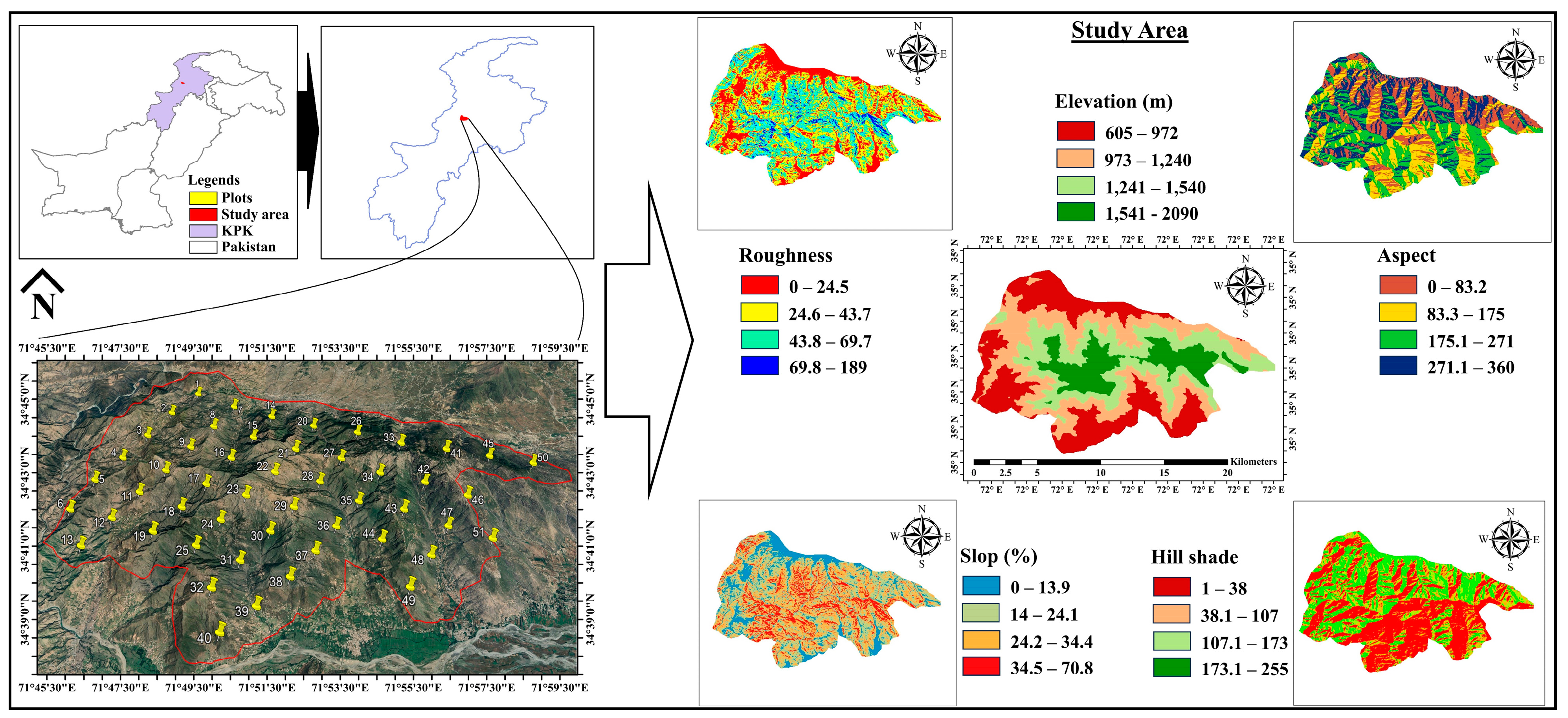
2.1. Study Area

The study was conducted in the Bagh Drush Khel, Swat district, Khyber Pakhtunkhwa, northern Pakistan ‘Figure 1’. Swat is a mountainous green valley between 34°51′ N 71°51′ E. Swat District has boundaries with Swat District to the east, Upper Dir District to the north, Malakand and Bajaur District to the south, and Afghanistan to the west. The region has significant variations in temperature throughout the year, even within the same month at various locations. At Bagh Drush Khel, the mean maximum temperature in June is 32.8 °C, while the average minimum temperature in January is 2.9 °C at the same location [38]. Bagh Drush Khel’s yearly average rainfall is 112.7 mm respectively ‘

Table 1. Climatic features of the study area.

Months	Temperature °C			Ppt mm	Humidity %
	Max.	Min.	Avg.		Max.	Min.	Avg.
January	11.58	0.9	6.24	70.67	48.21	28.88	38.55
February	12.68	2.7	7.69	207.7	60.32	40.23	50.28
March	17.53	6.95	12.24	178.24	58.32	39.23	48.78
April	23.47	11.73	17.60	150.35	53.43	36.61	45.02
May	29.5	16.49	23.00	81.01	45.43	23.32	34.38
June	32.48	20.43	26.46	66.7	42.82	22.59	32.71
July	31.1	21.81	26.46	250.48	68.34	39.74	54.04
August	28.32	18.93	23.63	255.65	82.67	46.98	64.83
September	26.13	15.13	20.63	85.86	67.11	40.01	53.56
October	22.39	10.89	16.64	45.42	47.11	27.18	37.15
November	17.05	5.47	11.26	52.19	44.4	23.08	33.74
December	13.86	2.32	8.09	28.05	40.01	18.01	29.01

’. The elevation range varies between 600–2100 m (msl).

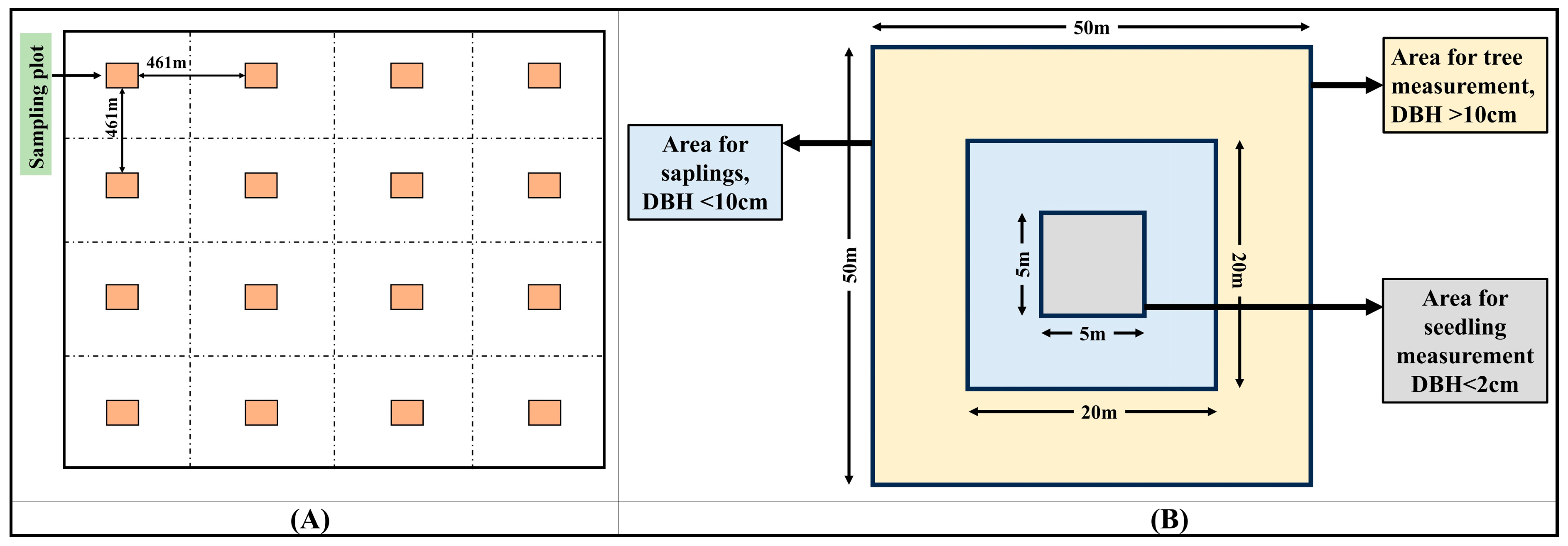
2.2. Sampling and Inventory

The field inventory was conducted from 10 July–10 September 2022. The sampling area containing two major forest types: subtropical broadleaved and Subtropical Chir-Pine. Three elevation gradients were formulated based on elevation: E1 = 800–1166 m (Low), E2 = 1167–1533 m (Middle), and E3 = 1534–1900 m (High); 17 sampling plots of (50 × 50 m—each) were taken for each elevation gradient. A GPS device was used to mark each sampling plot’s positioning accurately. Three diameter classes were constructed: DBH-class I = <25 cm, DBH-class II = 25–40 cm, and DBH-class III = >40 cm. Using a systematic sampling method based on the Fishnet tool in ArcGIS version 10.8, 51 sampling plots were taken to invent the 1085 ha area ‘Figure 2A’. The DBH of trees >10 cm was measured in a 50 m square plot. The number of stems for smaller tree saplings of DBH < 10 cm was measured in a 20 m square plot, and the number of seedlings DBH < 2 cm was measured in a 5 m square plot ‘Figure 2B’. Five quadrats (1 × 1 m—each), one in the center and the remaining four on each corner of the square plot were taken in each (50 × 50 m) sampling plot to calculate litter, deadwood, soil biomass, and carbon stock.

2.2.1. Litter Sampling

The leaves and litter from the 1 × 1 m subplots were gathered and weighed fresh. To calculate total dry mass and organic matter, 100 g of equally mixed sub-samples were placed in a polythene bag and brought to the lab to measure the moisture content [39,40].

2.2.2. Deadwood Sampling

When calculating deadwood biomass, standing dead wood with branches was measured using a method equivalent to the allometric equation for estimating biomass above ground; however, if the dead wood measured <1.3 m in height, its diameter and height were measured as near the top as possible and classified as a logged tree [41]. There was a 2%–3% deduction for hardwood/broadleaved species and 5%–6% for soft-wood/conifer species from their branches when standing dead wood was devoid of leaves [40,41].

2.2.3. Soil Sampling

To determine SOC, soil samples from the top 30 cm layer were taken using a soil auger. Since most of the SOC is located here, samples taken at this depth are sufficient, according to IPCC [42]. Shallow soils and rocks below the surface make it challenging to gather samples from a depth of more than 30 cm [33].

2.3. Biomass Calculation

2.3.1. Tree and Sapling Biomass

In each sampling plot, the DBH and height of each tree (DBH > 10 cm) and sapling (DBH < 10) were measured using a Vernier caliper (Haglof Sweden AB, Klockargatan 8, Långsele, Sweden) and Spiegel relay scope (Carl Zeiss AG, Carl-Zeiss-Straße 22, Oberkochen, Germany). The basal area and tree volume of each tree were calculated using the equations proposed by Khan et al. [32]. Above-ground biomass was calculated using the allometric equations as presented in

Table 2. Allometric equations used to calculate the above-ground biomass of six different tree species.

Tree Species	Allometric Equation	Reference
Eucalyptus camaldulensis	$AGB=0.023\times {[D^2\times H]}^{0.9985}$	[43]
Acacia modesta	$AGB=0.2267\times {[D^2\times H]}^{0.8226}$	[32,44]
Olea ferruginea	$AGB=7.8863+0.0556\times [D^2\times H]$	[32,44]
Melia azedarach	$AGB=-5.7225+2.0365\times \ln [D^2\times H]$	[45]
Pinus roxburghii	$AGB=0.0224\times {[D^2\times H]}^{0.9767}$	[43]
Quercus incana	$AGB=0.8277\times {[D^2\times H]}^{0.6655}$	[32]

.

Where, AGB = above-ground biomass in kg, D = dia at breast height in cm, and H = tree height in m.

Whereas (Equation (1)) was used to calculate sapling above-ground biomass [46].

$$\log AGSB=a+b\log (D)$$

(1)

where, AGSB = above-ground sapling biomass in kg, D = dia at breast height in cm, a = intercept of allometric relationship for saplings [dimensionless], and b = slope allometric relationship for saplings [dimensionless].

After calculating the above-ground biomass of the tree, below-ground biomass was calculated using the root-to-shoot ratio (R) conversion method by multiplying above-ground biomass with 0.2 [32]. Total tree biomass was calculated by summing above and below-ground biomass [35]. For tree carbon stock calculations, total tree biomass was multiplied with a conversion factor of 0.47 [32,33,34,35,36].

2.3.2. Litter Biomass

Following laboratory work, the appropriate allometric equation was used to compute the carbon stock in tons/ha for each plot. Following Pearson et al. [41] (Equations (2) and (3)) were used to calculate litter biomass and carbon stock.

$$LB={\displaystyle \frac{W_{field}}{A}}\times {\displaystyle \frac{W_{sub-sample(dry)}}{W_{sub-sample(fresh)}}}\times {\displaystyle \frac{1}{10,000}}$$

(2)

$$C_L=LB\times C_{\%}$$

(3)

where, LB = Litter biomass t/ha); W_field = weight of fresh field sample of litter sampled within an area of size (g); A = size of the area in which litter was collected (ha); W_{sub-sample(dry)} = weight of the oven-dry sub-sample, W_{sub-sample(fresh)} = weight of the fresh sub-sample of litter taken to the laboratory to determine moisture content (g), C_L = total carbon stocks in the dead litter t/ha, C_% = carbon fraction determined in the laboratory [41].

2.3.3. Deadwood Biomass

Since most of the current species (except Pinus roxburghii) are broadleaved, estimations of the deadwood carbon stock might be obtained by subtracting two to three percent from each tree’s total above-ground biomass. The allometric equation (Equation (4)) was validated in the REDD approach to calculate the biomass value in standing dead wood [40,41]. Total deadwood biomass was calculated using (Equation (5)); furthermore, to calculate deadwood carbon stock, total deadwood biomass was multiplied by a conversion factor of 0.47.

$$SDWB={\displaystyle {\sum }_{i=0}^n\frac{1}{3}}\times {[D/200]}^2\times h\times s$$

(4)

$$DW{B}_T=SDW{B}_{Branched}+SDW{B}_{non-branched}$$

(5)

where, SDWB = standing deadwood biomass (kg), h = length (m), D = tree diameter (cm), s = specific gravity (g/cm³) of wood [value of s was used as 0.5 g/cm³ as suggested by Hairiah et al. [47], DWB_T = Total Deadwood biomass, SDWB_Branched = standing deadwood biomass of branched wood, and SDWB_non-branched = standing deadwood biomass of non-branched wood.

2.3.4. Soil Biomass

The soil’s bulk density and carbon content were estimated using a composite sample approach [39]. Bulk density is the dry weight of a unit volume of soil. The assessment of bulk density considers both solid particles and pore spaces and is impacted by several factors, like the amount of organic matter present, the degree of compaction, and the consolidation of particles—low soil bulk density results from high organic matter [48].

A digital balance was used on the spot to measure the samples’ moist weights. Following transportation to the Pakistan Forest Institute, samples were sealed in polythene bags, permitted to air dry, and then placed in the oven for 24 h at 105 °C to remove all moisture from the soil. The dehydrated samples’ moisture content (M_C%) was calculated using Equation (6) [49].

$$M_C\%={\displaystyle \frac{W_w-W_d}{W_d}}\times 100$$

(6)

where, M_C (%) = moisture content, Ww = wet weight, and W_d = dry weight.

The samples were cleared of stones, and the net weights were noted. The soil auger’s diameter and length were measured to calculate its volume. Bulk density was computed using Equation (7) [50].

$$B_D={\displaystyle \raisebox{1ex}{$W_d$}\!\left/ \!\raisebox{-1ex}{$V_s$}\right.}$$

(7)

where BD = bulk density, W_d = oven dry weight of the sample (g), and Vs = volume of soil core (cm³).

The loss on ignition (LoI) approach was used to quantify the soil’s organic matter [50]. A china dish with a 50 g sample of dried soil was put in a muffle stove with a temperature of 400 °C. The samples were burned to ash by running the furnace nonstop for 8 h. Equation (8) was utilized to calculate each sample’s organic matter content, and the ash’s weight was documented [51].

$$O_M=W_d-W_a$$

(8)

where O_M = organic matter (g), W_d = weight of the oven-dried sample (g), Wa = weight of ash (g).

The soil organic carbon (SOC) amount was computed using a factor of 0.58 [51]. The soil carbon density, or SOC per hectare, for each elevation gradient, was calculated using Equation (9) [42].

$$SOC=\rho \times d\times C\times 100$$

(9)

where SOC = soil organic carbon, ρ = the soil bulk density, d = soil sample depth, and C = carbon content in the sample.

2.4. Species Dominance

Using the importance value index (IVI), the species dominance of each DBH class at each elevation gradient was determined. The dominant species was determined to have the highest important value, while the co-dominant species was defined as the one with the second highest value. The relative frequency, relative density, and relative dominance percentage counts were added together to create this index, and the final result was assigned the species’ IVI (Equations (10)–(13)). The relative frequency, density, and basal area values for each species in different size classes were calculated to determine the IVI in different elevation gradients, following Curtis and McIntosh [52] and Chapagain et al. [53].

$$RelativeFrequency(RF)={\displaystyle \frac{Frequencyofaspecies}{Totalfrequencyofallspecies}}\times 100$$

(10)

$$Relative Density(RD)={\displaystyle \frac{Sumofindividualsofaspecies}{Totalcountofallindividuals}}\times 100$$

(11)

$$RelativeDominance(RDom)={\displaystyle \frac{Sumofdominanceofaspecies}{Totaldominanceofallspecies}}\times 100$$

(12)

$$IVI=RF+RD+RDom$$

(13)

Relative density, relative frequency, and relative basal area added up to the IVI for trees and saplings, whereas relative density and relative frequency added up to the IVI for seedlings [53]. The effect of elevation gradient on trees, saplings, and seedlings of different tree species in three DBH classes was analyzed by examining their densities per plot. A linear Regression model was used to find the association of IVI values of each DBH class’s trees, saplings, and seedlings with elevation gradient. Furthermore, IVI per DBH class of each species was subjected to two-way ANOVA following elevation gradient. Similarly, Tukey’s multiple comparison test was used to compare the mean difference at a 5% significance level.

2.5. Vegetation Diversity

Alpha diversity was investigated at the plot level to measure variety within the localized overstory community. This approach to determining the richness of a particular forest ecosystem component is widespread [54,55] and helpful considering the diversity of overstory tree species that support different kinds of wildlife.

Alpha diversity was determined using four indices: Species richness, which is determined as the number of distinct species in the plot; Shannon-wiener diversity index (Equation (14)) [56]; Pielou’s evenness index (Equations (15) and (16)) [57], and Simpson Index (Equations (17) and (18)) [58].

Shannon-wiener diversity index

$$H\prime =-{\displaystyle {\sum }_{n=1}^s{p}_i}\ln p_i$$

(14)

where, S is species richness, pi is the proportion of each species in the sample, and ln is the natural log.

Pielou’s evenness index

$$J\prime ={\displaystyle \frac{H\prime }{H_{max}^{\prime }}}$$

(15)

$$H_{max}^{\prime }=-{\displaystyle {\sum }_{i=1}^s\frac{1}{s}}\ln {\displaystyle \frac{1}{s}}$$

(16)

Simpson Diversity index

$$D={\displaystyle \frac{1}{{\displaystyle {\sum }_{i=1}^{s}p{i}^2}}}$$

(17)

$$\begin{array}{l}\mathrm{Gini}\text{-}\mathrm{Simpson}\mathrm{index}=(1-D)\\ =1-\left({\displaystyle \frac{{\displaystyle \sum n_i(n_i-1)}}{N(N-1)}}\right)\end{array}$$

(18)

where p is the proportion (n/N) of individuals of one particular species found (n) divided by the total number of individuals found (N), Σ is still the sum of the calculations, and “s” is the number of species.

A linear regression model was used to determine the association between species diversity and elevation gradient. Furthermore, diversity indices per plot were subjected to one-way ANOVA following the elevation gradient. Similarly, Tukey’s multiple comparison test was used to compare the mean difference at a 5% significance level.

2.6. Carbon Pool Calculation

The overall carbon pool at each elevation gradient for each DBH class was calculated by summing the carbon stock densities of the individual carbon pools using Equation (19) [41]. Each variable value was calculated by summing the values of each DBH class for each elevation gradient.

$$C_{density}=C_{AGB}+C_{BGB}+C_{SB}+C_L+C_{Dw}+SOC$$

(19)

where C_density = Carbon stock density for all pools (t C ha⁻¹), C_AGB = carbon in above-ground tree biomass (t C ha⁻¹], C_BGB = carbon in below-ground tree biomass (t C ha⁻¹), C_SB = carbon in sapling biomass (t C ha⁻¹), C_L = carbon in dead litter (t C ha⁻¹), C_Dw = carbon in dead wood biomass (t C ha⁻¹), and SOC = Soil organic carbon (t C ha⁻¹).

2.7. Statistical Analysis

Descriptive statistics of stem density (trees/ha), DBH (cm), tree height (m), basal area (m²/ha), and volume (m³/ha) by DBH class intervals and elevation gradients were calculated to summarize. All the variables were tested for normality and heterogeneity of the variance using the Shapiro-Wilk normality test (p-value > 0.05) and Levene’s test (p-value > 0.05). Multiple Linear Regression (MLR) was employed to determine if there was any significant association between mean stem density, height, basal area, volume, and biomass of six tree species from three DBH classes with elevation gradients. All these variables per plot were subjected to two-way ANOVA following the elevation gradient and DBH class intervals. Similarly, Tukey’s multiple comparison test was used to compare the mean difference at a 5% significance level. A correlation model was used to calculate whether there was any significant association between different carbon pools with DBH classes and elevation gradients. These analyses were performed using IBM SPSS Statistics version-26, and graphs and figures were created using Microsoft Office Excel-365.

3. Results

3.1. Characteristics of Stands at Different Elevations

Association of species composition with elevation gradients was significant and correlated negatively (F = 4.91, Adj. R² = −0.10, p < 0.05) ‘

Table 3. Effect of elevation gradients on the forest growth parameters, assessed by Linear Regression model.

Fixed Variable	Growth Variables	Unstandardized Coefficients		Standardized Coefficients
		B	S.E	Beta	t	Sig.	Adj. R2	F-Value
Elevation Gradient	Spp. C	−0.42	0.19	−0.16	−2.90	0.03	−0.10	4.91
	SD	−1.43	0.11	−0.41	−13.64	0.00	−0.41	186.01
	DBH	0.34	0.59	0.02	0.57	0.56	0.02	0.33
	TH	0.21	0.15	0.04	1.38	0.16	0.05	1.92
	BA	−0.55	0.09	−0.20	−6.27	0.00	−0.20	39.32
	Vol	−1.39	0.41	−0.11	−3.39	0.00	−0.11	11.48
	TB	−56.15	4.16	−0.41	−13.49	0.00	−0.40	181.99

Spp. C = Species composition, SD = Stand density, DBH = Diameter at breast height, TH = Tree height, BA = Basal area, Vol = Tree Volume, TB = Tree Biomass.

’. At lower elevations, species composition was high, with E. camaldulensis as a dominant species, compared to the high elevation with P. roxburghii. The association of stand density with elevation gradients was significant and correlated negatively (F = 186.01, Adj. R² = −0.41, p < 0.05). The highest stand density was recorded (6.36 ± 0.54 trees/ha) for DBH class-I at low elevation and gradually decreased to (1.72 ± 0.19 trees/ha) for DBH class-III at high elevation ‘

Table 4. Distribution of DBH, tree density, height, basal area, volume, above and below-ground biomass, tree biomass, and tree CS of the forest concerning elevation gradients and DBH classes. Values are represented as (Mean ± SE).

Elevation Gradients	DBH Classes	No. of Trees	DBH (cm)	Height (m)	BA (m2/ha)	Vol (m3/ha)	AGB (t/ha)	BGB (t/ha)	TB (t/ha)	CS (t C/ha)
Low	I	6.36 ± 0.54	19.16 ± 0.53	7.42 ± 0.19	1.76 ± 0.12	4.43 ± 0.34	209.88 ± 18.12	41.98 ± 3.62	251.86 ± 21.75	125.93 ± 10.87
	II	4.46 ± 0.38	29.12 ± 0.83	10.23 ± 0.15	2.86 ± 0.22	9.78 ± 0.82	143.74 ± 12.52	28.75 ± 2.50	172.49 ± 15.02	86.24 ± 7.51
	III	3.53 ± 0.30	44.13 ± 0.64	12.54 ± 0.14	5.30 ± 0.40	22.15 ± 1.67	109.86 ± 9.32	21.97 ± 1.86	131.83 ± 11.18	65.92 ± 5.59
Middle	I	4.19 ± 0.50	19.42 ± 0.81	7.66 ± 0.31	1.38 ± 0.16	3.82 ± 0.47	137.50 ± 16.64	27.50 ± 3.33	165.00 ± 19.97	82.50 ± 9.98
	II	3.06 ± 0.40	30.81 ± 1.55	9.99 ± 0.36	2.48 ± 0.31	8.88 ± 1.15	97.70 ± 13.01	19.54 ± 2.60	117.24 ± 15.61	58.62 ± 7.81
	III	2.25 0.25	46.16 ± 1.64	12.67 ± 0.45	4.17 ± 0.44	18.73 ± 1.94	69.12 ± 7.60	13.82 ± 1.52	82.94 ± 9.12	41.47 ± 4.56
High	I	2.26 ± 0.20	19.11 ± 0.37	7.29 ± 0.17	0.94 ± 0.10	2.78 ± 0.34	73.77 ± 6.58	14.75 ± 1.32	88.52 ± 7.89	44.26 ± 3.95
	II	2.06 ± 0.21	31.03 ± 0.93	9.43 ± 0.13	2.22 ± 0.21	8.42 ± 0.83	64.92 ± 6.57	12.98 ± 1.31	77.90 ± 7.89	38.95 ± 3.94
	III	1.72 ± 0.19	42.98 ± 0.69	11.88 ± 0.23	3.56 ± 0.34	17.13 ± 1.53	52.55 ± 5.86	10.51 ± 1.17	63.06 ± 7.03	31.53 ± 3.51

DBH = Dia at breast height, BA = Basal area, Vol = Tree Volume, AGB = Above ground biomass, BGB = Below ground biomass, TB = Tree Biomass, CS = Tree carbon stock.

’.

The highest tree density (10.42 ± 0.90 trees/ha) was recorded for Eucalyptus camaldulensis at low elevation for DBH class I, while at high elevation for all DBH-classes, no tree was found for Eucalyptus. At middle and high elevations for DBH class II and III, the highest value was recorded for Olea ferruginea (3.61 ± 0.55, and 2.56 ± 0.24 trees/ha) ‘Table S1’. The association of DBH with elevation gradients was non-significant, and weak positive correlated was observed (F = 0.33, Adj. R² = 0.02, p > 0.05) ‘Table 3’. The highest DBH was recorded (46.16 ± 1.64 cm) for DBH class-III at the middle elevation, whereas the lowest value (19.11 ± 0.37 cm) was recorded for DBH class-I at the high elevation ‘Table 4’. The highest DBH was recorded at higher elevation for Pinus roxburghii ‘Table S1’. The association between tree height and elevation gradients was also non-significant, while a weak positive correlation exists among them (F = 1.92, Adj. R² = 0.05, p > 0.05) ‘Table 3’. At high elevations, low tree height was recorded (7.29 ± 0.17 m) for DBH class-I compared to middle and low elevations; however, the highest tree height recorded (12.67 ± 0.45 m) was recorded at middle elevation for DBH class-III ‘Table 4’.

For DBH class-I, maximum height was recorded for Q. incana at high elevation, and lowest was observed for Acacia modesta at low elevation. This pattern of height gradually increased with an increase in DBH and elevation. For DBH class III at high elevation, the highest value was observed for Pinus roxburghii ‘Table S1’. Basal area (BA) association with elevation gradient was significantly correlated negatively (F = 39.32, Adj. R² = −0.20, p < 0.05) ‘Table 3’. The highest basal area was recorded (5.30 ± 0.40 m²/ha) for DBH class-III at low elevation, while the lowest BA was observed (0.94 ± 0.10 m²/ha) for DBH class-I at high elevation ‘Table 4’. The maximum value of the basal area was observed for Pinus roxburghii from DBH class I at high elevation, whereas the minimum value of the basal area was observed for Melia azedarach from DBH class I at high elevation. Elevation gradients and tree volume association were significantly correlated negatively (F = 11.48, Adj. R² = −0.11, p < 0.05). The highest tree volume was observed (22.15 ± 1.67 m³/ha) for DBH class-III at low elevation, and the lowest tree volume value was calculated as (2.78 ± 0.34 m³/ha) for DBH class-I at high elevation. At a high elevation for DBH class III, the maximum tree volume was observed for P. roxburghii, while the minimum tree volume was observed for Melia azedarach from DBH class I. Tree biomass was significantly correlated negatively with elevation gradients (F = 181.99, Adj. R² = −0.40, p < 0.05) ‘Table 3’. At low elevation, the highest tree biomass value (251.86 ± 21.75 t/ha) was recorded for DBH class-I, and at high elevation, a low tree biomass value (63.06 ± 7.03 t/ha) was observed for DBH class-III ‘Table 4’. The highest tree biomass and tree carbon stock values were observed for Eucalyptus camaldulensis from DBH class I at E1, whereas the lowest values were observed for Melia azedarach from DBH class III at E3, respectively ‘Table S1’.

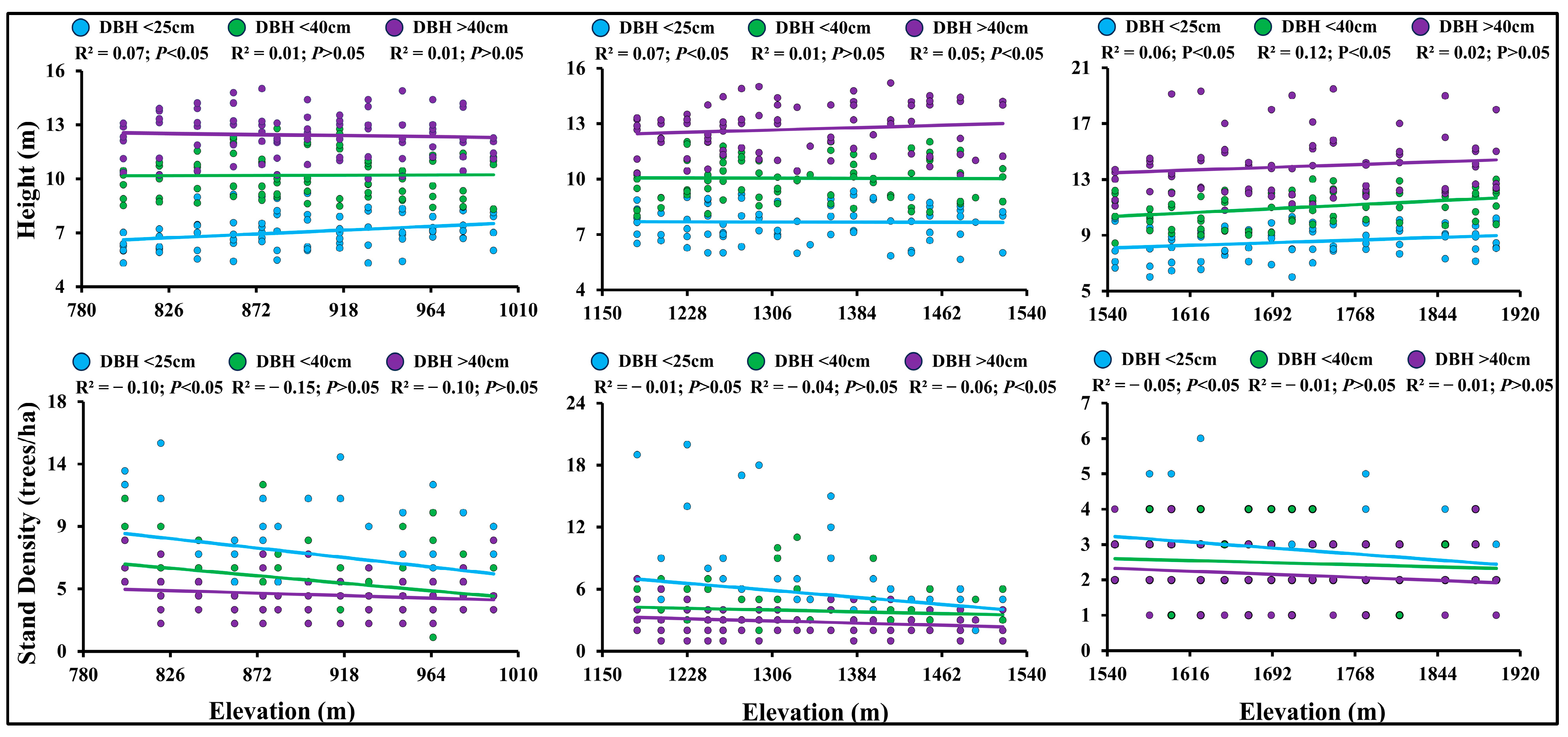
3.2. Association of Tree Height and Density of Different DBH Classes with Elevation

On the plot scale level, elevation gradients significantly influence the tree height and stand density of all tree species from three different DBH classes [F (2, 872) = 1.23, p < 0.01]. Tree height of trees having DBH < 25 cm was only influenced significantly by low elevation (R² = 0.07; p < 0.05); for middle elevation, the height of trees having DBH > 40 cm was only significantly influenced by elevation (R² = 0.05; p < 0.05); and at high elevation, the height of tree having DBH < 25 and <40 influenced significantly by elevation (R² = 0.06 and R² = 0.12; p < 0.05) ‘Figure 3’. For stand density, all diameter class trees at low elevation were significantly influenced by elevation (p < 0.05) and correlated negatively with the highest correlation value (R² = −0.15; p < 0.05) for trees having DBH < 40 cm, while trees with DBH > 40 cm at middle elevation and <25 cm at high elevation significantly influenced by elevation (R² = −0.06 and R² = −0.05; p < 0.05).

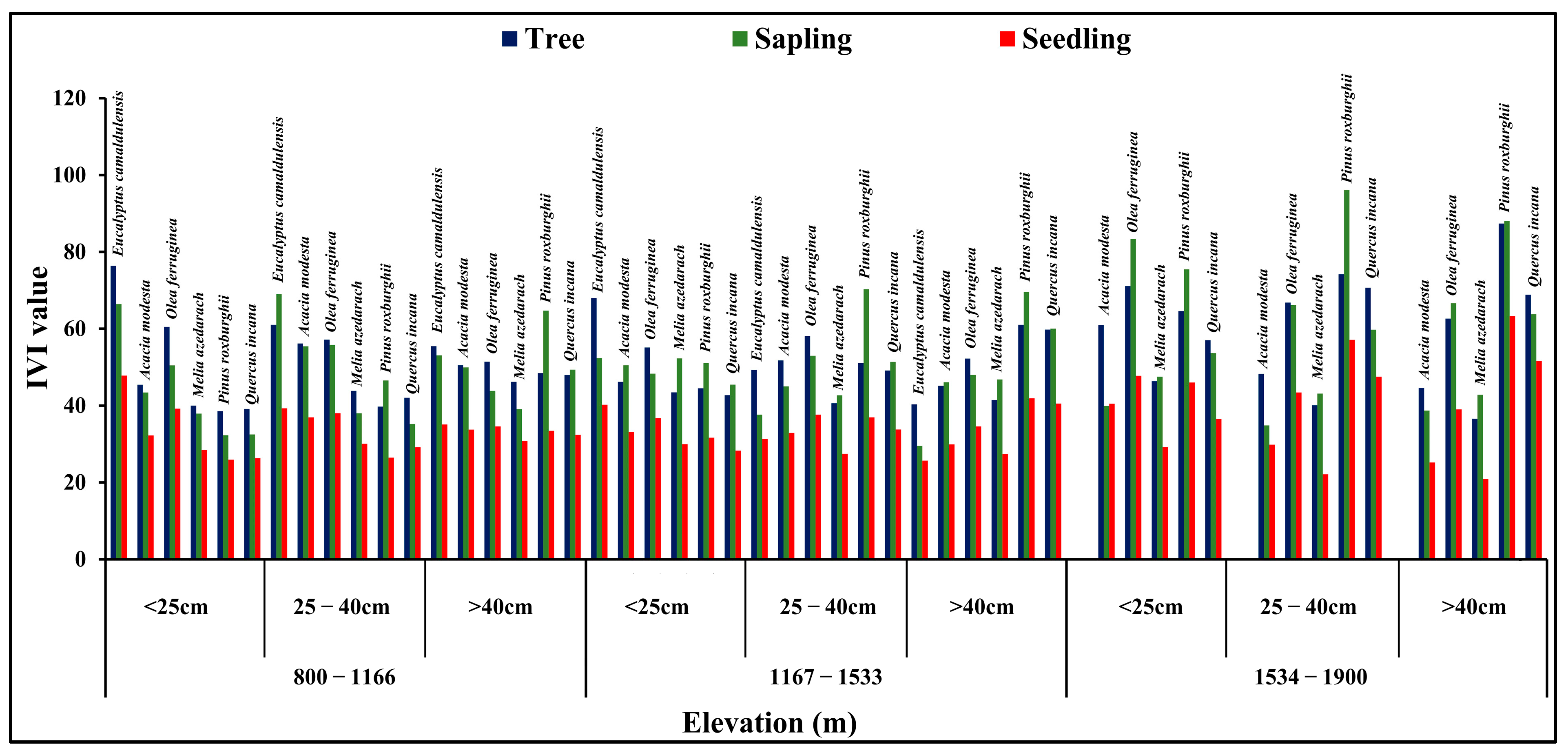
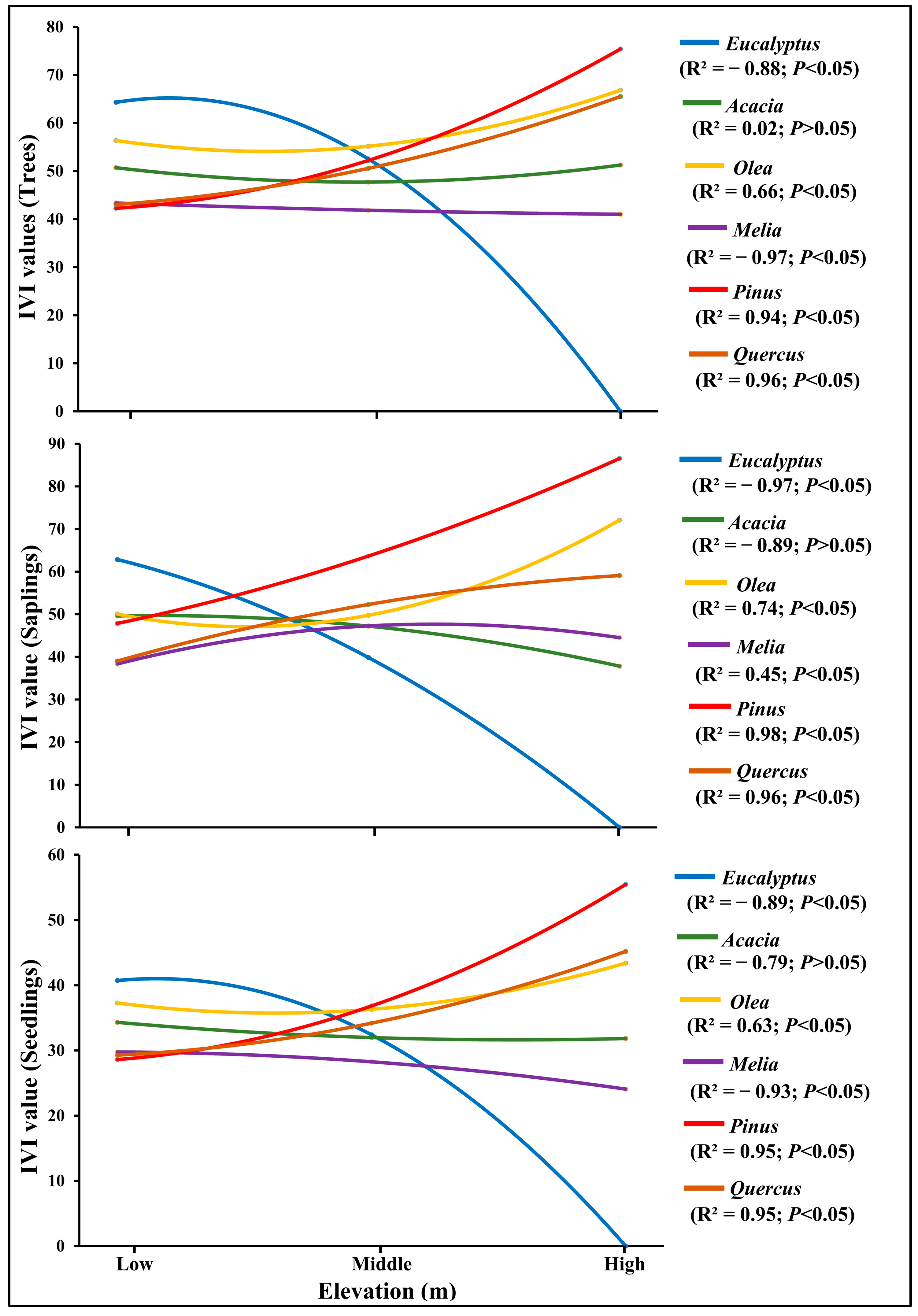
3.3. Association between IVI Value with Elevation Gradient and DBH Classes

The Association of the Important Value Index (IVI) of different tree species with elevation gradient and DBH classes was significant [F(4,53) = 5.12, p < 0.01]. At low elevation for DBH class I, the dominant species was Eucalyptus camaldulensis with IVI 76.40 for trees, 66.41 for saplings, and 47.81 for seedlings, while the co-dominant species was Olea ferruginea with IVI 60.47 for trees, 50.48 for saplings, and 39.22 for seedlings. For DBH class II, the dominant species was Eucalyptus camaldulensis with IVI 61.02 for trees, 68.99 for saplings, and 39.29 for seedlings, while the co-dominant species was Olea ferruginea with IVI 57.18 for trees, 55.80 for saplings, and 38.05 for seedlings. For DBH class III, Eucalyptus camaldulensis was the dominant species with IVI 55.45 for trees and 35.09 for seedlings, and for saplings (IVI—64.70), Pinus roxburghii was the dominant species. In contrast, the co-dominant species was Olea ferruginea for trees and seedlings and Quercus incana for saplings ‘Table S2, Figure 4’.

At the middle elevation for DBH class I, the dominant species was Eucalyptus camaldulensis for trees (67.98), saplings (52.35), and seedlings (40.22), while the co-dominant species was Olea ferruginea for trees (55.14) & seedlings (36.74), and for saplings (52.29) Melia azedarach. For DBH class II, Olea ferruginea was the dominant species for trees and seedlings (55.14) and (37.65), and Pinus roxburghii for saplings (70.30), while the co-dominant species were Pinus roxburghii for trees (57.31) & seedlings (36.95), and for saplings Olea ferruginea (52.97). For DBH class III, the dominant species was Pinus roxburghii for trees (61), saplings (69.58), and seedlings (41.90), while the co-dominant species was Quercus incana with the IVI 59.79 for trees, 60.02 for saplings, and 40.53 for seedlings ‘Table S2, Figure 4’.

No trees, saplings, or seedlings of E. camaldulensis were present at high elevations for all DBH classes. For DBH class I, the dominant species was O. ferruginea for trees (71.07), saplings (83.41), and seedlings (47.77), while the co-dominant species was P. roxburghii for trees, saplings, and seedlings (64.61, 75.47, and 46.03). For DBH class II, the dominant species was P. roxburghii for trees (74.18), saplings (96.08), and seedlings (57.12), while the co-dominant species were Q. incana for trees (70.67), and seedlings (47.52), and O. ferruginea for saplings (66.17). Pinus roxburghii was the dominant species at E3 for DBH class III with the highest value of IVI—87.39 for trees and 63.29 for seedlings, while the co-dominant species were Quercus incana for trees (68.84) and seedlings (51.61), and for saplings Olea ferruginea (66.65) ‘Table S2, Figure 4’.

In association with elevation gradients for tree IVI, all species were influenced significantly except Acacia modesta (R² = 0.02; p > 0.05), while Pinus roxburghii and Quercus incana were the dominant species that were most influenced positively by elevation (R² = 0.94 and 0.96; p < 0.05). However, Eucalyptus camaldulensis and Melia azedarach were influenced negatively (R² = −0.88 and −0.97; p < 0.05). For saplings and seedlings, Pinus roxburghii and Quercus incana were the species that influenced positively (R² = 0.98 and 0.96; p < 0.05 for saplings, and R² = 0.95 and 0.95; p < 0.05 for seedlings). In comparison, Eucalyptus camaldulensis and Acacia modesta were the most negatively influenced species by elevation (R² = −0.97 and −0.89; p < 0.05 for saplings, and R² = −0.89 and −0.79; p < 0.05 for seedlings) ‘Figure 5’.

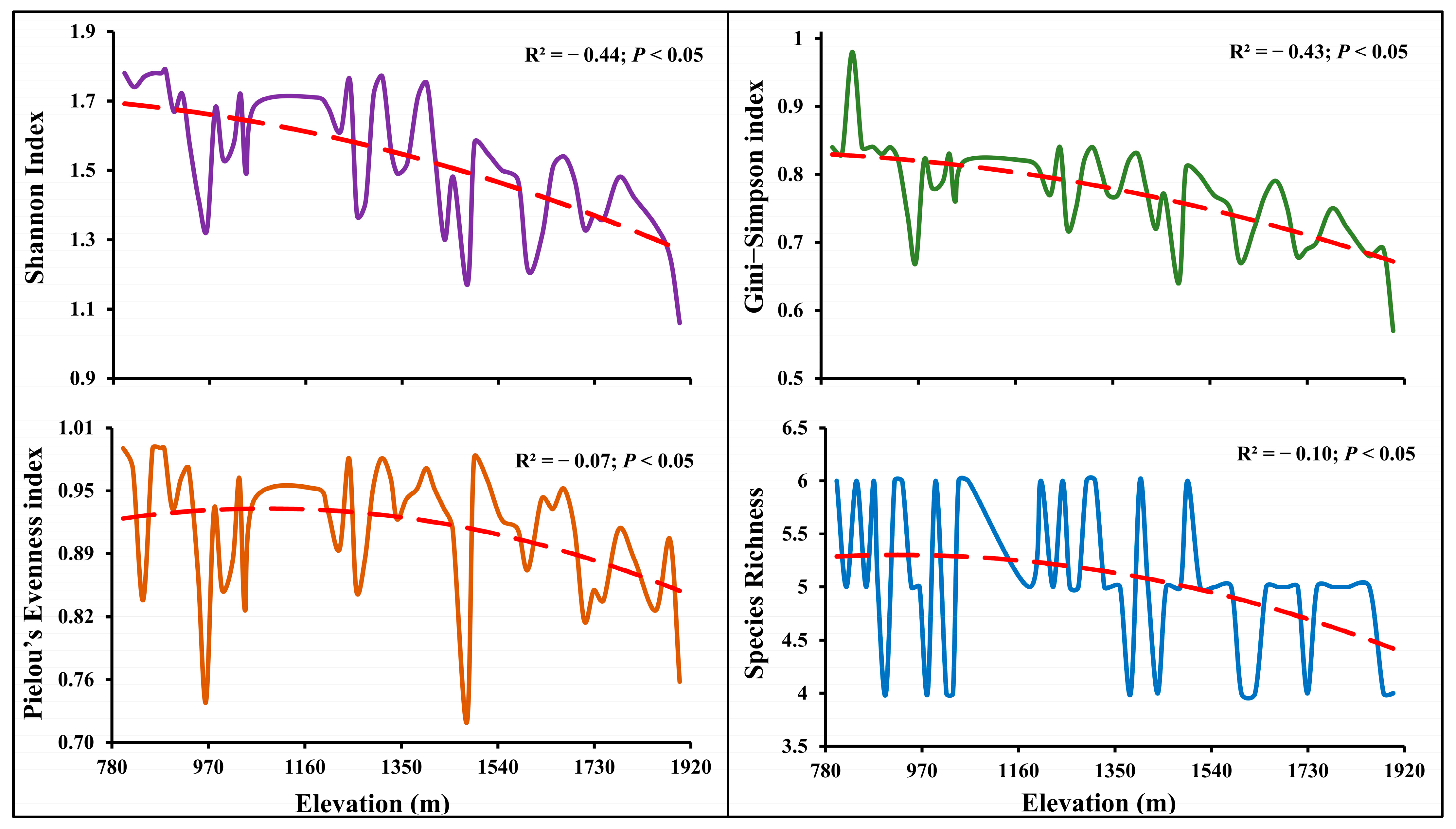
3.4. Association of Species Diversity with Elevation Gradients

According to the analysis of variance (ANOVA), the effect of elevation on species diversity was significant [F(5,305) = 367.24; p < 0.01]. The variability in Shannon and Simpson explained by elevation was significant enough to address their association. Shannon-Weiner Index association with elevation was negatively correlated [R² = −0.44; p < 0.05] ‘Figure 6’ with the highest value (1.64 ± 0.04) at low elevation and lowest value (1.39 ± 0.03) at high elevation for trees and also same pattern for the saplings and seedlings ‘

Table 5. Species diversity indices of trees, saplings, and seedlings concerning elevation gradients. Values are presented as (mean ± SE).

Elevation (m)	Size Class	Shannon-Weiner Index	Gini-Simpson Index	Evenness Index	Species Richness	Abundance
Low	Tree	1.64 ± 0.04	0.81 ± 0.02	0.92 ± 0.02	5.88 ± 0.09	63.47 ± 4.55
	Sapling	1.35 ± 0.1	0.74 ± 0.04	0.84 ± 0.03	5 ± 0.3	57.12 ± 4.9
	Seedling	1.27 ± 0.12	0.76 ± 0.03	0.8 ± 0.06	4.82 ± 0.26	51.88 ± 5.2
Middle	Tree	1.55 ± 0.04	0.78 ± 0.01	0.92 ± 0.02	5.38 ± 0.15	54.88 ± 3.8
	Sapling	1.2 ± 0.1	0.61 ± 0.06	0.69 ± 0.06	4.94 ± 0.2	50.59 ± 3.29
	Seedling	1.07 ± 0.14	0.59 ± 0.06	0.79 ± 0.05	4.59 ± 0.35	48.88 ± 3.42
High	Tree	1.39 ± 0.03	0.72 ± 0.01	0.89 ± 0.01	4.75 ± 0.11	49.41 ± 2.27
	Sapling	1.03 ± 0.12	0.59 ± 0.07	0.68 ± 0.03	4.18 ± 0.29	44.17 ± 2.96
	Seedling	0.98 ± 0.14	0.55 ± 0.06	0.66 ± 0.08	4.06 ± 0.22	44.47 ± 2.57

’. Gini-Simpson Index association with elevation was also correlated negatively [R² = −0.43; p < 0.05] with the highest value (0.81 ± 0.02) at low elevation and lowest value (0.72 ± 0.01) at high elevation for trees, the same pattern was observed for saplings and seedlings. Pileous Species Evenness and Species Richness were also correlated negatively with elevation [R² = −0.07 and −0.10; p < 0.05] ‘Figure 6’. The highest value for species evenness was observed (0.92 ± 0.02) at low elevation and lowest (0.89 ± 0.01), whereas species richness was also recorded as high (5.88 ± 0.09) at low elevation and lowest (4.75 ± 0.11) at high elevation ‘Table 5’. Species Abundance was also reduced significantly [F(1,50) = 6.74; p < 0.05] as the elevation increased. The highest species abundance value (63.47 ± 4.55) was observed at low elevations, which was reduced to (49.41 ± 2.27) at high elevations ‘Table 5’.

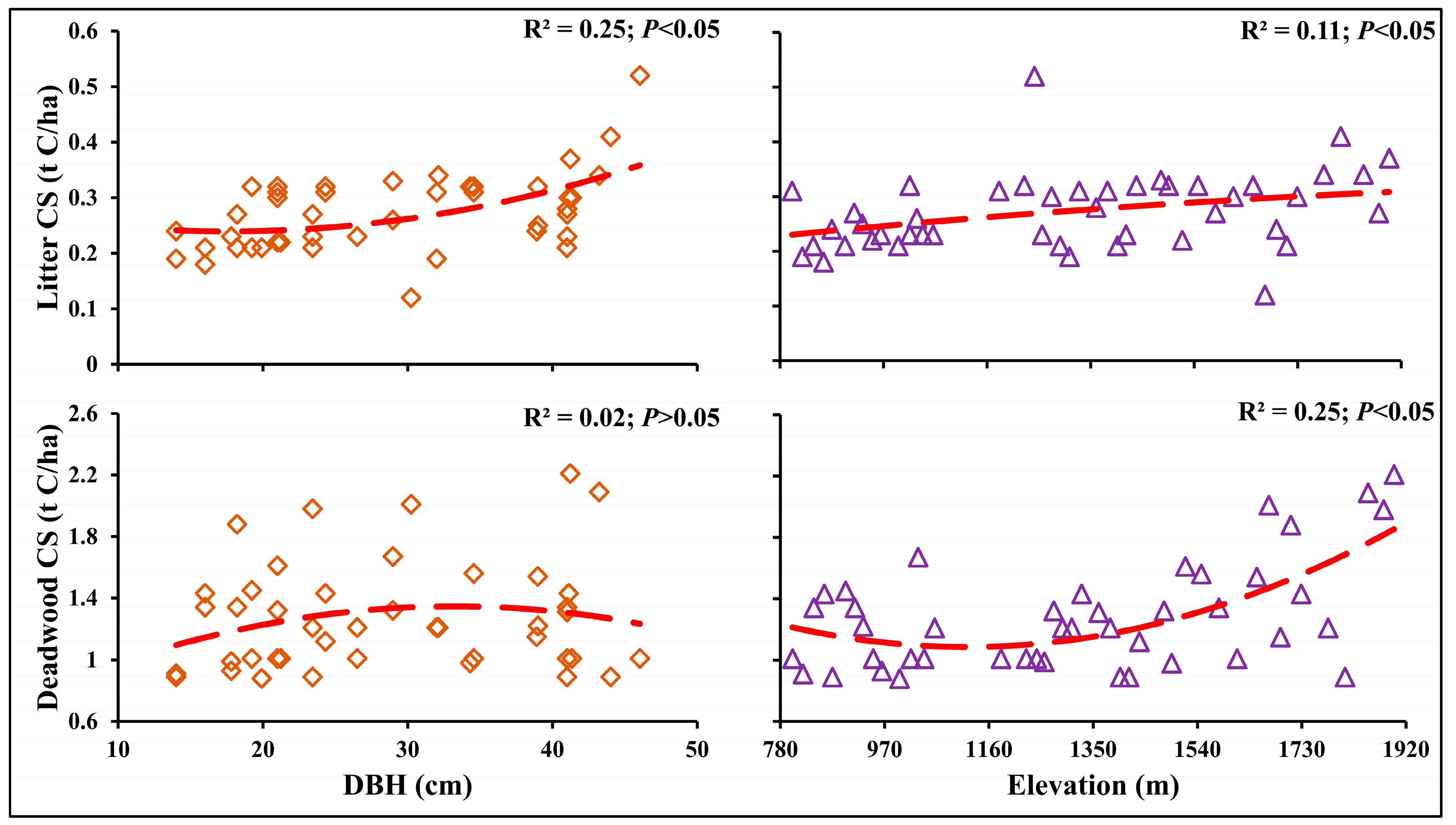
3.5. Association between Litter and Deadwood Carbon with Elevation Gradients

The effect of elevation and DBH on litter biomass and carbon stock was observed to be significant [F(1,44) = 5.84; p > 0.05, and F(1,44) = 14.41; p > 0.05]; Litter biomass ranged between 0.73 ± 0.02 to 1.05 ± 0.04 kg/ha with the highest value for DBH Class-III at E3 and lowest for DBH Class-I at low elevation ‘

Table 6. Litter Biomass (LB), Litter Carbon Stock (LCS), Deadwood Biomass (DWB), and Deadwood Carbon Stock (DWCS), association with elevation gradients and DBH classes. Values are presented as (mean ± SE).

Elevation (m)	DBH Class (cm)	LB (kg/ha)	LCS (t C/ha)	DWB (kg/ha)	DWCS (t C/ha)
Low	I	0.73 ± 0.02	0.23 ± 0.01	3.60 ± 0.06	1.12 ± 0.04
	II	0.76 ± 0.02	0.24 ± 0.01	3.84 ± 0.07	1.19 ± 0.04
	III	0.80 ± 0.02	0.25 ± 0.01	3.99 ± 0.07	1.24 ± 0.4
Middle	I	0.80 ± 0.02	0.25 ± 0.01	3.97 ± 0.08	1.23 ± 0.05
	II	0.90 ± 0.03	0.28 ± 0.01	4.15 ± 0.09	1.29 ± 0.05
	III	0.91 ± 0.02	0.28 ± 0.01	4.20 ± 0.08	1.30 ± 0.06
High	I	0.93 ± 0.03	0.29 ± 0.02	3.81 ± 0.07	1.18 ± 0.06
	II	0.99 ± 0.03	0.31 ± 0.02	4.85 ± 0.09	1.50 ± 0.07
	III	1.05 ± 0.04	0.33 ± 0.02	4.46 ± 0.08	1.38 ± 0.07

’. Whereas deadwood biomass and carbon stock were observed to be affected significantly by elevation [F(1,44) = 14.77; p < 0.05], while non-significant was observed for DBH (p > 0.05). Deadwood biomass ranged between 3.60 ± 0.06 to 4.85 ± 0.09 kg/ha, with the highest value for DBH Class-II at high elevation and lowest for DBH Class-I at low elevation ‘Table 6’. Litter Carbon Stock was significantly correlated positively with DBH [R² = 0.25; p < 0.05] and elevation [R² = 0.11; p < 0.05]. Deadwood correlation with the elevation was significantly positive [R² = 0.25; p < 0.05], while the correlation with DBH was non-significant [R² = 0.02; p > 0.05] ‘Figure 7’.

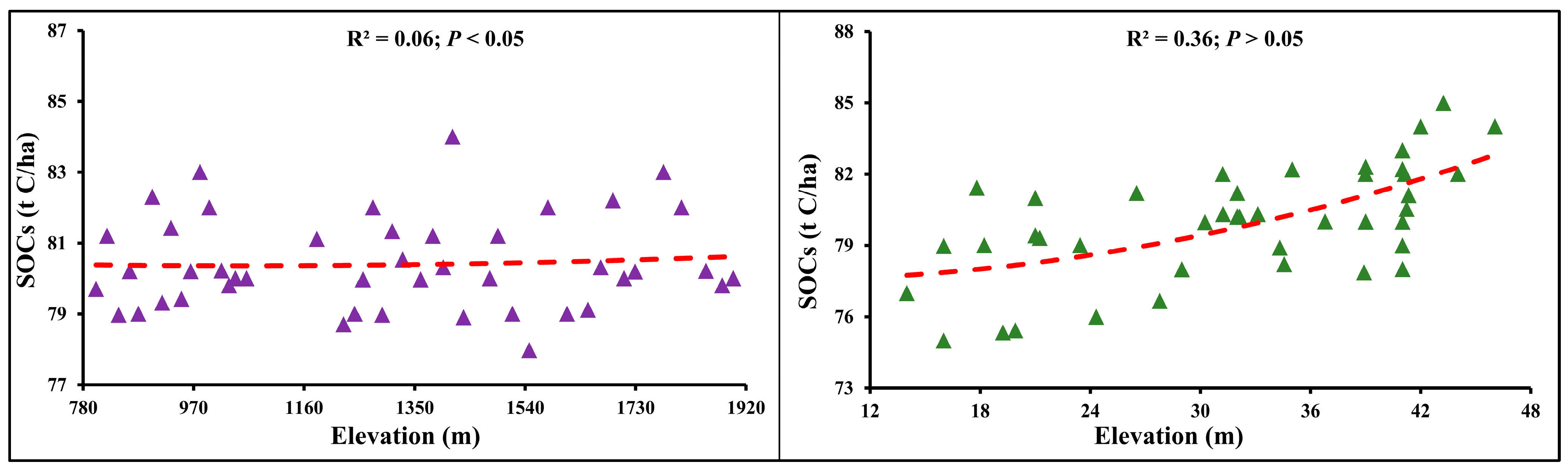
3.6. SOC Association with Elevation Gradients and DBH Classes

The effect of elevation on SOC was observed to be non-significant [F(1,44) = 2.74; p > 0.05]; however, DBH Classes significantly influence the SOC [F(1,44) = 27.13; p < 0.05]. Bulk density ranged between 1.38 ± 0.03 to 1.90 ± 0.06 g/cm³ for all three DBH classes at each location ‘

Table 7. Bulk Density (BD), Soil organic carbon (SOC) contents, and Soil Organic Carbon Stock (SOCS) association with elevation gradients and DBH classes. Values are presented as (mean ± SE).

Elevation (m)	DBH Classes	BD (g/cm3)	SOC (kg/ha)	SOCS (t C/ha)
Low	I	1.38 ± 0.03	42.64 ± 0.17 c	78.53 ± 0.31 b
	II	1.56 ± 0.04	43.39 ± 0.17 b	80.54 ± 0.32 a
	III	1.73 ± 0.05	44.30 ± 0.18 a	81.25 ± 0.33 a
Middle	I	1.39 ± 0.03	44.55 ± 0.18 a	80.01 ± 0.33 b
	II	1.65 ± 0.05	44.75 ± 0.18 a	81.67 ± 0.34 a
	III	1.71 ± 0.05	45.21 ± 0.19 a	82.09 ± 0.34 a
High	I	1.63 ± 0.04	44.68 ± 0.19 b	81.05 ± 0.33 b
	II	1.72 ± 0.05	44.84 ± 0.19 b	81.17 ± 0.34 b
	III	1.90 ± 0.06	45.58 ± 0.20 a	82.15 ± 0.35 a

Letter a, b, c indicating the mean difference between groups (Tukey posthoc test).

’. SOCS was significantly correlated positively with DBH [R² = 0.37; p < 0.05], with the highest (82.15 ± 0.35 t C/ha) for DBH class-III at high elevation and the lowest was (78.53 ± 0.31 t C/ha) for DBH class-I at low elevation. However, no significant association between elevation and SOCS was observed [R² = −0.06; p > 0.05] ‘Figure 8’.

3.7. Carbon Pool Association with Elevation Gradients and DBH Classes

According to ANOVA, all the carbon pool variables were significantly associated with elevation gradients (p < 0.05) except sapling (SCS) and soil (SOCS) carbon stock (p > 0.05), while with DBH classes, all the variables were associated significantly (p < 0.05) except saplings (SCS), and deadwood (DCS) (p > 0.05) ‘Table S3’. According to the Multi-Linear Regression model (MLR), all carbon pool variables were negatively correlated with elevation (p < 0.05) with the highest correlation value for above ground, below ground, and total carbon stock [R² = −0.72, −0.72, and −0.73]; however, litter and deadwood carbon stock increased with the increase in elevation gradient. In contrast, sapling and soil carbon stocks had no significant influence (p > 0.05). However, carbon pool association with DBH classes was significantly correlated negatively for all variables (p < 0.05) except litter and soil carbon stocks, which have a positive association with DBH (R² = 0.19 and 0.39). The highest correlation value was observed for above and below-ground carbon stock [R² = −0.50]; however, DBH classes did not influence deadwood carbon stock (p > 0.05) ‘

Table 8. Association of carbon pools with elevation gradients and diameter classes.

Parameters	Carbon Pools	Adj. R2	p-Value
Elevation	AGCS	−0.72 **	0.00
	BGCS	−0.72 **	0.00
	SCS	−0.28	0.06
	LCS	0.18 **	0.00
	DCS	0.23 **	0.00
	SOCS	0.06	0.16
	TCS	−0.73 **	0.00
DBH	AGCS	−0.50 **	0.00
	BGCS	−0.50 **	0.00
	SCS	−0.36 *	0.02
	LCS	0.19 *	0.04
	DCS	0.05	0.76
	SOCS	0.39 **	0.00
	TCS	−0.45 **	0.00

** Correlation is significant at the 0.01 level (2-tailed). * Correlation is significant at the 0.05 level (2-tailed). AGBCS = Above ground biomass carbon stock, BGBCS = Below ground biomass carbon stock, LCS = litter carbon stock, DWCS = Deadwood carbon stock, SOCS = Soil Organic carbon stock, TCS = Total carbon stock.

’. The highest values of above-ground, below-ground, and sapling carbon stock pools were observed at low elevation, which gradually decreased to the minimum at high elevation, while litter, deadwood, and soil carbon pools were minimum at low elevation and maximum at high elevation. However, for DBH classes, only litter and soil carbon pool values increased with the increase in the DBH, while the rest gradually decreased with the increase in DBH ‘Figure 9’. The highest carbon stock (845.89 t C/ha) was calculated at low elevations, which decreased to (516.27 t C/ha) at high elevations ‘Table S4, Figure 9’.

4. Discussion

4.1. Elevation and DBH Classes Impact Tree Growth Parameters, Litter, and Deadwood Accumulation

In this study, we examined subtropical broadleaved and conifer forest growth parameters, species composition and diversity, and calculation of carbon pool. We discovered that stem density was highest for DBH class-I at low elevation and lowest for DBH class-III at high elevation. We also discovered that as tree diameter increases, stem density per hectare significantly decreases (R² = −0.33), indicating that increasing tree diameter causes stem density to decrease [34]. Furthermore, the relationship between elevation gradients and density was also negatively linked (R² = −0.41), which was consistent with the findings of Yohannes et al. [40] that density was reported to be lower at higher altitudes than it was at lower elevations. Tree height and diameter were positively correlated, while elevation showed no strong correlation. The diameter and elevation of a stand showed a negative correlation with its density. These results are consistent with those of Khan et al. [32], who found that the tree height increased significantly with increasing diameter. However, low stand density at higher elevations compared to lower could be because of certain reasons, i.e., (1) cold temperatures may hinder the growth and development of some tree species at higher elevations, resulting in lower stand densities [59]; (2) variations in precipitation rate at higher elevation gradients cause a shift in stand density [60]; (3) and species composition changes can alter competition for resources in different elevation zones, which in turn affects stand density [61]. In this study, we found out that the basal area and tree volume association with the elevation gradients were negatively correlated, whereas with DBH, both had positive associations. Amir et al. [36] and Khan et al. [32] have reported that stands with high DBH values have high basal area and tree volume compared to the smaller DBH stands. In three diameter classes of six distinct forest tree species—five broadleaved and one conifer—the current study discovered a considerable variance in the biomass of live trees. The carbon content of living tree biomass increases steadily in all tree species as the diameter advances with age.

Furthermore, as elevation rises, this pattern continues to decrease. These findings are consistent with those of Cao et al. [62] and Li et al. [63], who found that stand age and diameter had a substantial impact on the carbon content of tree biomass. The distribution and richness of understory vegetation can be influenced by trees [64]. The microenvironment, degradation of the humus layer, soil moisture, and forest management practices are all impacted by forest stand structure, and factors like tree age and density significantly affect understory flora and litter/deadwood layer [32]. The carbon content of each forest biome depends on several factors, including the pace of decomposition, the species of tree, the maintenance methods used, and the fertility of the litter [65]. We revealed that dead wood and litter accumulation in the ground layer biomass increased significantly as elevation gradients increased. At high elevations, the biomass carbon supply from deadwood and litter was at its highest value ‘Table 4, Figure 4’.

Along with DBH, there was also an increase in the litter layer. The reason for this might be that the forest floor at higher elevations is covered in more deadwood, litter, and leaves than at lower elevations, meaning that trees with larger DBHs—that is, larger tree heights and canopies—enhance natural leaf pruning and shredding. Nevertheless, there was no discernible correlation between DBH classes and deadwood ‘Table 4, Figure 4’. This result correlates with Ming et al. [66], who found that increased diameter eventually increased litter production. Furthermore, compared to lesser DBH, the stand with bigger DBH had a greater layer of deadwood and litter [32,36].

4.2. Species Dominance and Diversity along Elevation Gradients

Out of six tree species, Eucalyptus camaldulensis was the dominant species at low elevation for all DBH classes, while Olea ferruginea was the co-dominant species. At the middle elevation for aDBH class-I, E. camaldulensis was the dominant species, with O. ferriginea as the co-dominant species; but for DBH class-II, the dominant species was O. ferruginea with co-dominant species as Pinus roxburghii, and for DBH class-III, dominant species was P. roxburghii with co-dominant species Quercus incana. At high elevation for DBH class-I, O. ferruginea was the dominant species with P. roxburghii as a co-dominant species, whereas for DBH class-II & III, the dominant species were P. roxburghii and co-dominant species were Q. incana. However, E. camaldulensis was completely absent at higher elevations; one of the reasons is that E. camaldulensis is not the native species of this region; most of it was planted by local communities to support their daily wood needs; also, a lot of E. camaldulensis and other species were planted in KPK after 2018 and onward aiming ‘Billion Tree Tsunami Project’ [67]. Plantations were mainly done in lower regions, bridging the gaps and increasing the forest density. E. camaldulensis is a fast-growing species with wide adaptability [68], so it was chosen for afforestation and reforestation. On the other hand, at E3, P. roxburghii was the dominant species as at such elevations in Pakistan, P. roxburghii thrives well alongside Q. incana as its climax species [32,34,35,36].

Species richness is often believed to decrease with elevation [25]. However, a comprehensive analysis of the literature by Rahbek [69] revealed that almost half of the studies had a species richness peak at mid-altitude [70,71]. On the other hand, the concentration of soil organic carbon (SOC) tends to rise with elevation [72]. These elements highlight how crucial elevation is in determining the dynamics of carbon and biological processes in highland ecosystems.

Along the elevational gradient, there was a shifting tendency in the densities of E. camaldulensis, O. ferruginea, P. roxburghii, Q. incana, Acacia modesta, and Melia azedarach. Climate (temperature and moisture) and edaphic conditions may cause the variance in seedling, sapling, and tree densities [73]. Similar variations in the density of seedlings, saplings, and trees throughout the altitudinal gradient in Nepal and Southern Ethiopia have been reported by Rana et al. [73] and Tesfeye et al. [74]. At lower elevation (E1), the density of trees, saplings, and seedlings of all tree species—aside from P. roxburghii and Q. incana—was high ‘Table 5, Figure 5’. High elevations may have had a negative impact on the survival of seedlings and saplings of all species, particularly Eucalyptus, due to the large basal area and density ‘Figure 5’. P. roxburghii and Q. incana seedling and sapling densities were greater at high elevations, while the densities of E. camaldulensis and O. ferruginea saplings and seedlings were higher at low elevations ‘Figure 5’. Wardle [75] states that seedling density frequently escalates as altitude drops. A greater proportion of seedlings survive in gap areas, and improved germination capability is one of the reasons for more seedlings in gaps [76].

According to Shannon and Simpson diversity indices, species diversity was highest at low elevations, which gradually reduced with increasing elevation; also, species richness was recorded higher at low elevations than at high elevations ‘Table 6, Figure 7’. The decline in species diversity at higher altitudes compared to lower altitudes supports the theory that fewer species are at higher altitudes [77]. It is most likely the result of ecophysiological limitations, including a shorter growth season, colder temperatures, and lower energy [78,79]. Native grasses vary in height [80], while in lowland montane forests, ferns, herbs, and shrubs are among the nonwoody species reported to grow with elevation [81]. This tendency, however, is reversed in forests found in hilly areas, where increased species diversity is found at lower elevations [82]. The mid-domain effect, a prevalent ecological pattern where richness increases along environmental gradients to a point and then begins to decrease, may be responsible for these differing effects of elevation and species diversity within different ecosystems [77,83]. Several theories explain this impact, including geography, temperature, precipitation, and competition [22], and up to some extend climate change too is responsible for that [84].

4.3. Elevation and DBH as a Driver of SOC and Carbon Pool

It is highly challenging to compare SOC with forest biomass [85] since SOC can be impacted by various factors, including environment, standing age, tree species, forest structure, and the chemical and physical characteristics of the soil [86]. In the top soil layer (0–30 cm), soil organic carbon was recorded higher for the DBH class III compared to the other two classes. It might be linked to the growth of SOC by breaking down the root system and debris that first reached the topsoil close to the ground [87]. Elevation causes the temperature to decrease more quickly than litter development, reduces the breakdown of organic matter, and improves SOC [88]. There was a positive correlation between soil carbon and different diameter classes, as soil carbon values tend to increase with increasing diameter. However, no significant effect of elevation gradients on SOC was recorded (p > 0.05) ‘Figure 8’. Khan et al. [32] and Amir et al. [36] reported that the topsoil layer of the forest has a higher percentage of SOC, which tends to increase with diameter.

Every carbon pool outcome in the current investigation differed among DBH classes and elevation gradients. Elevation does not affect sapling or soil carbon stocks and has a significant difference and inverse correlation with all carbon pools except litter and deadwood carbon stock. In contrast, DBH classes have a significant difference and inverse correlation with all carbon pools except for litter, deadwood, and soil carbon stock. This finding aligns with Gairola et al. [89], who discovered a negative relationship between tree biomass and elevation. Likewise, research has indicated in previous studies that biomass carbon storage reduces with altitude [90]. The current study’s findings are similar to those of Simegn and Soromessa [91] in that the lower elevation (E1) stores the most AG and BG carbon storage and the most depleted carbon storage at higher altitudes. Based on the average finding, it is reasonable to conclude that carbon escalates as elevation descends. The rationale for the current study may be that lower elevations have a greater productive stem density than higher elevations. Even though several studies have shown that soil and litter biomass carbon increases with elevation [92,93]. The current study found that whereas soil carbon stock did not significantly change with elevation, the mean carbon content of litter biomass did. The general pattern of the forest’s total mean carbon store is comparable to that of AG and BG carbon. It might be because the carbon pool from above-ground biomass is primarily responsible for the total carbon density.

5. Conclusions

This study has demonstrated that elevation and DBH classes impact forest growth and carbon stock. Each carbon pool exhibits variation throughout the elevational gradient for various DBH classes. Furthermore, elevation and DBH classes are major factors in the above-ground and below-ground carbon pool accounts. This study further showed that forests’ structure, composition, variety, and regeneration varied along elevation gradients, with higher values of these attributes found in lower and medium altitudes. All DBH classes experienced a decline in stem density as elevation ascended. The stem density of forests at lower and higher elevations also differ significantly.

On the other hand, Eucalyptus camaldulensis was the dominating species at lower elevations, with Olea ferruginea as the co-dominant species and Pinus roxburghii as the dominant species, with Quercus incana as a co-dominant species in higher elevation forests, where regeneration was more significant. Elevation gradients and DBH classes played a significant role in forest carbon stock, composition, diversity, and carbon pools in our study. To monitor forest vigor and causes of damage, future studies evaluating the fine-scale elevation gradients of Pinus roxburghii, Quercus incana, Olea ferruginea, and Eucalyptus camaldulenis in this forest will be beneficial. In the end, this study offers important guidelines for doing research of a similar nature in areas of the world that are yet unknown but have great potential for their forests.

References

1. Aryal, S.; Shrestha, S.; Maraseni, T.; Wagle, P.; Gaire, N. Carbon stock and its relationships with tree diversity and density in community forests in Nepal. Int. For. Rev. 2018, 20, 263–273. [Google Scholar] [CrossRef]
2. Pan, Y.; Birdsey, R.A.; Fang, J.; Houghton, R.; Kauppi, P.E.; Kurz, W.A.; Phillips, O.L.; Shvidenko, A.; Lewis, S.L.; Canadell, J.G.; et al. A Large and Persistent Carbon Sink in the World’s Forests. Science 2011, 333, 988–993. [Google Scholar] [CrossRef]
3. FAO. Global Forest Resources Assessment 2020: Main Report; FAO: Rome, Italy, 2020. [Google Scholar]
4. Aryal, S.; Bhattarai, D.R.; Devkota, R.P. Comparison of Carbon Stocks Between Mixed and Pine-Dominated Forest Stands Within the Gwalinidaha Community Forest in Lalitpur District, Nepal. Small-Scale For. 2013, 12, 659–666. [Google Scholar] [CrossRef]
5. Pandey, S.S.; Maraseni, T.N.; Cockfield, G. Carbon stock dynamics in different vegetation dominated community forests under REDD+: A case from Nepal. For. Ecol. Manag. 2014, 327, 40–47. [Google Scholar] [CrossRef]
6. Neupane, P.; Gauli, A.; Maraseni, T.; Kübler, D.; Mundhenk, P.; Dang, M.; Köhl, M. A segregated assessment of total carbon stocks by the mode of origin and ecological functions of forests: Implication on restoration potential. Int. For. Rev. 2017, 19, 120–147. [Google Scholar] [CrossRef]
7. Thuille, A.; Schulze, E. Carbon dynamics in successional and afforested spruce stands in Thuringia and the Alps. Glob. Chang. Biol. 2006, 12, 325–342. [Google Scholar] [CrossRef]
8. Sharma, C.M.; Baduni, N.P.; Gairola, S.; Ghildiyal, S.K.; Suyal, S. Tree diversity and carbon stocks of some major forest types of Garhwal Himalaya, India. For. Ecol. Manag. 2010, 260, 2170–2179. [Google Scholar] [CrossRef]
9. Dawud, S.M.; Raulund-Rasmussen, K.; Domisch, T.; Finér, L.; Jaroszewicz, B.; Vesterdal, L. Is Tree Species Diversity or Species Identity the More Important Driver of Soil Carbon Stocks, C/N Ratio, and pH? Ecosystems 2016, 19, 645–660. [Google Scholar] [CrossRef]
10. Rajput, B.S.; Bhardwaj, D.R.; Pala, N.A. Factors influencing biomass and carbon storage potential of different land use systems along an elevational gradient in temperate northwestern Himalaya. Agrofor. Syst. 2017, 91, 479–486. [Google Scholar] [CrossRef]
11. Andivia, E.; Rolo, V.; Jonard, M.; Formánek, P.; Ponette, Q. Tree species identity mediates mechanisms of top soil carbon sequestration in a Norway spruce and European beech mixed forest. Ann. For. Sci. 2016, 73, 437–447. [Google Scholar] [CrossRef]
12. Sun, X.; Tang, Z.; Ryan, M.G.; You, Y.; Sun, O.J. Changes in soil organic carbon contents and fractionations of forests along a climatic gradient in China. For. Ecosyst. 2019, 6, 1. [Google Scholar] [CrossRef]
13. Reyna-Bowen, L.; Lasota, J.; Vera-Montenegro, L.; Vera-Montenegro, B.; Błońska, E. Distribution and Factors Influencing Organic Carbon Stock in Mountain Soils in Babia Góra National Park, Poland. Appl. Sci. 2019, 9, 3070. [Google Scholar] [CrossRef]
14. Gamfeldt, L.; Snall, T.; Bagchi, R.; Jonsson, M.; Gustafsson, L.; Kjellander, P.; Ruiz-Jaen, M.C.; Froberg, M.; Stendahl, J.; Philipson, C.D.; et al. Higher levels of multiple ecosystem services are found in forests with more tree species. Nat. Commun. 2013, 4, 1340. [Google Scholar] [CrossRef] [PubMed]
15. Hounkpatin, O.K.; de Hipt, F.O.; Bossa, A.Y.; Welp, G.; Amelung, W. Soil organic carbon stocks and their determining factors in the Dano catchment (Southwest Burkina Faso). CATENA 2018, 166, 298–309. [Google Scholar] [CrossRef]
16. Zinn, Y.L.; Andrade, A.B.; Araujo, M.A.; Lal, R. Soil organic carbon retention more affected by altitude than texture in a forested mountain range in Brazil. Soil Res. 2018, 56, 284–295. [Google Scholar] [CrossRef]
17. Zhu, M.; Feng, Q.; Qin, Y.; Cao, J.; Li, H.; Zhao, Y. Soil organic carbon as functions of slope aspects and soil depths in a semiarid alpine region of Northwest China. CATENA 2017, 152, 94–102. [Google Scholar] [CrossRef]
18. Hofhansl, F.; Chacón-Madrigal, E.; Fuchslueger, L.; Jenking, D.; Morera-Beita, A.; Plutzar, C.; Silla, F.; Andersen, K.M.; Buchs, D.M.; Dullinger, S.; et al. Climatic and edaphic controls over tropical forest diversity and vegetation carbon storage. Sci. Rep. 2020, 10, 5066. [Google Scholar] [CrossRef] [PubMed]
19. Takeuchi, T.; Kobayashi, T.; Nashimoto, M. Altitudinal differences in bark stripping by sika deer in the subalpine coniferous forest of Mt. Fuji. For. Ecol. Manag. 2011, 261, 2089–2095. [Google Scholar] [CrossRef]
20. Swetnam, T.L.; Brooks, P.D.; Barnard, H.R.; Harpold, A.A.; Gallo, E.L. Topographically driven differences in energy and water constrain climatic control on forest carbon sequestration. Ecosphere 2017, 8, e01797. [Google Scholar] [CrossRef]
21. Zhao, C.; Zhu, Y.; Meng, J. Effects of Plot Design on Estimating Tree Species Richness and Species Diversity. Forests 2022, 13, 2003. [Google Scholar] [CrossRef]
22. Dieler, J.; Uhl, E.; Biber, P.; Müller, J.; Rötzer, T.; Pretzsch, H. Effect of forest stand management on species composition, structural diversity, and productivity in the temperate zone of Europe. Eur. J. For. Res. 2017, 136, 739–766. [Google Scholar] [CrossRef]
23. Silaeva, T.; Andreychev, A.; Kiyaykina, O.; Balčiauskas, L. Taxonomic and ecological composition of forest stands inhabited by forest dormouse Dryomys nitedula (Rodentia: Gliridae) in the Middle Volga. Biologia 2021, 76, 14751482. [Google Scholar] [CrossRef]
24. Wang, J.; Hu, A.; Meng, F.; Zhao, W.; Yang, Y.; Soininen, J.; Shen, J.; Zhou, J. Embracing mountain microbiome and ecosystem functions under global change. New Phytol. 2022, 234, 1987–2002. [Google Scholar] [CrossRef] [PubMed]
25. Whittaker, R.J.; Willis, K.J.; Field, R. Scale and species richness: Towards a general, hierarchical theory of species diversity. J. Biogeogr. 2001, 28, 453–470. [Google Scholar] [CrossRef]
26. Lomolino, M.V. Elevation gradients of species-density: Historical and prospective views. Glob. Ecol. Biogeogr. 2001, 10, 3–13. [Google Scholar] [CrossRef]
27. Tashi, S.; Singh, B.; Keitel, C.; Adams, M. Soil carbon and nitrogen stocks in forests along an altitudinal gradient in the eastern Himalayas and a meta-analysis of global data. Glob. Chang. Biol. 2016, 22, 2255–2268. [Google Scholar] [CrossRef] [PubMed]
28. Bukhari, B.S.S.; Haider, A.; Laeeq, M.T. Land Cover Atlas of Pakistan; Pakistan Forest Institute: Peshawar, Pakistan, 2012; p. 140. [Google Scholar]
29. MOCC. Readiness Preparation Proposal (RPP) for Pakistan; Ministry of Climate Change, Government of Pakistan Islamabad: Islamabad, Pakistan, 2013. [Google Scholar]
30. Hayat, U.; Abbas, A.; Shi, J. Public Attitudes towards Forest Pest Damage Cost and Future Control Extent: A Case Study from Two Cities of Pakistan. Forests 2024, 15, 544. [Google Scholar] [CrossRef]
31. Hayat, U.; Akram, M.; Kour, S.; Arif, T.; Shi, J. Pest Risk Assessment of Aeolesthes sarta (Coleoptera: Cerambycidae) in Pakistan under Climate Change Scenario. Forests 2023, 14, 253. [Google Scholar] [CrossRef]
32. Khan, I.; Hayat, U.; Mujahid, A.; Majid, A.; Chaudhary, A.; Badshah, M.; Huang, J. Evaluation of growing stock, biomass and soil carbons and their association with a diameter: A case study from a planted chir pine (pinus roxburghii) forest. Appl. Ecol. Environ. Res. 2021, 19, 1457–1472. [Google Scholar] [CrossRef]
33. Ali, A.; Ashraf, M.I.; Gulzar, S.; Akmal, M. Estimation of forest carbon stocks in temperate and subtropical mountain systems of Pakistan: Implications for REDD+ and climate change mitigation. Environ. Monit. Assess. 2020, 192, 198. [Google Scholar] [CrossRef]
34. Nizami, S.M. The inventory of the carbon stocks in sub tropical forests of Pakistan for reporting under Kyoto Protocol. J. For. Res. 2012, 23, 377–384. [Google Scholar] [CrossRef]
35. Ahmad, A.; Nizami, S.M. Carbon stocks of different land uses in the Kumrat valley, Hindu Kush Region of Pakistan. J. For. Res. 2015, 26, 57–64. [Google Scholar] [CrossRef]
36. Amir, M.; Liu, X.; Ahmad, A.; Saeed, S.; Mannan, A.; Muneer, M.A. Patterns of Biomass and Carbon Allocation across Chronosequence of Chir Pine (Pinus roxburghii) Forest in Pakistan: Inventory-Based Estimate. Adv. Meteorol. 2018, 2018, 3095891. [Google Scholar] [CrossRef]
37. Hayat, U.; Khan, I.; Roman, M. A response of tropical tree Terminalia arjuna (Ar-jun)[Combretaceae-Myrtales] seeds and seedlings towards the presowing seed treatment in forest nursery of Sargodha, Paki-stan. Int. J. Biosci. 2020, 16, 495–505. [Google Scholar] [CrossRef]
38. PMD. Pakistan Metrological Department. 2023. Available online: https://www.pmd.gov.pk/en/ (accessed on 29 September 2023).
39. Bhishma, P.S.; Shiva, S.P.; Ajay, P.; Eak, B.R.; Sanjeeb, B.; Tibendra, R.B.; Shambhu, C.; Rijan, T. Forest Carbon Stock Measurement: Guidelines for Measuring Carbon Stocks in Community-Managed Forests; Funded by Norwegian Agency for Development Cooperation (NORAD); Asia Network for Sustainable Agriculture and Bioresources (ANSAB) Publishing: Kathmandu, Nepal, 2020; pp. 17–43. [Google Scholar]
40. Yohannes, H.; Soromessa, T.; Argaw, M. Carbon stock analysis along slope and slope aspect gradient in Gedo Forest: Im-plications for climate change mitigation. J. Earth Sci. Clim. Change 2015, 6, 6–11. [Google Scholar] [CrossRef]
41. Pearson, T.R.; Walker, S.; Brown, S. Sourcebook for Land-Use, Land-Use Change and Forestry Projects; Winrock International and the Bio-carbon fund of the World Bank: Arlington, TX, USA, 2005; pp. 19–35. Available online: https://winrock.org/wp-content/uploads/2016/03/Winrock-BioCarbon_Fund_Sourcebook-compressed.pdf (accessed on 10 January 2024).
42. IPCC [Intergovernmental Panel on Climate Change]. Good Practice Guidance for Land Use, Land-Use Change and Forestry; Intergovernmental Panel on Climate Change: Geneva, Switzerland, 2003; p. 590. [Google Scholar]
43. Ali, A.; Ashraf, M.I.; Gulzar, S.; Akmal, M. Development of an Allometric Model for Biomass Estimation of Pinus roxburghii, Growing in Subtropical Pine Forests of Khyber Pakhtunkhwa, Pakistan. Sarhad J. Agric. 2020, 36, 236–244. [Google Scholar] [CrossRef]
44. Ali, A. Biomass and Carbon Tables for Major Tree Species of Khyber Pakhtunkhwa; Pakistan Forest Institute: Peshawar, Pakistan, 2020. [Google Scholar]
45. Miah, D.; Islam, K.N.; Kabir, H.; Koike, M. Allometric models for estimating aboveground biomass of selected homestead tree species in the plain land Narsingdi district of Bangladesh. Trees For. People 2020, 2, 100035. [Google Scholar] [CrossRef]
46. Khan, I.A.; Khan, W.R.; Ali, A.; Nazre, M. Assessment of Above-Ground Biomass in Pakistan Forest Ecosystem’s Carbon Pool: A Review. Forests 2021, 12, 586. [Google Scholar] [CrossRef]
47. Hairiah, K.; Sitompul, S.M.; Van Noordwijk, M.; Palm, C. Methods for Sampling Carbon Stocks above and Below Ground; ICRAF: Bogor, Indonesia, 2001; pp. 1–23. Available online: https://apps.worldagroforestry.org/downloads/Publications/PDFS/LN01114.PDF (accessed on 10 January 2024).
48. Morisada, K.; Ono, K.; Kanomata, H. Organic carbon stock in forest soils in Japan. Geoderma 2003, 119, 21–32. [Google Scholar] [CrossRef]
49. Hartley, J.; Marchant, J. Methods of Determining the Moisture Content of Wood; Technical Paper No. 41; Research Division, State Forests of New South Wales: Sydney, Austria, 1995; p. 61. [Google Scholar]
50. Agus, F.; Hairiah, K.; Mulyani, A. Measuring Carbon Stock in Peat Soils: Practical Guidelines; World Agroforestry Centre (ICRAF) Southeast Asia Regional Program, Indonesian Centre for Agricultural Land Resources Research and Development: Bogor, Indonesia, 2011; 60p, Available online: https://citeseerx.ist.psu.edu/document?repid=rep1&type=pdf&doi=e639e6e20348e8db564cf12b832b7f5286b84db3 (accessed on 10 January 2024).
51. Rahman, M.H.; Holmes, A.W.; Deurer, M.; Saunders, S.J.; Mowat, A.; Clothier, B.E. Comparison of three methods to estimate organic carbon in allophanic soils in New Zealand. In Proceedings of the 24th Annual FLRC Workshop, Auckland, New Zealand, 8–10 February 2011; Massey University: Auckland, New Zealand, 2011; p. 4. [Google Scholar]
52. Curtis, J.T.; McIntosh, R.P. An Upland Forest Continuum in the Prairie-Forest Border Region of Wisconsin. Ecology 1951, 32, 476–496. [Google Scholar] [CrossRef]
53. Chapagain, U.; Chapagain, B.P.; Nepal, S.; Manthey, M. Impact of Disturbances on Species Diversity and Regeneration of Nepalese Sal (Shorea robusta) Forests Managed under Different Management Regimes. Earth 2021, 2, 826–844. [Google Scholar] [CrossRef]
54. Gracia, M.; Montané, F.; Piqué, J.; Retana, J. Overstory structure and topographic gradients determining diversity and abundance of understory shrub species in temperate forests in central Pyrenees (NE Spain). For. Ecol. Manag. 2007, 242, 391–397. [Google Scholar] [CrossRef]
55. Yeom, D.-J.; Kim, J.H. Comparative evaluation of species diversity indices in the natural deciduous forest of Mt. Jeombong. For. Sci. Technol. 2011, 7, 68–74. [Google Scholar] [CrossRef]
56. Shannon, C.E.; Wiener, W. The Mathematical Theory of Communities; University of Illinois Press: Urbana, IL, USA, 1963; p. 117. [Google Scholar]
57. Pielou, E.C. The measurement of diversity in different types of biological collections. J. Theor. Biol. 1966, 13, 131–144. [Google Scholar] [CrossRef]
58. Simpson, E.H. Measurement of diversity. Nature 1949, 163, 668. [Google Scholar] [CrossRef]
59. Körner, C. The use of ‘altitude’in ecological research. Trends Ecol. Evol. 2007, 22, 569–574. [Google Scholar] [CrossRef] [PubMed]
60. Lloyd, A.H.; Fastie, C.L. Spatial and Temporal Variability in the Growth and Climate Response of Treeline Trees in Alaska. Clim. Change 2002, 52, 481–509. [Google Scholar] [CrossRef]
61. Liang, M.; Liu, X.; Etienne, R.S.; Wang, Y.; Staehelin, C. Does facilitation and competition of two shrubs with different eleva-tion distribution patterns change with environmental stress? Plant Soil 2016, 408, 393–404. [Google Scholar]
62. Cao, J.; Wang, X.; Tian, Y.; Wen, Z.; Zha, T. Pattern of carbon allocation across three different stages of stand development of a Chinese pine (Pinus tabulaeformis) forest. Ecol. Res. 2012, 27, 883–892. [Google Scholar] [CrossRef]
63. Li, C.; Zha, T.; Liu, J.; Jia, X. Carbon and nitrogen distribution across a chronosequence of secondary lacebark pine in China. For. Chron. 2013, 89, 192–198. [Google Scholar] [CrossRef]
64. Svenning, J.-C.; Skov, F. Mesoscale distribution of understorey plants in temperate forest (Kalø, Denmark): The importance of environment and dispersal. Plant Ecol. 2002, 160, 169–185. [Google Scholar] [CrossRef]
65. Kang, B.; Liu, S.; Zhang, G.; Chang, J.; Wen, Y.; Ma, J.; Hao, W. Carbon accumulation and distribution in Pinus massoniana and Cunninghamia lanceolata mixed forest ecosystem in Daqingshan, Guangxi, China. Acta Ecol. Sin. 2006, 26, 1320–1327. [Google Scholar] [CrossRef]
66. Ming, A.; Jia, H.; Zhao, J.; Tao, Y.; Li, Y. Above- and Below-Ground Carbon Stocks in an Indigenous Tree (Mytilaria laosensis) Plantation Chronosequence in Subtropical China. PLoS ONE 2014, 9, e109730. [Google Scholar] [CrossRef] [PubMed]
67. MOCC. In Ministry of Climate Change and Environmental Coordination, Government of Pakistan; 2023. Available online: https://www.mocc.gov.pk/ProjectDetail/M2QzOWJmMjUtZTU3MC00NmFkLWE4YmMtZDFhMmRlOGU2NGRh (accessed on 10 January 2024).
68. Lindenmayer, D.; Hobbs, R. Fauna conservation in Australian plantation forests—A review. Biol. Conserv. 2004, 119, 151–168. [Google Scholar] [CrossRef]
69. Vetaas, O.R.; Grytnes, J. Distribution of vascular plant species richness and endemic richness along the Himalayan elevation gradient in Nepal. Glob. Ecol. Biogeogr. 2002, 11, 291–301. [Google Scholar] [CrossRef]
70. Rahbek, C. The elevational gradient of species richness: A uniform pattern? Ecography 1995, 18, 200–205. Available online: https://www.jstor.org/stable/3682769 (accessed on 10 January 2024). [CrossRef]
71. Rickart, E.A. Elevational diversity gradients, biogeography and the structure of montane mammal communities in the intermountain region of North America. Glob. Ecol. Biogeogr. 2001, 10, 77–100. [Google Scholar] [CrossRef]
72. Sánchez-Cordero, V. Elevation gradients of diversity for rodents and bats in Oaxaca, Mexico. Glob. Ecol. Biogeogr. 2001, 10, 63–76. [Google Scholar] [CrossRef]
73. Rana, P.; Koirala, M.; Bhuju, D.R.; Boonchird, C. Population structure of Rhododendron campanulatum D. Don and asso-ciated tree species along the elevational gradient of Manaslu conservation area, Nepal. J. Inst. Sci. Technol. 2016, 21, 95–102. [Google Scholar] [CrossRef]
74. Tesfaye, G.; Teketay, D.; Fetene, M.; Beck, E. Regeneration of seven indigenous tree species in a dry Afromontane forest, southern Ethiopia. Flora 2009, 205, 135–143. [Google Scholar] [CrossRef]
75. Wardle, P. An explanation for alpine timberline. N. Z. J. Bot. 1971, 9, 371–402. [Google Scholar] [CrossRef]
76. Qing, L. The effects of gap size and within gap position on the survival and growth of naturally regenerated abies georgei seedlings. Chin. J. Plant Ecol. 2004, 28, 204–209. [Google Scholar] [CrossRef]
77. Colwell, R.K.; Hurtt, G.C. Nonbiological Gradients in Species Richness and a Spurious Rapoport Effect. Am. Nat. 1994, 144, 570–595. [Google Scholar] [CrossRef]
78. Körner, C. Why are there global gradients in species richness? mountains might hold the answer. Trends Ecol. Evol. 2000, 15, 513–514. [Google Scholar] [CrossRef]
79. Brown, J.H. Mammals on mountainsides: Elevational patterns of diversity. Glob. Ecol. Biogeogr. 2001, 10, 101–109. [Google Scholar] [CrossRef]
80. D’antonio, C.M.; Tunison, J.T.; Loh, R.K. Variation in the impact of exotic grasses on native plant composition in relation to fire across an elevation gradient in Hawaii. Austral Ecol. 2000, 25, 507–522. [Google Scholar] [CrossRef]
81. Jimbo, T.; Saulei, S.; Moses, J.; Lawong, B.; Kaina, G.; Kiapranis, R.; Hitofumi, A.; Novotny, V.; Attorre, F.; Testolin, R.; et al. Beyond the Trees: A Comparison of Nonwoody Species, and Their Ecology, in Papua New Guinea Elevational Gradient Forest. Case Stud. Environ. 2023, 7, 1831407. [Google Scholar] [CrossRef]
82. Haq, S.M.; Calixto, E.S.; Rashid, I.; Srivastava, G.; Khuroo, A.A. Tree diversity, distribution and regeneration in major forest types along an extensive elevational gradient in Indian Himalaya: Implications for sustainable forest management. For. Ecol. Manag. 2022, 506, 119968. [Google Scholar] [CrossRef]
83. Colwell, R.; Lees, D.C. The mid-domain effect: Geometric constraints on the geography of species richness. Trends Ecol. Evol. 2000, 15, 70–76. [Google Scholar] [CrossRef]
84. Hayat, U.; Shi, J.; Wu, Z.; Rizwan, M.; Haider, M.S. Which SDM Model, CLIMEX vs. MaxEnt, Best Forecasts Aeolesthes sarta Distribution at a Global Scale under Climate Change Scenarios? Insects 2024, 15, 324. [Google Scholar] [CrossRef]
85. Laganière, J.; Angers, D.A.; Paré, D. Carbon accumulation in agricultural soils after afforestation: A meta-analysis. Glob. Chang. Biol. 2010, 16, 439–453. [Google Scholar] [CrossRef]
86. Mora, J.; Guerra, J.; Armas-Herrera, C.; Arbelo, C.; Rodríguez-Rodríguez, A. Storage and depth distribution of organic carbon in volcanic soils as affected by environmental and pedological factors. CATENA 2014, 123, 163–175. [Google Scholar] [CrossRef]
87. Zhang, H.; Guan, D.; Song, M. Biomass and carbon storage of Eucalyptus and Acacia plantations in the Pearl River Delta, South China. For. Ecol. Manag. 2012, 277, 90–97. [Google Scholar] [CrossRef]
88. Choudhury, B.U.; Fiyaz, A.R.; Mohapatra, K.P.; Ngachan, S. Impact of Land Uses, Agrophysical Variables and Altitudinal Gradient on Soil Organic Carbon Concentration of North-Eastern Himalayan Region of India. Land Degrad. Dev. 2014, 27, 1163–1174. [Google Scholar] [CrossRef]
89. Gairola, S.; Ghildiyal, S.K.; Sharma, C.M.; Suyal, S. Species richness and diversity along an altitudinal gradient in moist temperate forest of Garhwal Himalaya. Am. J. Sci. 2009, 5, 119–128. [Google Scholar]
90. Moser, G.; Hertel, D.; Leuschner, C. Altitudinal Change in LAI and Stand Leaf Biomass in Tropical Montane Forests: A Transect Study in Ecuador and a Pan-Tropical Meta-Analysis. Ecosystems 2007, 10, 924–935. [Google Scholar] [CrossRef]
91. Simegn, T.Y.; Soromessa, T. Carbon Stock Variations Along Altitudinal and Slope Gradient in the Forest Belt of Simen Mountains National Park, Ethiopia. Am. J. Environ. Prot. 2015, 4, 199. [Google Scholar] [CrossRef]
92. Tsui, C.-C.; Chen, Z.-S.; Hsieh, C.-F. Relationships between soil properties and slope position in a lowland rain forest of southern Taiwan. Geoderma 2004, 123, 131–142. [Google Scholar] [CrossRef]
93. Griffiths, R.; Madritch, M.D.; Swanson, A. The effects of topography on forest soil characteristics in the Oregon Cascade Mountains (USA): Implications for the effects of climate change on soil properties. For. Ecol. Manag. 2008, 257, 1–7. [Google Scholar] [CrossRef]
Figure 1. Geographical presentation of the study area illustrating the elevation (m), roughness, hill shade, slope (%), and sampling plots.
Forests 15 01395 g001
Figure 2. (A) Schematic layout of nested square plot design. (B) Schematic nested square plot design with an area of 50 × 50 m for trees, 20 × 20 m area for saplings, 2.82 m for saplings, and 5 × 5 m for seedlings.
Forests 15 01395 g002
Figure 3. Association of tree height and stand density with elevation gradients and diameter classes.
Forests 15 01395 g003
Figure 4. Important value index (IVI) of trees, saplings, and seedlings of six tree species for different DBH classes along the elevational gradient.
Forests 15 01395 g004
Figure 5. Association between elevation gradients and IVI values of trees, saplings, and seedlings of six tree species.
Forests 15 01395 g005
Figure 6. Association between elevation gradients and diversity indices.
Forests 15 01395 g006
Figure 7. Association of Litter and Deadwood carbon stock with elevation (m) and DBH (cm).
Forests 15 01395 g007
Figure 8. Association of SOCS with elevation (m) and DBH (cm).
Forests 15 01395 g008
Figure 9. Influence of elevation gradients and DBH classes on the carbon pool of the study area. AGCS = Above ground carbon stock, BGCS = Below ground carbon stock, SCS = Sapling carbon stock, LCS = Litter carbon stock, DCS = Deadwood carbon stock, SOCS = Soil organic carbon stock, and TCS = Total carbon stock.
Forests 15 01395 g009