Article

Simulating the Long-Term Response of Forest Succession to Climate Change in the Boreal Forest of Northern Ontario, Canada

1
Natural Resources Canada, Canadian Forest Service, Laurentian Forestry Centre, 1055 du P.E.P.S., P.O. Box 10380, Stn. Sainte-Foy, Quebec, QC G1V 4C7, Canada
2
Ontario Forest Research Institute, Ontario Ministry of Natural Resources, 1235 Queen St. E., Sault Ste. Marie, ON P6A 2E5, Canada
*
Author to whom correspondence should be addressed.
Forests 2024, 15(8), 1417; https://doi.org/10.3390/f15081417
Submission received: 20 June 2024 / Revised: 26 July 2024 / Accepted: 8 August 2024 / Published: 13 August 2024
(This article belongs to the Special Issue Forest Growth Modeling in Different Ecological Conditions)

Abstract

:
The effect of climate change on forest dynamics is likely to increase in importance in the forthcoming decades. For this reason, it is essential to predict the extent to which changes in temperature, precipitation, and atmospheric CO2 might affect the development of forest ecosystems and successional pathways. The gap model ZELIG-CFS was used to simulate the potential long-term effects of climate change on species-specific annual change in mean basal area and stand density under two scenarios of representative concentration pathways (RCP), 4.5 and 8.5, for the boreal forest region of Ontario, Canada, where mean temperature, precipitation, and atmospheric CO2 are expected to increase. Forest ecosystems in this boreal region included pure and mixed stands of black spruce (Picea mariana [Mill.] B.S.P.), paper birch (Betula papyrifera Marsh.), balsam fir (Abies balsamea [L.] Mill.), jack pine (Pinus banksiana Lamb.), trembling aspen (Populus tremuloides Michx.), white spruce (Picea glauca [Moench] Voss), northern white cedar (Thuja occidentalis L.), American larch (Larix laricina [Du Roi] K. Koch), and balsam poplar (Populus balsamifera L.). Simulation results under climate change generally predicted a decline in the basal area and stand density for black spruce, balsam fir, jack pine, and white spruce, but an increase for paper birch, trembling aspen, American larch, and balsam poplar. However, the extent of change differed regionally among species. Forest composition is expected to change over the long term. Simulation results indicated that shade-intolerant deciduous and conifer species will increase their dominance over the 100-year time horizon. This transition toward the increasing presence of deciduous forests is likely explained by more favorable temperature conditions for their growth and development.

1. Introduction

The scientific community has recognized for several decades that climate change is a major factor affecting forest ecosystems [1,2]. Most of the processes that regulate tree and stand growth and mortality, demographic processes, and carbon, nutrient, and water cycles will be affected, but many questions still need to be studied extensively to evaluate the extent of the impact of global change [1]. Modeling the effects of climate change on tree and forest productivity and succession has been the focus of many studies for several years. The different studies have relied mostly on the use of dendroclimatic methodology, examination of sample plots or tree historical measurements, and the development of simulation models. Dendrochronological records were used along latitudinal gradients to relate tree ring development to climatic records, e.g., [3,4,5,6,7,8]. Studies based on the analysis of tree or permanent sample plot historical records have the benefit of tracking all facets of forest dynamics, including recruitment, growth, and mortality, which allows the development of statistical relationships with climatic records, e.g., [9,10]. Although rich in detail, both approaches have limitations. For example, they assume that the relationships between tree growth and climatic variables are linear and do not change with time [5]. Also, the use of these relationships beyond the extent of the data used for their development may lead to growth response extrapolation to climatic extremes not experienced by the trees under investigation [5].
The examination of the effects of climate change on forests has also been conducted using empirical and process-based models. For example, Huang et al. [5] combined the use of tree-ring increment data and empirical regression analysis to develop statistical growth models for paper birch (Betula papyrifera Marsh.), black spruce (Picea mariana [Mill.] B.S.P.), jack pine (Pinus banksiana Lamb.), and trembling aspen (Populus tremuloides Michx.) along a large latitudinal gradient in eastern Canada. They assumed that models derived at local scales in the south could be applied in northern locations to predict the potential effects of climate change on forest productivity. However, they recognized that their approach had limitations due to large sources of uncertainty and differences in genetic inheritance and latitudinal variation in the strength of temperature and precipitation effects. Major efforts have been made to develop process-based physiological simulation models to predict the effects of climate change on forest development and carbon cycle, e.g., [11,12,13]. Several models were associated with results or knowledge obtained from experimental conditions, such as free-air CO2 enrichment (FACE) experiments [14]. The general form of this type of model is based on the derivation/use of empirical or theoretical relationships of ecophysiological processes, including photosynthesis and respiration, and biotic and abiotic factors that affect them [14]. Process-based models have the potential to predict the effects of climate change on several ecophysiological processes occurring in forest ecosystems more precisely; however, their complexity requires a strong ability to develop and parameterize them [14]. Also, their development requires several types of ecophysiological data and knowledge that cover the range of variation in ecosystem properties for predicting the effects of climate change on forest ecosystems varying considerably in species composition and soil conditions [15]. Species composition is a key factor, as species differ in their ability to acclimate to changing conditions [16].
Another avenue to simulate the effects of climate change on forest ecosystems includes forest gap models. This type of model is based on the representation of species-specific biotic and abiotic factors, integrating basic ecophysiological understanding of tree and stand growth to simulate forest succession [17]. They do not include detailed representations of ecophysiological processes, such as those in process-based physiological models, but they are more biologically consistent than empirical statistical models [18]. Typical gap models include functions to simulate tree and stand growth and mortality, canopy interactions, and regeneration. They can be easily parameterized using experimental or observational data [19,20,21,22]. The advantages of using gap models to predict the effects of climate change on different forest types have been highlighted several times [23,24,25,26,27,28]. As they have a biological framework, gap models are more easily adaptable for different forest ecosystems compared to empirical models. The degree of confidence in the predictions of empirical growth and yield models, which are derived using statistical methods, is limited by the lower and upper boundaries of the data used for their parameterization [5,29]. For sound calibration, empirical models require large datasets with varied species mixtures on different soil types and climatic conditions to reach the same level of biological consistency as gap models.
Gap models have previously been used to predict the effects of climate change for different types of forest ecosystems, e.g., [30,31]. However, more work is needed to examine different concepts in the modeling of processes involved in successional pathways, including mechanistic approaches, and to evaluate their consistency across forest types and conditions, particularly for mixed uneven-aged boreal forest ecosystems. The objective of the present study was to simulate the change in species composition of boreal forests under two scenarios of climate change in northern Ontario, Canada, using the gap model ZELIG-CFS. It is assumed that no natural or anthropogenic disturbance occurred to isolate the effects of climate change scenarios. Using historical data, an earlier study indicated that ZELIG-CFS realistically predicted the long-term dynamics of mixed uneven-aged boreal forest ecosystems [32]. For the present study, ZELIG-CFS was modified to represent the effects of changes in temperature, precipitation, and atmospheric CO2 on individual tree growth and development. It is hypothesized that the extent of the effects of climate change on the dynamics of forest ecosystems differs among species and occurs gradually. Species intolerant to shade that can live under relatively high degree days are expected to be favored.

2. Materials and Methods

2.1. Overview of the Gap Model ZELIG-CFS

The model used for the present study, ZELIG-CFS, is composed of interactive components to (1) read initialization data, (2) generate annual climatic data, (3) simulate mortality, tree growth rate in diameter at breast height (dbh), and height and regeneration establishment, and (4) report simulation results for each time step at the tree and stand levels. It is a gap model originating from ZELIG [33,34,35] and is similar in concept to JABOWA [36]. ZELIG-CFS is a type of model that is adapted to simulate the growth and succession of mixed-aged forests that contain several species. Also, it integrates ecological characteristics at the species level that influence the form of the relationships that represent how individual tree growth and seedling development are affected by temperature, precipitations, site fertility, and canopy and understory light conditions. Basic ecological characteristics used by ZELIG-CFS for the boreal species are listed in Table 1. Light interception is modeled at different crown levels and canopy scales. Several modifications have improved the computation of competitive interactions at the crown and canopy levels [32,37,38]. In particular, the modeling of the available light growing factor (ALGF) was modified by integrating a sigmoidal function to model cumulative leaf area distribution. This change better represents light interception at different crown levels and takes into account the effect of the shade tolerance class of each species involved in the simulation of forest ecosystems more effectively. Each species belongs to one of five shade tolerance classes that affect the dbh growth rate using logistic relationships. The combination of ALGF and shade tolerance classes influences the crown recession rate, which influences the dbh growth rate. As shown in Table 1, each species also has specific limits of minimum and maximum degree days within which it grows and is categorized by drought and nutrient tolerance classes. Minimum and maximum degree days are used in parabolic relationships to compute the effects of degree days, computed from local temperature data, on the dbh growth rate. Species-specific drought and nutrient tolerance classes are used in hyperbolic and modified inverse functions, respectively, to compute the effects of site fertility and soil moisture on dbh growth rate.
In addition to species-specific basic ecological characteristics and individual dbh data, initialization files to execute ZELIG-CFS include potential regeneration data and stocking. Potential regeneration data include estimates of the number of seedlings per square meter that may develop in each simulation year and stocking. The potential number of seedlings is randomly modified to emulate natural variability and is adjusted to account for light intensity underneath the canopy, soil humidity, fertility level, and temperature [37]. Stocking is an estimate of the proportion of the forest area occupied by the seedlings of a species. ZELIG-CFS was initialized with regeneration and stocking values for each sample plot. These values were based on a literature review, regeneration surveys in northern Ontario and Quebec, and the application of an adjustment factor at the plot level based on estimates related to species-specific density within each plot (Table 2). More details can be found in Larocque and Bell [32]. Other variables included in initialization files consist of soil field capacity and wilting point, annual potential maximum above-ground biomass production, and site-specific mean monthly temperature and precipitation. Monthly climatic data are used to compute annual growing degree days, soil water capacity, and the drought index for each simulation year. ZELIG-CFS performs simulations on an annual time step. Standard deviations associated with monthly temperature and precipitation data are used to randomly compute normally occurring annual variations.
Specific functions were developed in ZELIG-CFS to model forest response to climate change by computing gradual changes in annual monthly mean temperature, precipitation, and atmospheric CO2. For the effect of change in atmospheric CO2 increase, specific functions were developed to compute the percent change in dbh increment rate based on the work by Johnsen and Major [39], Isebrands et al. [40,41], Kubiske et al. [42], Zhang and Dang [43], Cao et al. [44], Marfo and Dang [45], Major et al. [46], and Newaz et al. [47] (Table 3). The percent change effects were assumed to increase linearly from 360 ppm to 720 ppm in CO2 concentration. The relationship developed for black spruce was also used for balsam fir and northern white cedar, as these species have similar ecological characteristics. For the same reason, the relationship developed for trembling aspen was also used for American larch and balsam poplar.
Projected rates of change in temperature, precipitation, and atmospheric CO2 concentration for northern Ontario were obtained from the Climate Atlas of Canada (https://climateatlas.ca, accessed on 25 August 2022). Simulations of forest succession were conducted for two representative concentration pathways (RCP) scenarios, 4.5 and 8.5, representing intermediate and high emission scenarios. Under RCP 4.5, temperature was increased annually by 0.026 °C, precipitation by 0.093%, and atmospheric CO2 by 1.4 ppm. Corresponding changes for RCP 8.5 were 0.049 °C, 0.149%, and 5.14 ppm. The 100-year simulations of forest succession from these two RCP scenarios were compared with a scenario based on unchanged climatic conditions, that is, without change in temperature, precipitation, or atmospheric CO2, to rate the magnitude of the effects of change in climatic conditions (RCP 0). However, for the three scenarios, temperature and precipitation are randomly varied to emulate typical fluctuations that normally occur. These random variations were based on standard deviations calculated from meteorological observations over a 30-year period. Forest succession was simulated for a 100-year time horizon.

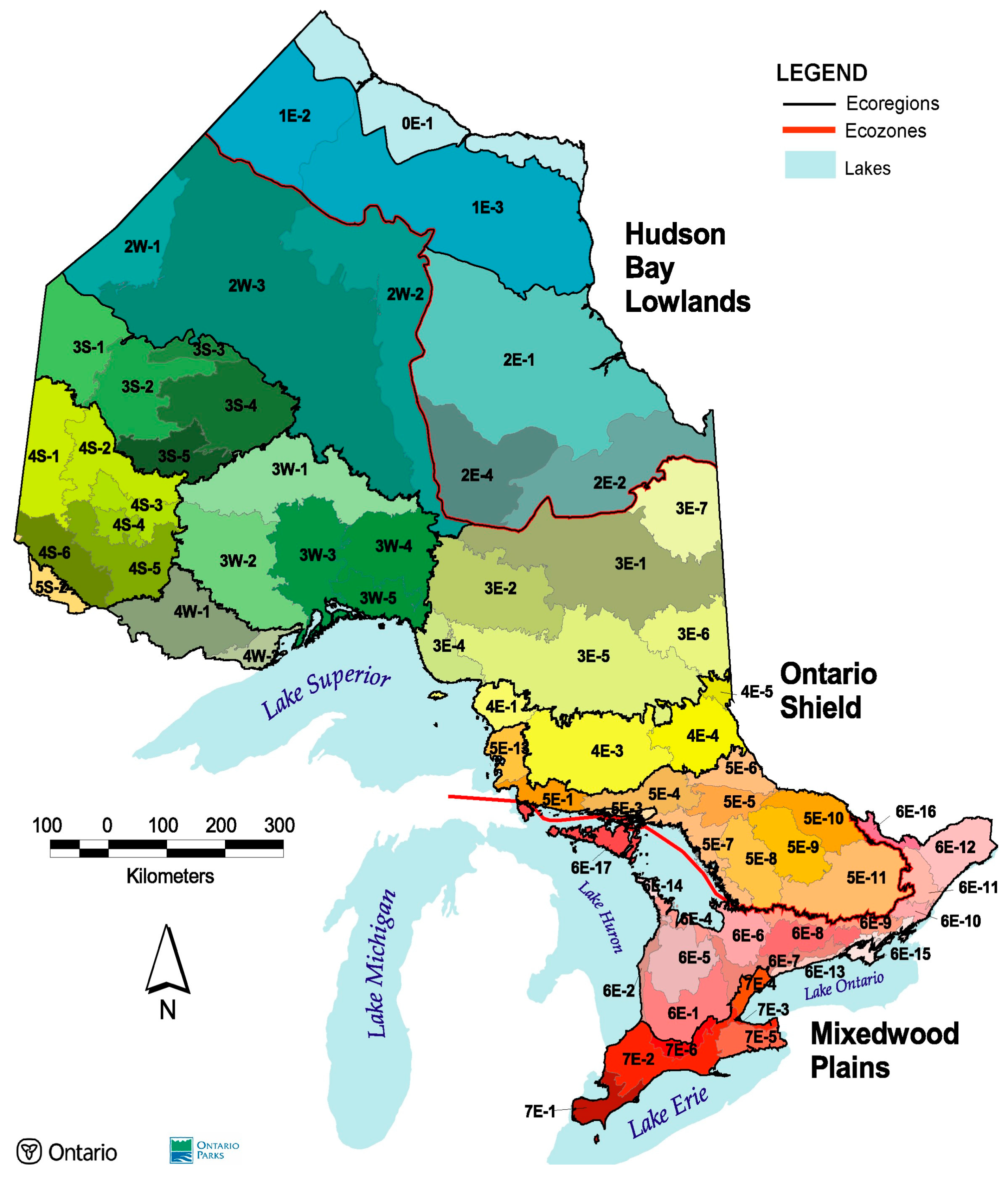
2.2. Study Area and Datasets

This study was conducted in ecoregions 3E and 3W in the boreal forest region of the Ontario Shield Ecozone, Canada [48] (Figure 1). This ecozone, which occupies about 65 million hectares (ha) in northern Ontario, is characterized by a topography that varies considerably. The winter season lasts longer than in southern Ontario, with a cold temperature and high humidity levels. The average daily temperature in January, the middle of the winter season, is about −15 °C and in July, the middle of the summer season, it is 17 °C. Even though ecoregions 3E and 3W are located within the same ecozone, they present differences in ecological properties, which justified a separate compilation of simulation results. Ecoregion 3E is located within the humid mid-boreal ecoclimatic region, with precipitation varying from 652 to 1029 mm year−1. The mean annual temperature range is −0.5 to 2.5 °C and the mean length of the growing season is between 167 and 185 days [49]. Deposits are composed of morainal clays in the northeastern part and mostly ground moraine elsewhere in the ecoregion. The most common soil types in this ecoregion are podzols. Ecoregion 3W belongs to the moist mid-boreal ecoclimatic region, with annual precipitation that varies between 654 and 879 mm, mean annual temperatures between −1.7 to 2.1 °C, and a mean growing season length between 161 to 182 days [49]. Bedrock is characterized by granite, basalt, volcanic rocks, greenstone, siltstone, or shale. Soil types include brunisols or podzols.
Both ecoregions 3E and 3W include the following tree species: black spruce, balsam fir (Abies balsamea [L.] Mill.), white spruce (Picea glauca [Moench] Voss), jack pine, trembling aspen, paper birch, American larch (Larix laricina [Du Roi] K. Koch), northern white cedar (Thuja occidentalis L.), and balsam poplar (Populus balsamifera L.). However, the diversity in species composition varied between ecoregions 3E and 3W (Table 4). The average basal area was higher in ecoregion 3E than 3W for black spruce, American larch, balsam poplar, and trembling aspen. On the other hand, the average basal area was higher for jack pine and paper birch in ecoregion 3W. The mean basal area for balsam fir, white spruce, and northern white cedar was close between both ecoregions. Despite large variations in minimum and maximum basal areas, black spruce, jack pine, and trembling aspen had greater basal areas than the other species in both ecoregions.
ZELIG-CFS was initialized using individual tree data obtained from three datasets developed by three forest companies and maintained by the Ontario Ministry of Natural Resources and Forestry (OMNRF). They were the American Can (148 sample plots), Kimberly Clark (114 sample plots), and Spruce Falls Power and Paper Co. (SFPP) (113 sample plots). For the American Can dataset, 68 and 80 sample plots were in ecoregions 3E and 3W, respectively. All the sample plots of the Kimberly Clark dataset were located in ecoregion 3W and all the sample plots of the SFPP dataset were located in ecoregion 3E. Each tree was measured for dbh in every sample plot. Sample plot size measured from 400 to 4047 m2 and stands varied in age, as young as 5 years and as old as 170 years. Average stand density and dbh varied considerably among trees within species and among species (Table 5). Black spruce had the highest mean stand density in all three datasets but it varied substantially among the sample plots within the three datasets, as low as 12 trees ha−1 and as high as 16,343 trees ha−1. Relative to black spruce, the other species had lower stand density values, but the ranges of variation in stand density were comparable. Mean dbh varied considerably among species: jack pine, trembling aspen, and balsam poplar had relatively high mean dbh values compared to the other tree species in the three datasets. There were also considerable differences in dbh within each species, with values as low as 1.0 and as high as 59.9 cm. The extensive variation in both stand density and dbh values reflects the diversity and mixed nature of the forest ecosystems in the region. Two sets of initialization files were created to execute ZELIG-CFS: one for sample plot data in ecoregion 3E and the second one for sample plot data in ecoregion 3W.

3. Results

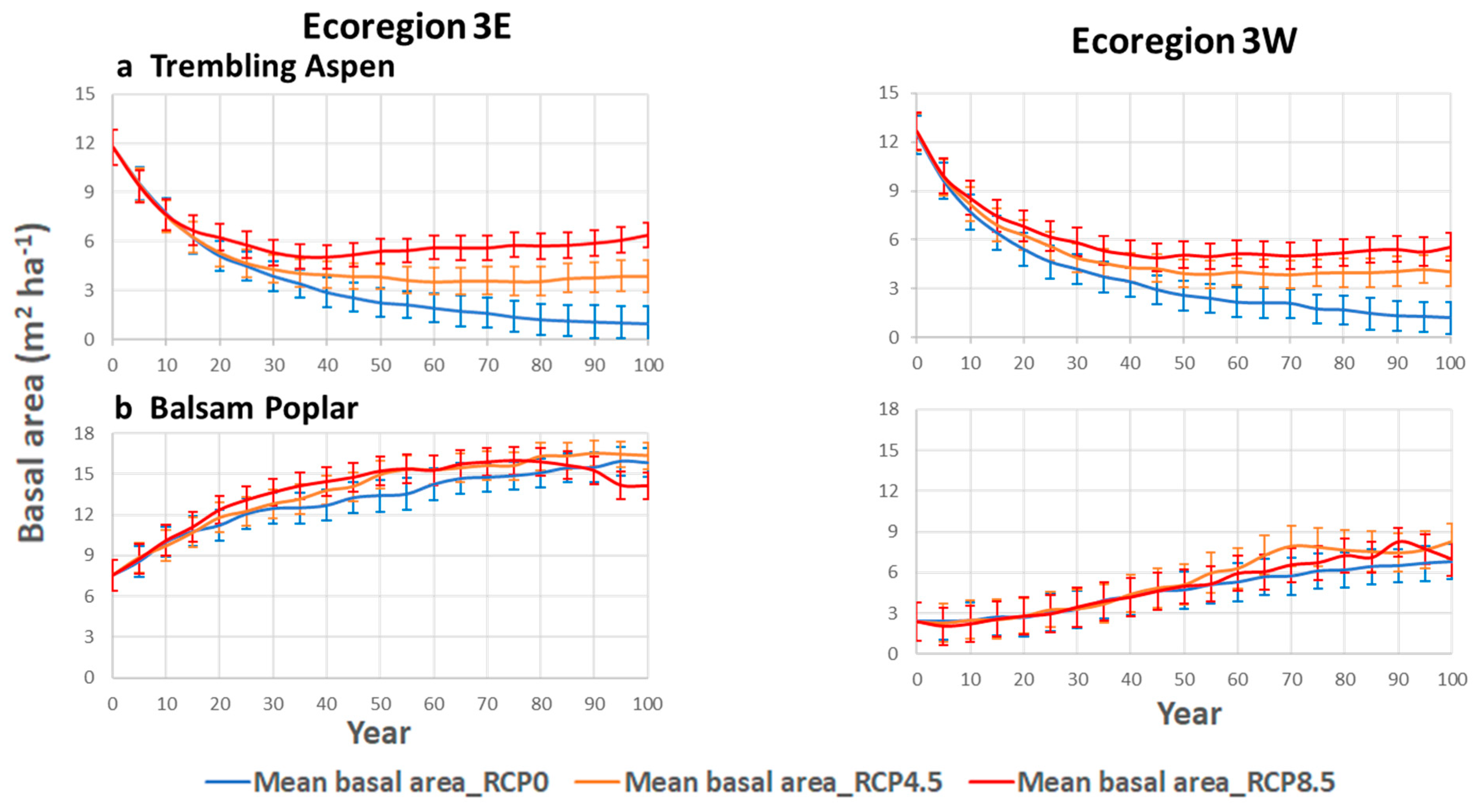
3.1. Mean Basal Area
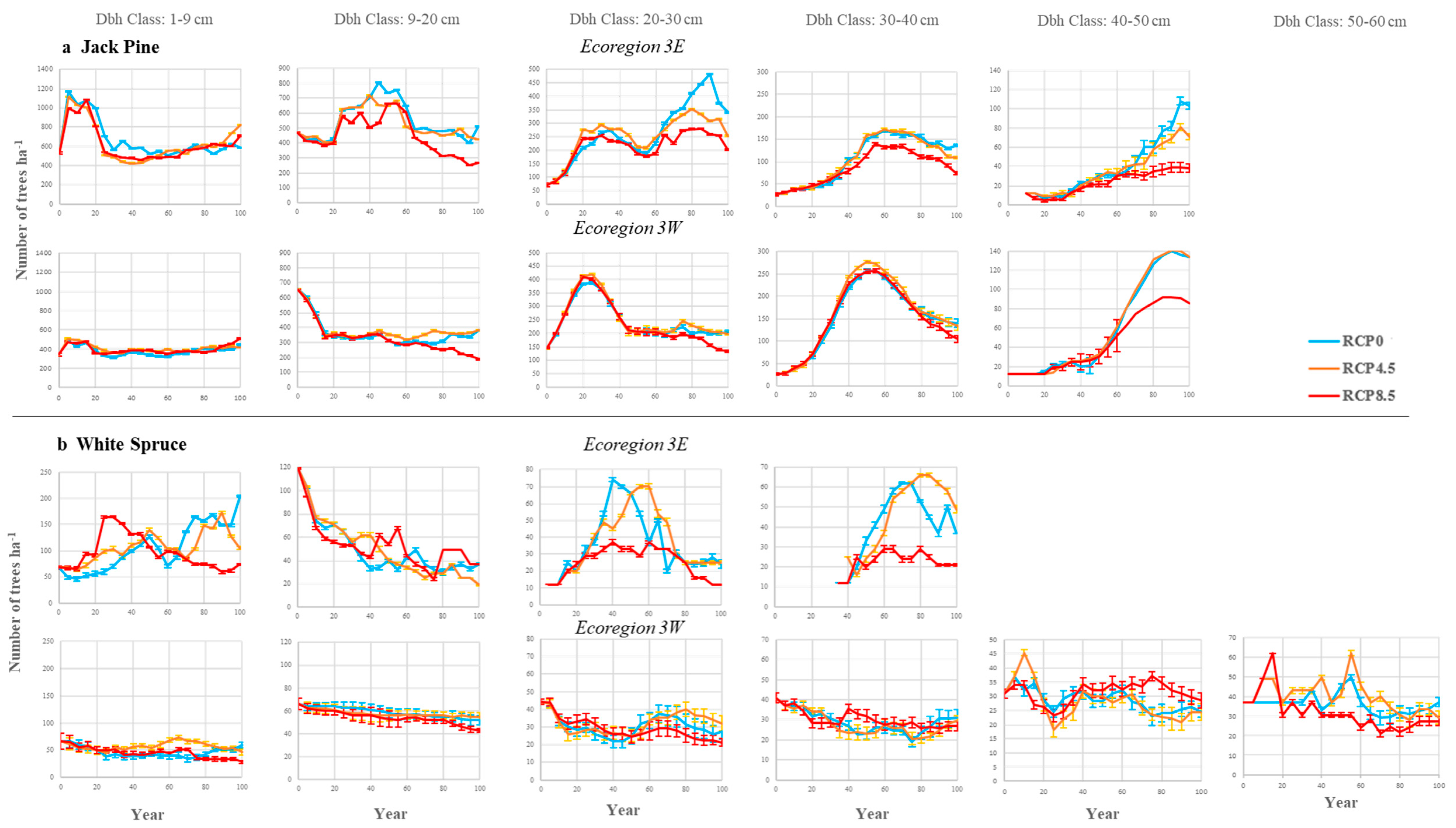
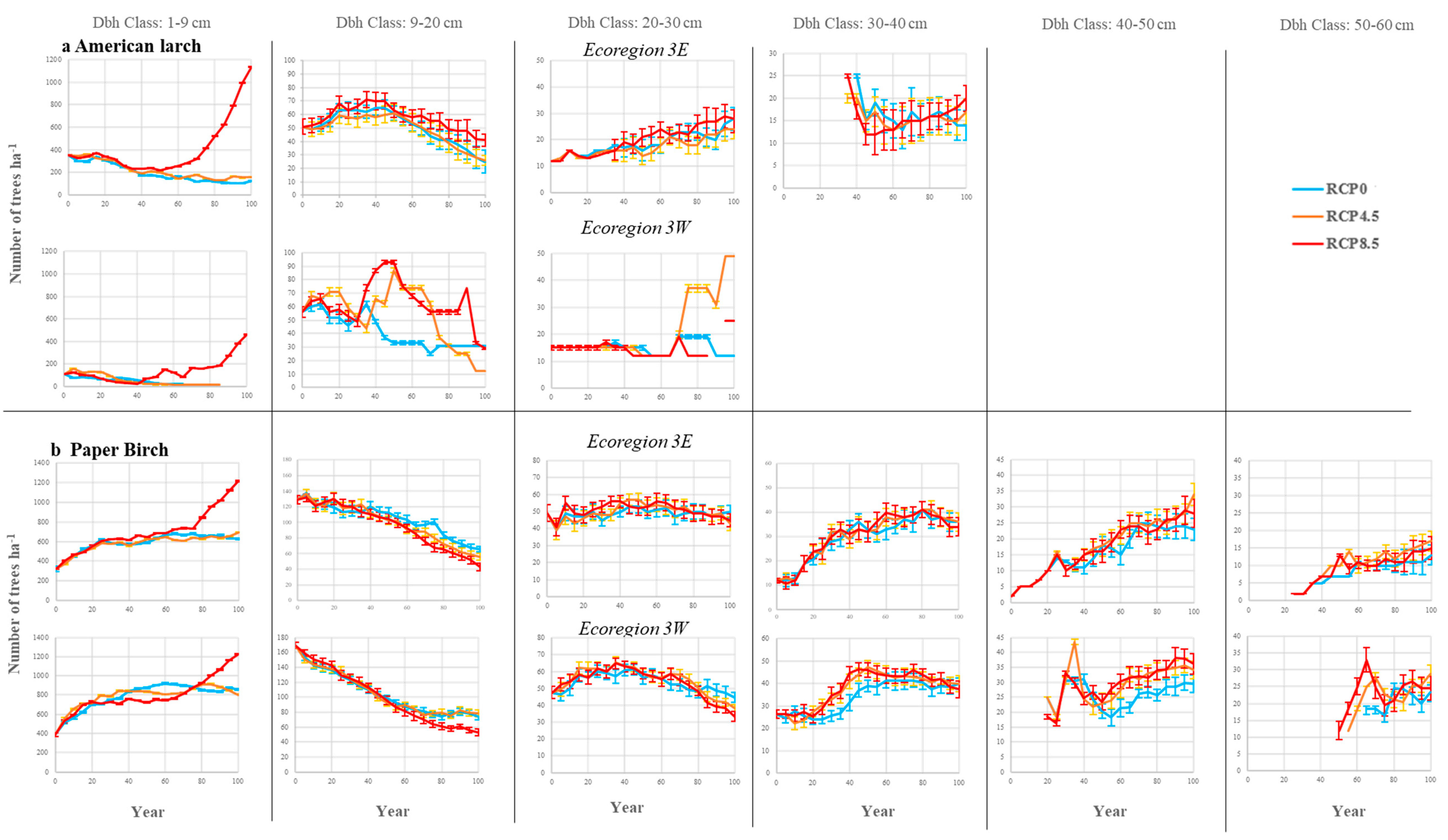
The predicted mean basal area for black spruce differed among the climate change scenarios in the two ecoregions (Figure 2a). Differences among the three scenarios began to appear around year 30 of the simulation in ecoregion 3E and year 40 in ecoregion 3W. Under current climatic conditions (RCP 0), the simulated mean basal area increased in both ecoregions. For the scenario RCP 4.5, the mean basal area reached a maximum around simulation year 70 in ecoregion 3E and year 85 in ecoregion 3W and then very slightly declined. Under scenario RCP 8.5, the mean basal area reached a maximum at year 30 in ecoregion 3E and year 45 in ecoregion 3W and then decreased substantially thereafter. However, by the end of the simulation, the mean basal area reached a slightly lower value in ecoregion 3E than in ecoregion 3W.
For balsam fir, differences in the mean basal area among the three scenarios appeared around years 40 and 24 of the simulations in ecoregions 3E and 3W, respectively (Figure 2b). There was a gradual increase under RCP 0 and this increase was more noticeable in ecoregion 3W than 3E. Under RCP 4.5, the mean basal area also increased in both ecoregions but at a lower pace than RCP 0. The mean basal area under RCP 8.5 increased until years 50 and 65 of the simulations in ecoregions 3E and 3W, respectively, and then gradually declined. Jack pine showed some differences in the pattern of change between both ecoregions (Figure 2c). In ecoregion 3E, relatively similar values in mean basal area were obtained under RCP 0 and 4.5 throughout the 100-year simulation, while the mean basal area under RCP 4.5 was slightly higher in ecoregion 3W. For both ecoregions, the mean basal area under RCP 8.5 increased until about year 30 of the simulations, remained stable until simulation year 70, and then declined. The decline relative to RCP 0 was more pronounced in ecoregion 3E and occurred earlier in the simulations.
The temporal pattern of change in the mean basal area for white spruce differed between both ecoregions (Figure 3a). Higher mean basal area values were reached in ecoregion 3E than 3W under RCP 0 and 4.5, which were remarkably close throughout the simulations. The mean basal area under RCP 8.5 increased until simulation year 65 and then decreased to reach a value close to simulation year 0. On the other hand, in ecoregion 3W, the mean basal area was higher under RCP 4.5 and 8.5 relative to RCP 0 and differences between RCP 4.5 and 8.5 were less pronounced than in ecoregion 3E. Also, differences between both scenarios appeared later in ecoregion 3W than 3E.
The mean basal area for American larch increased gradually over the 100-year simulation in ecoregion 3E (Figure 3b). While the increase in mean basal area under RCP 4.5 occurred more slowly than that under RCP 0, it increased at a faster rate under RCP 8.5. Results for ecoregion 3W diverged from those for ecoregion 3E. The mean basal area under RCP 0 and 4.5 increased until simulation year 100. Under RCP 8.5, the increase in mean basal area was less pronounced. The large overlaps between the error bars suggest that American larch was not affected by climate change scenarios. The mean basal area for paper birch increased throughout the course of simulations in both ecoregions (Figure 3c). The simulation results for this species under both RCP 4.5 and 8.5 were remarkably close until the simulated years 70 to 80. Differences between RCP 0 and both RCP 4.5 and 8.5 appeared early in the simulations but were less pronounced than those for other species.
Trembling aspen showed a decrease in mean basal area for all three scenarios in both ecoregions (Figure 4a). While it stabilized around simulation year 40 in RCP 4.5 and 8.5, the mean basal area gradually decreased until simulation year 100 under RCP 0. The mean basal area for balsam poplar was higher in ecoregion 3E than 3W (Figure 4b). Under all three RCP scenarios in both ecoregions, the mean basal area gradually increased until simulation year 100, except under RCP 8.5, which slightly declined by years 80 and 90 in ecoregions 3E and 3W, respectively. Differences in mean values between RCP 0 and RCP 4.5 and 8.5 appeared around year 20 in ecoregion 3E and year 50 in ecoregion 3W, but differences were relatively less pronounced than for most of the other species.

3.2. Stand Density

Simulation results for stand density were grouped into different dbh classes (Figure 5, Figure 6, Figure 7 and Figure 8). For most species, some dbh classes showed differences among climate change scenarios and both ecoregions, while there was no difference for other dbh classes.
For black spruce in ecoregion 3E, differences among RCP scenarios were observed for simulated stand density within the dbh classes 1–9 cm, 20–30 cm, and 30–40 cm (Figure 5a). While RCP 0 and 4.5 did not differ much for the dbh class 1–9 cm, simulated stand density began to decrease under RPC 8.5 relative to RCP 0 around year 40. The simulated stand density did not differ substantially among the three scenarios within the 9–20 cm dbh class and was characterized by a decreasing pattern. For the dbh classes 20–30 cm and 30–40 cm, stand density increased under the three RCP scenarios but the increase was more pronounced under RCP 0 and 4.5. Relative to RCP 0 and 4.5, stand density became much lower under RCP 8.5. For the ecoregion 3W, simulated stand density within the 1–9 cm dbh class did not show differences for the first 70 years and then stand density for RCP 8.5 decreased considerably. Like the results for ecoregion 3E, simulated stand density did not differ among the RCPs and showed a decreasing pattern over time. Changes for simulated stand density for dbh classes 20–30 cm and 30–40 cm were like those within the ecoregion 3E.
The mean stand density for balsam fir within the 1–9 cm dbh class increased until around year 60 and then stabilized thereafter in both ecoregions (Figure 5b). The values for the three RCP scenarios were remarkably close for all simulation years. The effects of RCP 4.5 and 8.5 were more important for the 9–20 cm class. Relative to RCP 0, stand density decreased in RCP 4.5 and 8.5 starting at year 70 in ecoregion 3E and years 40 and 60 in ecoregion 3W, respectively. Stand density within the 20–30 cm class decreased over the simulation period. For both ecoregions, mean stand density among the RCP scenarios did not differ appreciably in both ecoregions, except for RCP 8.5 in ecoregion 3E. Stand density was low within the dbh class 30–40 cm in both ecoregions. Relative to RCP 0, higher values were obtained under RCP 4.5 and 8.5 for several years within the 30–40 cm class for ecoregion 3E but differences among them were not pronounced. For ecoregion 3W, the results were discontinuous. In particular, stand density within the 30–40 cm dbh class appeared much later in the simulations and there was an increase in RCP 8.5.
For jack pine, the effects of RCP 4.5 and 8.5 relative to RCP 0 were not important within the 1–9 cm dbh class for both ecoregions and within the 30–40 cm dbh class within ecoregion 3W (Figure 6a). For both ecoregions, stand density increased in the first 20 years of simulation within the 1–9 cm dbh class and was then followed by a decrease and a slight increase. However, the increase was more pronounced in ecoregion 3E. The patterns of change in stand density within the 9–20 cm and 20–30 cm dbh classes differed between both ecoregions and RCP scenarios. For the 9–20 cm dbh class in ecoregion 3E, stand density increased from year 20 to 55 and then decreased. The decrease was more pronounced within RCP 8.5. Stand density decreased constantly in ecoregion 3W but was more pronounced in RCP 8.5. For the dbh class 20–30 cm, stand density fluctuated in ecoregion 3E but was characterized by a general pattern of increase. The rate of increase was lower under RCP 4.5 and 8.5. In ecoregion 3W, stand density increased until year 30 and then decreased. Differences among the RCP scenarios were minimal. Similar patterns were obtained for the 30–40 cm dbh class between both ecoregions: stand density first increased until about year 60 and then decreased and there was not much difference among the RCP scenarios. For the 40–50 cm dbh class, stand density generally increased in both ecoregions but was particularly pronounced under the RCP 0 and 4.5 scenarios. However, compared to RCP 0, stand density increased at a lower pace under RCP 8.5.
The patterns of change in stand density for white spruce differed between both ecoregions for all dbh classes (Figure 6b). For the 1–9 cm dbh class in ecoregion 3E, stand density fluctuated under all RCPs. While stand density increased under RCP 0 and 4.5 by the end of simulation, it remained about the same under RCP 8.5, but an increase followed by a sharp decrease occurred at around year 30. Compared to ecoregion 3E, the stand density in ecoregion 3W remained remarkably close and relatively stable under the three RCP scenarios. For the dbh class 9–20 cm, there was a decreasing pattern in stand density for both ecoregions but the decrease was much more important in ecoregion 3E and differences among RCP scenarios were more noticeable in ecoregion 3E for nearly every simulation year. Stand density in ecoregion 3E for the 20–30 cm dbh class increased until years 40 to 60 and then decreased. The increase was particularly important for RCP 0 and 4.5 compared to RCP 8.5. Stand density was lower in RCP 8.5 than RCP 0 and 4.5 for several simulation years. Differences among RCP scenarios in ecoregion 3W were less pronounced than in ecoregion 3E. Trees in the 30–40 cm dbh class appeared around simulation years 35 to 40 in ecoregion 3E, while they were present for all simulation years in ecoregion 3W. Under RCP 8.5, stand density was generally lower than under RCP 0 and 4.5 in ecoregion 3E, but did not differ considerably among the three RCP scenarios in ecoregion 3W. Trees in the 40–50 cm and 50–60 cm dbh classes were present only in ecoregion 3W. Differences among RCP scenarios became noticeable around simulation year 60 in RCP 8.5 and higher stand density values were predicted than under RCP 0 and 4.5. For the 50–60 cm dbh class, differences among RCP scenarios were obtained between years 40 and 60 and the effect of RCP 8.5 resulted in lower stand density values.
The pattern of change for American larch was similar for both ecoregions in the 1–9 cm dbh class (Figure 7a). While the stand densities under RCP 0 and 4.5 were remarkably close, they increased considerably under RCP 8.5, particularly in ecoregion 3E. For the 9–20 cm dbh class, stand density increased until years 40 to 50 and then decreased. Differences among the RCP scenarios were relatively small in ecoregion 3E. The patterns of changes were more chaotic in ecoregion 3W and differed more strongly among the RCP scenarios. Under RCP 0, stand density decreased while it increased in the first 50 years and then declined in RCP 4.5 and 8.5. Higher stand densities were obtained under RCP 4.5 and 8.5 for several years. The pattern of change in stand density differed between the two ecoregions for the 20–30 cm dbh class. For ecoregion 3E, stand density generally increased and did not differ much among the three RCP scenarios. For ecoregion 3W, remarkably close stand densities were predicted until year 60. Then, stand density under RCP 4.5 increased considerably and trees disappeared under RCP 8.5. Under RCP 0, stand density remained relatively stable. For the 30–40 cm dbh class, trees were present only in ecoregion 3E. Stand density decreased until year 45 and then increased.
The simulated changes in stand density for paper birch were similar in both ecoregions (Figure 7b). The only noticeable change under the scenario RCP 8.5 occurred in the dbh class 1–9 cm where stand density increased sharply relative to RCP 0 and 4.5 from year 80. For the other dbh classes, stand density did not show pronounced differences among the three RCP scenarios, except for the dbh class 40–50 cm in ecoregion 3W. Similar to the pattern observed for black spruce, stand density decreased sharply within the 9–20 cm dbh class. While it remained relatively stable within the 20–30 cm dbh class, stand density increased within the 30–40 cm, 40–50 cm, and 50–60 cm dbh classes.
Stand density for trembling aspen was generally higher under RCP 4.5 and 8.5 (Figure 8a). While stand density for the 1–9 cm dbh class fluctuated in ecoregion 3E for RCP 4.5 and 8.5, results at simulation year 100 were comparable to the initial simulation values. There was an increasing pattern for ecoregion 3W. The most pronounced effects of different RCP scenarios occurred in the 9–20 cm class in both ecoregions where stand density increased by an 8-to-9 fold factor under RCP 4.5 and 8.5 compared to RCP 0. For the 20–30 cm dbh class, stand density was not much affected under RCP 4.5 and 8.5 for ecoregion 3W but generally increased in ecoregion 3E under RCP 8.5. There was a general decreasing pattern for both ecoregions in the 30 to 40 cm dbh class and the effects of RCP 4.5 and 8.5 resulted in slightly greater stand densities relative to RCP 0. Under RCP 4.5 and 8.5 for the 40–50 cm dbh class, stand density was generally higher relative to RCP 0 but differences were more noticeable in ecoregion 3E.
The patterns of change in stand density for balsam poplar were similar between both ecoregions for several dbh classes (Figure 8b). Stand density for the 1–9 cm dbh class within ecoregion 3E decreased sharply until years 35 to 40 and then fluctuated. Differences among the three RCP scenarios were small, except in late simulation years. For ecoregion 3W, there were fluctuations until years 70 to 80 and then an increase, which was more pronounced in the scenario RCP 0. For the 9–20 cm dbh class in ecoregion 3E, stand density continuously decreased and there was no difference among the three RCP scenarios. A similar pattern was obtained for ecoregion 3W until year 45. Then, trees disappeared under RCP 8.5. Stand density for the 20–30 cm dbh class decreased in both ecoregions. While differences among RCP scenarios were minimal in ecoregion 3E, stand density fluctuated in ecoregion 3W and increased under RCP 4.5 in the final simulation years. Stand density for the 30–40 cm dbh class was generally greater in ecoregion 3E than 3W for the three RCP scenarios, except for RCP 4.5 from years 60 to 80. There were some differences among the three RCP scenarios but they remained relatively small. Stand density for the 40–50 cm and 50–60 cm dbh classes increased in both ecoregions.

4. Discussion

4.1. Applicability of Gap Models

Gap models such as ZELIG-CFS are semi-mechanistic models that may be considered as a compromise between empirical models and process-based models [18]. In particular, the functions representing climate effects on tree growth are based on species-specific theoretical relationships that use monthly mean temperatures and precipitations. Local mean temperature values for a given forest ecosystem are used to derive growing degree days, which are then used to modify tree growth using species-specific biological parabolic functions. This approach is more representative of biological reality than the usual approach of empirical models, which consists of analyzing repeated measurements to derive relationships between climate and growth [50]. Species-specific biological parabolic functions, used in the majority of gap models, have been criticized, see [23,51]. This criticism can possibly be associated with insufficient knowledge of the estimates of temperature conditions within which species can grow [52]. However, there was a biological reason for using this parabolic relationship [36]. For each species, it was derived from growing degree day data estimated from observations in their entire distribution area. Dale et al. [25] considered this approach as sound. For this reason, they used the model LINKAGES, which also includes parabolic relationships for modeling temperature effects, to predict potential impacts of climate change on forests in Tennessee, USA. An additional advantage of using parabolic equations based on species-specific minimum and maximum growing degree days is that they consist of realistic representations of the wide variation in temperature response among forest species [33,53], which reflect the large variation in the capacity to acclimate to changing conditions [16].
Overall, the results of the simulations indicated that the changes in species richness under the two scenarios of climate change will lead to decreased basal area and/or stand density of conifers and increased occupancy by deciduous species, regardless of their shade tolerance. These patterns of change were consistent with Searle and Chen [10], who studied the changes in species composition in permanent sample plots for a 55-year period in western Canada, and Huang et al. [4], who conducted dendrochronological analysis in eastern Canada. Searle and Chen [9] showed that under climate change and independently of stand-age successional pathways, early-successional deciduous and conifer species increased their presence, while late-successional conifer species diminished in importance. Using growth–climate equations, Huang et al. [5] predicted growth changes in response to changes in climatic conditions, with trembling aspen and birch generally increasing growth and black spruce and jack pine decreasing. These studies were additional sources of results that acknowledged the importance of differential regional and differential responses of species to climate change.
The results of the simulations of change in temperature, precipitation, and atmospheric CO2 reported in the present study represent the potential effects of climate change scenarios on forest succession in the absence of major disturbances. ZELIG-CFS already contains utilities to simulate the impacts of relatively small disturbances, including gap dynamics or the impacts of partial cutting on tree and stand growth. However, research efforts must continue to develop model components that simulate the impacts of major natural disturbances, such as forest fires or windthrow, which frequently occur in the boreal forest. Both disturbances cause major modifications to forest ecosystems by altering species composition and soil properties. These developments are particularly important in the context of climate change, as extreme events are expected to occur more often in the future.

4.2. Impacts on Conifer Species

Regional effects of climate change on boreal coniferous species were predicted and the results can best be explained using species’ silvics.
Black spruce is a species that dominates in both ecoregions with respect to basal area and stand density. It is considered shade tolerant, but does not have the capacity to tolerate as much shade as balsam fir and northern white cedar, which may be found in the same ecosystems [54], and can grow well in pure and mixed forests, organic and mineral soils, and various conditions of temperature and precipitation [55,56,57]. Its seedlings can grow under light intensity as poor as 10 percent of full sunlight [58,59]. Black spruce has the potential to occupy a substantial proportion of sites in the boreal forest in the final stage of succession [60]. However, this successional pathway may change under climate change, as indicated by lower basal area and stand density in most dbh classes over the course of simulations under RCP 4.5 and 8.5. The decline in basal area and stand density in nearly all dbh classes under RCP 4.5 and 8.5 can be explained by the changes in growing degree days under both scenarios, which resulted in decreased optimal temperature growth conditions, that were relatively high for black spruce. Compared to other species, maximum growing degree days favorable for black spruce growth is lower (Table 1). It is unlikely that the simulated decline could be associated with drier conditions, as it is expected that precipitation might increase in the boreal region of northern Ontario. These results are in agreement with those by Huang et al. [5], who predicted a growth decline of black spruce along the latitude in western Quebec using growth–climate relationships, as well as Searle and Chen [9] and Drobyshev et al. [6], who concluded that a decline in late-successional species in the boreal forest might occur. Changes in stand density were relatively less pronounced than those for the basal area and occurred mostly under RCP 8.5. Indeed, there was an absence of response under RCP 4.5 and 8.5 relative to RCP0 in the 9–20 cm dbh class in both ecoregions. This absence of response and the decrease over time suggest that this dbh class is a transition status between small and larger trees. They also suggest that black spruce survival is comparatively less affected than its growth and can tolerate some level of climate change effects.
The patterns of change in basal area growth for balsam fir were like those of black spruce, characterized by a decrease under RCP 4.5 and 8.5 relative to RCP 0. Balsam fir has about the same requirements of temperature and precipitation as black spruce [57,58], which might explain the similar pattern of change. For stand density, the effects of RCP 4.5 and 8.5 scenarios occurred only in the 9–20 cm dbh class. Its seedlings can tolerate low understory light conditions for several years before an opening creates favorable conditions for their growth [59], which is likely a reason why the number of trees in the 1–9 cm dbh class increased and were similar under all RCP scenarios in both ecoregions. Growth declines under RCP 4.5 and 8.5 agreed with the results obtained by D’Orangeville et al. [52] in the coldest boreal zone.
Relative to RCP 0, the basal area of jack pine decreased under RCP 8.5 while it remained close under RCP 4.5 in both ecoregions. Stand density was mostly affected under RCP 8.5 and the effects were evident in the 9–20 cm, 30–40 cm, and 40–50 cm dbh classes. Jack pine is categorized as shade intolerant [56,57,58] and is normally replaced by species that appear late in succession, which may include balsam fir or black spruce, according to Sims et al. [55]. However, the decrease in the growth of black spruce and balsam fir suggests that this successional pathway, based on the replacement of jack pine by these two species, might occur at a much slower rate than expected in the future under RCP 8.5. The decrease in basal area under RCP 8.5 is also consistent with Huang et al. [5] in northern latitudes with their growth–climate relationships in western Quebec regionsvarying in climatic conditions. Dietrich et al. [61] observed a decline in boreal jack pine forests in the northern region of Ontario due to changes in atmospheric CO2 and changes in climatic conditions over the past 100 years and D’Orangeville et al. [52] observed a growth decline when simulated warming exceeded 2 °C.
The growth of white spruce under RCP 8.5 remained relatively stable in ecoregion 3E but lower than RCP 0 and 4.5 and slightly increased under RCP 8.5 in ecoregion 3W. The higher stand density in ecoregion 3E for the majority of dbh classes and several years might be one of the reasons explaining the differences in the response to RCP 4.5 and 8.5 between the two ecoregions, as there may be more trees negatively affected by climate change in ecoregion 3E. Alternatively, differences in genetics may have played a role. For instance, Sang et al. [62] concluded that populations can differ in resistance and recovery parameters. A reduction in the growth of white spruce under RCP 8.5 in ecoregion 3E, which has higher temperature and precipitation, is in agreement with the observations of d’Orangeville et al. [52] who observed a growth decline for a temperature increase greater than 2 °C and higher precipitation but only at latitudes <50° N. Also, white spruce is mid-tolerant to shade and is equally or less tolerant to shade than black spruce and balsam fir but more tolerant than trembling aspen and paper birch and can occupy stands in different successional status [63]. This may also explain the greater rates of change in ecoregion 3E, as it is found in more mixed stands with other species of different successional status, including black spruce or trembling aspen [55]. In particular, the growth of white spruce may improve when growing with trembling aspen [64].
American larch grows mostly in mixed-species forests, particularly with black spruce, balsam fir, white spruce, paper birch, or trembling aspen [55]. The gradual increase in temperature under RCP 8.5 was favorable for its growth, but only in ecoregion 3E, while there was a decrease in ecoregion 3W. The increase in stand density, particularly in the dbh class 1–9 cm in both ecoregions and dbh class 9–20 cm in ecoregion 3W, was consistent with its ecology. American larch is very shade-intolerant [65] and can grow in a relatively extensive range of growing degree days values (Table 1). This might explain why the RCP 8.5 scenario appears to favor its growth and higher stand density in ecoregion 3E. However, the pattern observed in ecoregion 3W contradicts the pattern within ecoregion 3E.

4.3. Impacts on Deciduous Species

Regional impacts of climate change on deciduous species were also predicted. The basal area for paper birch slightly increased under the RCP 4.5 and 8.5 scenarios and the patterns of change were similar in both ecoregions. Stand density changed under RCP 4.5 and 8.5 in both ecoregions. Paper birch is shade-intolerant and grows in openings of forests that reach late succession [55,66] and may grow well in mixed forests [57]. Even though it is shade-intolerant, its seedlings can grow under 50% of full sunlight [67]. The increase in basal area under RCP 4.5 and 8.5 can be explained by warmer temperature conditions that are favorable to paper birch, as the maximum growing degree days value within which it can grow is among the highest of any boreal tree species (Table 1). The growth results agree with Huang et al. [5] for a number of simulated years and with those by d’Orangeville et al. [52]. However, d’Orangeville et al. [52] concluded that growth could decline if precipitation decreases. This might not be the case for northern Ontario as precipitation is expected to increase.
The long-term decrease in basal area and stand density for trembling aspen is consistent with its ecological role. It colonizes forest sites early in succession and grows well in various soil and climatic conditions but disappears relatively early during the course of forest succession [58]. Its range of variation in degree days is far larger than the other species (Table 1) [58,68], which is an ecological advantage and explains the higher values in basal area and stand density in some dbh classes with increases in temperature, particularly under RCP 4.5 and 8.5 scenarios. These results suggest that trembling aspen might increase its presence at the expense of species appearing at later stages in the succession, such as black spruce or balsam fir, under climate change. The patterns observed agree with those by D’Orangeville et al. [52] and Huang et al. [5] for some latitudes and Drobyshev et al. [6]. However, the basal area decreased under all climate change scenarios. This later pattern is consistent with Refsland and Cushman [1] who observed, following a synthesis of continent-wide data, that the relative gains in basal area for trembling aspen have decreased over the past two to three decades. They attributed this decline to increased mortality resulting from drier sites and herbivory.
The basal area for balsam poplar, which also has low shade tolerance [69], increased in both ecoregions but was greater in ecoregion 3E where stand density was higher in all dbh classes, which can probably be explained by the presence of fine-textured soils with silts or clay in ecoregion 3E, conditions that are favorable to balsam poplar [55]. The different RCP scenarios had a small effect on the basal area or stand density development.

5. Conclusions

The gap model used for the present study, ZELIG-CFS, simulated the potential long-term outcomes of the effects of climate change on species dynamics in the boreal forest of northern Ontario, Canada. The results of the simulations of two climate change scenarios, RCP 4.5 and 8.5, were compared with the scenario of no change in temperature, precipitation, or atmospheric CO2. The results were consistent with current knowledge on species-specific ecological properties and research studies that used other approaches to evaluate potential effects of climate change, such as the examination of dendrochronological series along a climatic gradient. Future studies should address other issues that may lead to a new understanding of the effects of climate change. For instance, it would be important to examine if physiological changes over time resulting from acclimation or adaptation might become more important than anticipated or if carbohydrate reserves, which play a key role in plant stress resistance, may be affected. Also, as it is expected that major disturbances will occur more often in the future; gap models aiming at simulating forest dynamics under climate change should include components to account for potential extreme events.

Author Contributions

Model development, programming, and writing original first draft preparation, G.R.L.; visualization, P.K.; writing—ideas and review and editing, F.W.B., E.B.S., S.J.M., T.S., and P.K. All authors have read and agreed to the published version of the manuscript.

Funding

Financial support for this project was provided by the Ontario Forest Sector Strategy and the Canadian Institute of Forestry—Institut Forestier du Canada SEEK partnership.

Data Availability Statement

It is possible to access the dataset on the website of the Ministry of Natural Resources of Ontario.

Acknowledgments

We acknowledge the data contribution from the OMNR.

Conflicts of Interest

The authors declare no conflicts of interest.

References

  1. Refsland, T.K.; Cushman, J.H. Continent-wide synthesis of the long-term population dynamics of quaking aspen in the face of accelerating human impacts. Oecologia 2021, 197, 25–42. [Google Scholar] [CrossRef]
  2. Nunes, L.J.R.; Meireles, C.I.R.; Pinto Gomes, C.J.; Almeida Ribeiro, N.M.C. The impacts of climate change on forest development: A sustainable approach to management models applied to Mediterranean-type climate regions. Plants 2022, 11, 69. [Google Scholar] [CrossRef]
  3. Hofgaard, A.; Tardif, J.; Bergeron, Y. Dendroclimatic response of Picea mariana and Pinus banksiana along a latitudinal gradient in the eastern Canadian boreal forest. Can. J. For. Res. 1999, 29, 1333–1346. [Google Scholar] [CrossRef]
  4. Huang, J.-G.; Tardif, J.C.; Bergeron, Y.; Denneler, B.; Berninger, F.; Girardin, M.P. Radial growth response of four dominant boreal tree species to climate along a latitudinal gradient in the eastern Canadian boreal forest. Glob. Change Biol. 2010, 16, 711–731. [Google Scholar] [CrossRef]
  5. Huang, J.-G.; Bergeron, Y.; Berninger, F.; Zhai, L.; Tardif, J.C.; Denneler, B. Impact of future climate on radial growth of four major boreal tree species in the eastern Canadian boreal forest. PLoS ONE 2013, 8, e56758. [Google Scholar] [CrossRef]
  6. Drobyshev, I.; Gewehr, S.; Berninger, F.; Bergeron, Y. Species specific growth responses of black spruce and trembling aspen may enhance resilience of boreal forest to climate change. J. Ecol. 2013, 101, 231–242. [Google Scholar] [CrossRef]
  7. Gauli, A.; Neupane, P.R.; Mundhenk, P.; Köhl, M. Effect of climate change on the growth of tree species: Dendroclimatological analysis. Forests 2022, 13, 493. [Google Scholar] [CrossRef]
  8. Devi, N.M.; Kukarskih, V.V.; Galimova, A.A.; Mazeppa, V.S.; Grigoriev, A.A. Climate change evidence in tree growth and stand productivity at the upper treeline ecotone in the Polar Ural Mountains. For. Ecosyst. 2020, 7, 7. [Google Scholar] [CrossRef]
  9. Searle, E.B.; Chen, H.Y.H. Persistent and pervasive compositional shifts of western boreal forest plots in Canada. Glob. Chang. Biol. 2017, 23, 857–866. [Google Scholar] [CrossRef]
  10. Wang, J.; Taylor, A.R.; D’Orangeville, L. Warming-induced tree growth may help offset increasing disturbance across the Canadian boreal forest. Proc. Natl. Acad. Sci. USA 2023, 120, e2212780120. [Google Scholar] [CrossRef]
  11. Lasch-Born, P.; Suckow, F.; Reyer, C.O.P.; Gutsch, M.; Kollas, C.; Badeck, F.-W.; Bugmann, H.K.M.; Grote, R.; Fűrstenau, C.; Schaber, J. Description and evaluation of the process-based forest model 4C v2.2 at four European forest sites. Geosci. Model Dev. 2020, 13, 5311–5343. [Google Scholar] [CrossRef]
  12. Boukhris, I.; Lahssini, S.; Collalti, A.; Moukrim, S.; Santini, M.; Chiti, T.; Valentioni, R. Calibrating a Process-Based Model to Enhance Robustness in Carbon Sequestration Simulations: The Case of Cedrus atlantica (Endl.) Manetti ex. Carrière. Forests 2023, 14, 401. [Google Scholar] [CrossRef]
  13. Hu, M.; Minunno, F.; Peltoniemi, M.; Akujärvi, A.; Mälelä, A. Testing the application of process-based forest growth model PREBAS to uneven-aged forests in Finland. For. Ecol. Manag. 2023, 529, 120702. [Google Scholar] [CrossRef]
  14. FAO. A Review of Existing Approaches and Methods to Assess Climate Change Vulnerability of Forests and Forest-Dependent People; Forestry Working group No. 5; Licence: CC BY-NC-SA 3.0 IGO; FAO: Rome, Italy, 2018; 84p. [Google Scholar]
  15. Johnson, D.W. Progressive N limitation in forests: Review and implications for long-term responses to elevated CO2. Ecology 2006, 87, 64–75. [Google Scholar] [CrossRef]
  16. Gray, P.A. Impacts of climate change on diversity in forested ecosystems: Some examples. For. Chron. 2005, 81, 655–661. [Google Scholar] [CrossRef]
  17. Morin, X.; Damestoy, T.; Toigo, M.; Castagneyrol, B.; Jactel, H.; de Coligny, F.; Meredieu, C. Using forest gap models and experimental data to explore long-term effects of tree diversity on the productivity of mixed planted forests. Ann. For. Sci. 2020, 77, 50. [Google Scholar] [CrossRef]
  18. Larocque, G.R.; Shugart, H.H.; Xi, W.; Holm, J.A. Forest succession models. In Ecological Forest Management Handbook; Larocque, G.R., Ed.; CRC Press: Boca Raton, FL, USA, 2016; pp. 179–221. [Google Scholar]
  19. Morin, X.; Fahse, L.; Scherer-Lorenzen, M.; Bugmann, H. Tree species richness promotes productivity in temperate forests through strong complementarity between species. Ecol. Lett. 2011, 14, 1211–1219. [Google Scholar] [CrossRef]
  20. Morin, X.; Fahse, L.; de Mazancourt, C.; Scherer-Lorenzen, M.; Bugmann, H. Temporal stability in forest productivity increases with tree diversity due to asynchrony in species dynamics. Ecol. Lett. 2014, 17, 1526–1535. [Google Scholar] [CrossRef]
  21. Morin, X.; Fahse, L.; Jactel, H.; Scherer-Lorenzen, M.; Garcia-Valdés, R.; Bugmann, H. Long-term response of forest productivity to climate change is mostly driven by change in tree species composition. Sci. Rep. 2018, 8, 5627. [Google Scholar] [CrossRef]
  22. Bohn, F.J.; Huth, A. The importance of forest structure to biodiversity–productivity relationships. R. Soc. Open Sci. 2017, 4, 160521. [Google Scholar] [CrossRef]
  23. Bugmann, H. A review of forest gap models. Clim. Chang. 2001, 51, 259–301. [Google Scholar] [CrossRef]
  24. Huo, C.; Cheng, G.; Lu, X.; Fan, J. Simulating the effects of climate change on forest dynamics on Gongga Mountain, Southwest China. J. For. Res. 2010, 15, 176–185. [Google Scholar] [CrossRef]
  25. Dale, V.H.; Tharp, M.L.; Lannon, K.O.; Hodges, D.G. Modeling transient response of forests to climate change. Sci. Total Environ. 2010, 408, 1888–1901. [Google Scholar] [CrossRef]
  26. Shugart, H.H.; Wang, B.; Fischer, R.; Ma, J.; Fang, J.; Yan, X.; Huth, A.; Armstrong, A.H. Gap models and their individual-based relatives in the assessment of the consequences of global change. Environ. Res. Lett. 2018, 13, 033001. [Google Scholar] [CrossRef]
  27. Foster, A.C.; Shuman, J.K.; Shugart, H.H.; Dwire, K.A.; Fornwalt, P.J.; Sibold, J.; Negron, J. Validation and application of a forest gap model to the southern Rocky Mountains. Ecol. Model. 2017, 351, 109–128. [Google Scholar] [CrossRef]
  28. Foster, A.C.; Shuman, J.K.; Shugart, H.H.; Negron, J. Modeling the interactive effects of spruce beetle infestation and climate on subalpine vegetation. Ecosphere 2018, 9, e02437. [Google Scholar] [CrossRef]
  29. Schneider, R.; Franceschini, T.; Fortin, M.; Martin-Ducup, O.; Gauthray-Guyénet, V.; Larocque, G.R.; Marshall, P. Growth and yield models for predicting tree and stand productivity. In Ecological Forest Management Handbook; Larocque, G.R., Ed.; CRC Press: Boca Raton, FL, USA, 2016; pp. 141–178. [Google Scholar]
  30. Ashraf, M.I.; Meng, F.-R.; Bopurque, C.P.-A.; MacLean, D.A. A novel modelling approach for predicting forest growth and yield under climate change. PLoS ONE 2015, 10, e0132066. [Google Scholar] [CrossRef]
  31. Morin, X.; Bugmann, H.; de Coligny, F.; Martin-StPaul, N.; Cailleret, M.; Limousin, J.-M.; Ourcival, J.-M.; Prevosto, B.; Simioni, G.; Toigo, M.; et al. Beyond forest succession: A gap model to study ecosystem functioning and tree community composition under climate change. Funct. Ecol. 2021, 35, 955–975. [Google Scholar] [CrossRef]
  32. Larocque, G.R.; Bell, F.W. Evaluating the performance of a forest succession model to predict the long-term dynamics of tree species in mixed boreal forests using historical data in northern Ontario, Canada. Forests 2021, 12, 1181. [Google Scholar] [CrossRef]
  33. Urban, D.L. A Versatile Model to Simulate Forest Pattern: A User’s Guide to ZELIG; Version 1.0; University of Virginia: Charlottesville, VA, USA, 1990. [Google Scholar]
  34. Urban, D.L. Using model analysis to design monitoring programs for landscape management and impact assessment. Ecol. Appl. 2000, 10, 1820–1832. [Google Scholar] [CrossRef]
  35. Urban, D.L.; Bonan, G.B.; Smith, T.M.; Shugart, H.H. Spatial applications of gap models. For. Ecol. Manag. 1991, 42, 95–110. [Google Scholar] [CrossRef]
  36. Botkin, D.B.; Janak, J.F.; Wallis, J.R. Some ecological consequences of a computer model of forest growth. J. Ecol. 1972, 60, 849–872. [Google Scholar] [CrossRef]
  37. Larocque, G.R.; Archambault, L.; Delisle, C. Development of the gap model ZELIG-CFS to predict the dynamics of North American mixed forest types with complex structures. Ecol. Model. 2011, 222, 2570–2583. [Google Scholar] [CrossRef]
  38. Elzein, T.; Larocque, G.R.; Sirois, L.; Arseneault, D. Comparing the predictions of gap model with vegetation and disturbance data in south-eastern Canadian mixed forests. For. Ecol. Manag. 2020, 455, 117649. [Google Scholar] [CrossRef]
  39. Johnsen, K.H.; Major, J.E. Black spruce family growth performance under ambient and elevated atmospheric CO2. New For. 1998, 15, 271–281. [Google Scholar] [CrossRef]
  40. Isebrands, J.G.; McDonald, E.P.; Kruger, E.; Hendrey, G.; Percy, K.; Pregitzer, K.; Sober, J.; Karnosky, D.F. Growth responses of Populus tremuloides clones to interacting elevated carbon dioxide and tropospheric ozone. Environ. Pollut. 2001, 115, 359–371. [Google Scholar] [CrossRef] [PubMed]
  41. Isebrands, J.G.; McDonald, E.P.; Kruger, E.; Hendrey, G.R.; Percy, K.E.; Pregitzer, K.S.; Sober, H.; Karnosky, D.F. Growth responses of aspen clones to elevated carbon dioxide and ozone. In Air Pollution, Global Change and Forests in the New Millenium; Karmosky, D.F., Percy, K.E., Cappelka, A.H., Simpson, C., Pikkarainen, J., Eds.; Elsevier Ltd.: Amsterdam, The Netherlands, 2003; pp. 411–435. [Google Scholar]
  42. Kubiske, M.E.; Quinn, V.S.; Marquardt, P.E.; Karnosky, D.F. Effects of elevated atmospheric CO2 and/or O3 on intra- and interspecific competitive ability of aspen. Plant Biol. 2007, 9, 342–355. [Google Scholar] [CrossRef]
  43. Zhang, S.; Dang, Q.-L. Interactive effects of soil temperature and [CO2] on Morphological and Biomass Traits in Seedlings of Four Boreal Tree Species. For. Sci. 2007, 53, 453–460. [Google Scholar] [CrossRef]
  44. Cao, B.; Dang, Q.-L.; Yű, X.; Zhang, S. Effects of [CO2] and nitrogen on morphological and biomass traits of white birch (Betula papyrifera) seedlings. For. Ecol. Manag. 2008, 254, 217–224. [Google Scholar] [CrossRef]
  45. Marfo, J.; Dang, Q.-L. Interactive effects of carbon dioxide concentration and light on the morphological and biomass characteristics of black spruce and white spruce seedlings. Botany 2009, 87, 67–77. [Google Scholar] [CrossRef]
  46. Major, J.E.; Mosseler, A.; Johnsen, K.H.; Campbell, M.; Malcolm, J. Red and black spruce provenance growth and allocation under ambient and elevated CO2. Trees 2015, 29, 1313–1328. [Google Scholar] [CrossRef]
  47. Newaz, M.S.; Dang, Q.-L.; Man, R. Morphological Response of Jack Pine to the Interactive Effects of Carbon Dioxide, Soil Temperature and Photoperiod. Am. J. Plant Sci. 2016, 7, 879–893. [Google Scholar] [CrossRef]
  48. Crins, W.J.; Gray, P.A.; Uhlig, P.W.C.; Wester, M.C. Inventory, Monitoring and Assessment. In The Ecosystems of Ontario, Part 1: Ecozones and Ecoregions; SIB TER IMA TR-01; Ontario Ministry of Natural Resources: Peterborough, ON, Canada, 2009; 71p. [Google Scholar]
  49. Mackey, B.G.; McKenney, D.W.; Yang, Y.-Q.; McMahon, J.P.; Hutchinson, M.F. Site Regions Revisited: A Climatic Analysis of Hills’ Site Regions for the Province of Ontario Using a Parametric Method. Can. J. For. Res. 1996, 26, 333–354, Erratum in Can. J. For. Res. 1996, 26, 1112. [Google Scholar] [CrossRef]
  50. Metsaranta, J.M.; Fortin, M.; White, J.C.; Sattler, D.; Kurz, W.A.; Penner, M.; Edwards, J.; Hays-Byl, W.; Comeau, R.; Roy, V. Climate sensitive growth and yield models in Canadian forestry: Challenges and opportunities. For. Chron. 2024, 100, 88–106. [Google Scholar] [CrossRef]
  51. Reynolds, J.F.; Bugmann, H.; Pitelka, L.F. How much physiology is needed in forest gap models for simulating long-term vegetation response to global change? Challenges, limitations, and potentials. Clim. Chang. 2001, 51, 541–557. [Google Scholar] [CrossRef]
  52. D’Orangeville, L.; Houle, D.; Duchesne, L.; Phillips, R.P.; Bergeron, Y.; Kneeshaw, D. Beneficial effects of climate warming on boreal tree growth may be transitory. Nat. Comm. 2018, 9, 3213. [Google Scholar] [CrossRef] [PubMed]
  53. Pastor, J.; Post, W.M. Development of a Linked Forest Productivity-Soil Process Model; ORNL/TM-9519; Oak Ridge National Laboratory: Oak Ridge, TN, USA, 1985; p. 168.
  54. Viereck, L.A.; Johnston, W.F. Picea mariana (Mill.) B.S.P. In Silvics of North America; Agriculture Handbook 654; USDA Forest Service: Washington, DC, USA, 1990; Volume 1, pp. 227–237. [Google Scholar]
  55. Sims, R.A.; Kershaw, H.M.; Wickware, G.M. The Autecology of Major Tree Species in the North Central Region of Ontario; COFRDA Rep. 3302 NWOFTDU Tech. Rep. 48; Forestry Canada, Ontario Region, Great Lakes Forest Research Centre: Thunder Bay, ON, Canada, 1990; p. 126. [Google Scholar]
  56. Burns, R.M.; Honkala, B.H. Silvics of North America: 1. Conifers; Agriculture Handbook 654; USDA Forest Service: Washington, DC, USA, 1990; Volume 1.
  57. Burns, R.M.; Honkala, B.H. Silvics of North America: 2. Hardwoods; Agriculture Handbook 654; USDA Forest Service: Washington, DC, USA, 1990; Volume 2, p. 877.
  58. Marquis, D.A.; Bjorkbom, J.C.; Yelenosky, G. Effect of seedbed condition and light exposure on paper birch regeneration. J. For. 1964, 62, 876–881. [Google Scholar] [CrossRef]
  59. Messier, C.; Doucet, R.; Ruel, J.-C.; Claveau, Y.; Kelly, C.; Lechowicz, M.J. Functional ecology of advance regeneration in relation to light in boreal forests. Can. J. For. Res. 1999, 29, 812–823. [Google Scholar] [CrossRef]
  60. Drescher, M.; Perera, A.H.; Buse, L.J.; Arnup, R.; Bowling, C.; Etheridge, D.; Niznowski, G.; Ride, K.; Vasiliauskas, S. Boreal forest succession in Ontario: An analysis of the knowledge space. Appl. Res. Dev. 2008, 171, 59. [Google Scholar]
  61. Dietrich, R.; Bell, F.W.; Silva, L.C.R.; Cecile, A.; Horwath, W.R.; Anand, M. Climate sensitivity, water-use efficiency, and growth decline in boreal jack pine (Pinus banksiana) forests in Northern Ontario. J. Geophys. Res. Biogeosci. 2016, 121, 2761–2774. [Google Scholar] [CrossRef]
  62. Sang, Z.; Sebastian-Azcona, J.; Hamann, A.; Menzel, A.; Hacke, U. Adaptive limitations of white spruce populations to drought imply vulnerability to climate change in its western range. Evol. Appl. 2019, 12, 1850–1860. [Google Scholar] [CrossRef] [PubMed]
  63. Nienstaedt, H.; Zasada, J.C. Picea glauca (Moench). In Silvics of North America; Burns, R.M., Honkala, B.H., technical coordinators, Eds.; Agriculture Handbook 654; USDA Forest Service: Washington, DC, USA, 1990; Volume 1, Conifers; pp. 204–226. [Google Scholar]
  64. Man, R.; Lieffers, V.J. Are mixtures of aspen and white spruce more productive than single species stands. For. Chron. 1999, 75, 505–513. [Google Scholar] [CrossRef]
  65. Johnston, W.F. Larix laricina (Du Roi) K. Koch. In Silvics of North America; Burns, R.M., Honkala, B.H., Eds.; Agriculture Handbook 654; USDA Forest Service: Washington, DC, USA, 1990; Volume 1, pp. 141–151. [Google Scholar]
  66. McCarthy, J. Gap dynamics of forest trees: A review with particular attention to boreal forests. Environ. Rev. 2001, 9, 1–59. [Google Scholar] [CrossRef]
  67. Keane, R.E.; Austin, M.; Field, C.; Huth, A.; Lexer, M.J.; Peters, D.; Solomon, A.; Wyckoff, P. Tree mortality in gap models: Application to climate change. Clim. Chang. 2001, 51, 509–540. [Google Scholar] [CrossRef]
  68. Howard, J.L.  Populus tremuloides. In Fire Effects Information System, [Online]; U.S. Department of Agriculture, Forest Service, Rocky Mountain Research Station, Fire Sciences Laboratory (Producer): Washington, DC, USA, 1996. Available online: https://www.fs.usda.gov/database/feis/plants/tree/poptre/all.html (accessed on 7 December 2023).
  69. Zasada, J.C.; Phipps, H.M. Populus balsamifera L., Balsam Poplar. In Silvics of North America; Burns, R.M., Honkala, B.H., Eds.; Agriculture Handbook 654; USDA Forest Service: Washington, DC, USA, 1990; Volume 2, Hardwoods; pp. 518–529. [Google Scholar]
Figure 1. Ecozones, ecoregions, and ecodistricts of ecosystems in Ontario, Canada (Source: [48]).
Forests 15 01417 g001
Figure 2. Mean basal area predicted for black spruce, balsam fir, and jack pine over time in ecoregions 3E and 3W of the boreal forest region of northern Ontario, Canada, under current climatic conditions (RCP 0) and climate change scenarios RCP 4.5 and 8.5. Error bars are standard deviations.
Forests 15 01417 g002
Figure 3. Mean basal area predicted for white spruce, American larch, and paper birch over time in ecoregions 3E and 3W of the boreal forest region of northern Ontario, Canada, under current climatic conditions (RCP 0) and climate change scenarios RCP 4.5 and 8.5. Error bars are standard deviations.
Forests 15 01417 g003
Figure 4. Mean basal area predicted for white spruce, trembling aspen, and balsam poplar over time in ecoregions 3E and 3W of the boreal forest region of northern Ontario, Canada, under current climatic conditions (RCP 0) and climate change scenarios RCP 4.5 and 8.5. Error bars are standard deviations.
Forests 15 01417 g004
Figure 5. Mean stand density predicted for black spruce and balsam fir over time in ecoregions 3E and 3W of the boreal forest region of northern Ontario, Canada, under current climatic conditions (RCP 0) and climate change scenarios RCP 4.5 and 8.5. Error bars are standard deviations.
Forests 15 01417 g005
Figure 6. Mean stand density predicted for jack pine and white spruce over time in ecoregions 3E and 3W of the boreal forest region of northern Ontario, Canada, under current climatic conditions (RCP 0) and climate change scenarios RCP 4.5 and 8.5. Error bars are standard deviations.
Forests 15 01417 g006
Figure 7. Mean stand density predicted for American larch and paper birch over time in ecoregions 3E and 3W of the boreal forest region of northern Ontario, Canada, under current climatic conditions (RCP 0) and climate change scenarios RCP 4.5 and 8.5. Error bars are standard deviations.
Forests 15 01417 g007
Figure 8. Mean stand density predicted for trembling aspen and balsam poplar over time in ecoregions 3E and 3W of the boreal forest region of northern Ontario, Canada, under current climatic conditions (RCP 0) and climate change scenarios RCP 4.5 and 8.5. Error bars are standard deviations.
Forests 15 01417 g008
Table 1. Basic ecological characteristics of boreal species that are included in the initialization files to execute ZELIG-CFS for simulating the dynamics of boreal forests in northern Ontario, Canada. (Adapted from [32]).
SpeciesAgemax 1DmaxHmaxDDminDDmaxTolerDroughtNutri
Black spruce2504020002651929233
Balsam fir2006530002502404113
Jack pine1505025002132234543
White spruce2006430004471929233
Trembling aspen1257537008895556532
Paper birch250150450014203084322
Northern white cedar400100290010002188243
American larch3357525002802660543
Balsam poplar1507525005552491513
1 Agemax is the maximum expected age for a species (year), Dmax is the maximum diameter at breast height (cm) that a species can reach in its area of distribution, Hmax is the maximum height (cm) that a species can reach in its area of distribution, DDmin and DDmax are the minimum and maximum growing degree days needed for a species to grow, Toler is species-specific shade tolerance class (1 = shade tolerant; 5 = shade intolerant), Drought is the species-specific drought tolerance class (1 = very drought intolerant; 5 = very drought tolerant), and Nutri represents a soil fertility response class (1 = nutrient stress intolerant; 3 = nutrient stress-tolerant).
Table 2. Average potential number of seedlings per m2 and stocking values estimated for the boreal forest of northern Ontario that are included in the initialization files for executing ZELIG-CFS. (adapted from [32]).
SpeciesNumber of Seedlings per m2Stocking
Black spruce0.4552 (0.5135) 10.262 (0.191)
Balsam fir5.7385 (65.8297)0.278 (0.253)
Jack pine0.0096 (0.0195)0.119 (0.123)
Paper birch0.0534 (0.1246)0.314 (0.304)
White spruce0.0045 (0.0230)0.010 (0.026)
Balsam poplar0.0027 (0.0226)0.057 (0.116)
Trembling aspen0.7808 (2.3265)0.119 (0.151)
Northern white cedar0.1421 (0.2519)0.145 (0.039)
American larch0.0069 (0.0254)0.079 (0.164)
1 Standard deviation.
Table 3. Species-specific linear relationships representing the effect of an increase in atmospheric CO2 (ppm) on a percent increase in dbh growth rate in ZELIG-CFS.
SpeciesSlopeIntercept
(Atmospheric CO2 Concentration)
Black spruce0.0492–17.71
White spruce 0.0556−20
Jack pine0.0694−25
Paper birch0.05−18
Trembling aspen0.0806−29
Balsam fir0.0492−17.71
Northern white cedar0.0492−17.71
American larch0.0556−20
Balsam poplar0.0806−29
Table 4. Mean basal area (m2 ha−1) for the species found in ecoregions 3E and 3W in the dataset used for the present study. (Adapted from [32]).
SpeciesEcoregion 3EEcoregion 3W
Black spruce17.89 (0.005, 46.61) 114.23 (0.007, 49.05)
Balsam fir2.53 (0.001, 22.19)2.01 (0.006, 20.25)
Jack pine7.59 (0.016, 44.18)17.49 (0.053, 47.23)
White spruce1.79 (0.006, 5.91)1.37 (0.004, 12.99)
Trembling aspen20.31 (0.012, 45.38)13.85 (0.028, 65.70)
Paper birch2.30 (0.002, 19.82)3.43 (0.009, 15.70)
Northern white cedar0.72 (0.008, 8.25)0.95 (0.58, 2.17)
American larch3.22 (0.133, 9.14)1.08 (0.072, 5.46)
Balsam poplar7.22 (0.005, 34.37)2.92 (0.006, 18.19)
1 Minimum and maximum values in parentheses.
Table 5. Average stand density (trees ha−1) and dbh (cm) for the three sets of sample plot data from the boreal forest of northern Ontario, Canada, used in initialization files to execute ZELIG-CFS.
SpeciesStand DensityDbh (cm)
(Number of Trees per ha 1)
American Can dataset (n = 148)
Black spruce1604 (12,7515) 17.8 (1.0,56.9)
Balsam fir390 (12,2707)6.2 (1.0,34.0)
Trembling aspen898 (12,5278)12.8 (1.3,59.9)
Paper birch762 (12,9456)6.5 (0.3,36.6)
Jack pine961 (12,7713)12.2 (1.3,53.8)
American larch805 (12,2842)5.3 (1.3,22.4)
Northern white cedar54 (12,124)5.9 (1.3,16.0)
White spruce136 (12,1125)6.6 (1.3,22.4)
Balsam poplar266 (12,1211)9.6 (1.3,25.9)
Kimberly Clark dataset (n = 114)
Black spruce1211 (12,4574)11.1 (1.3,53.6)
Jack pine864 (12,6440)14.5 (2.2,38.1)
Trembling aspen447 (12,3115)14.7 (2.2,49.3)
Paper birch274 (12,853)10.1 (2.2,32.5)
Balsam fir85 (12,346)10.1 (1.5,29.2)
Balsam poplar113 (12,457)15.9 (6.1,31.2)
White spruce66 (12,420)17.9 (1.3,53.6)
American larch25 (12,37)11.6 (9.1,14.5)
Spruce Falls Power and Paper Co. dataset (n = 113)
Black spruce3244 (5,16343)6.6 (2.5,40.6)
Balsam fir602 (2,12344)5.4 (2.5,35.6)
Trembling aspen739 (2,5437)7.7 (2.5,48.3)
Paper birch199 (2989)9.4 (2.5,40.6)
Balsam poplar917 (2,4745)8.8 (2.5,48.3)
Jack pine452 (2,2839)11.7 (2.5,35.6)
American larch121 (2781)7.0 (2.5,20.3)
1 Minimum and maximum values in parentheses.
Disclaimer/Publisher’s Note: The statements, opinions and data contained in all publications are solely those of the individual author(s) and contributor(s) and not of MDPI and/or the editor(s). MDPI and/or the editor(s) disclaim responsibility for any injury to people or property resulting from any ideas, methods, instructions or products referred to in the content.

