Estimation of the Aboveground Carbon Storage of Dendrocalamus giganteus Based on Spaceborne Lidar Co-Kriging

Abstract

Bamboo forests, as some of the integral components of forest ecosystems, have emerged as focal points in forestry research due to their rapid growth and substantial carbon sequestration capacities. In this paper, satellite-borne lidar data from GEDI and ICESat-2/ATLAS are utilized as the main information sources, with Landsat 9 and DEM data as covariates, combined with 51 pieces of ground-measured data. Using random forest regression (RFR), boosted regression tree (BRT), k-nearest neighbor (KNN), Cubist, extreme gradient boosting (XGBoost), and Stacking-ridge regression (RR) machine learning methods, an aboveground carbon (AGC) storage model was constructed at a regional scale. The model evaluation indices were the coefficient of determination (R²), root mean square error (RMSE), and overall estimation accuracy (P). The results showed that (1) The best-fit semivariogram models for c_dem, f_dem, f_ndvi, p_dem, and a_ndvi were Gaussian models, while those for h1_b7, h2_b7, h3_b7, and h4_b7 were spherical models; (2) According to Pearson correlation analysis, the AGC of Dendrocalamus giganteus showed an extremely significant correlation (p < 0.01) with c_dem and p_dem from GEDI, and also showed an extremely significant correlation with a_ndvi, h1_b7, h2_b7, h3_b7, and h4_b7 from ICESat-2/ATLAS; moreover, AGC showed a significant correlation (0.01 < p < 0.05) with f_dem and f_ndvi from GEDI; (3) The estimation accuracy of the GEDI model was superior to that of the ICESat-2/ATLAS model; additionally, the estimation accuracy of the Stacking-RR model, which integrates GEDI and ICESat-2/ATLAS (R² = 0.92, RMSE = 5.73 Mg/ha, p = 86.19%), was better than that of any single model (XGBoost, RFR, BRT, KNN, Cubist); (4) Based on the Stacking-RR model, the estimated AGC of Dendrocalamus giganteus within the study area was 1.02 × 10⁷ Mg. The average AGC was 43.61 Mg/ha, with a maximum value of 76.43 Mg/ha and a minimum value of 15.52 Mg/ha. This achievement can serve as a reference for estimating other bamboo species using GEDI and ICESat-2/ATLAS remote sensing technologies and provide decision support for the scientific operation and management of Dendrocalamus giganteus.

1. Introduction

Aboveground carbon (AGC) storage is a crucial indicator that reflects the fundamental traits of terrestrial ecosystems, their carbon sequestration capacity, and the assessment of ecosystem quality, forest structural functions, and production potential. Consequently, AGC has garnered significant attention and research interest within the academic community in recent years [1]. Remote sensing technology fulfills the requirements for monitoring and analyzing forest resources and ecological processes across various scales [2]. For AGC estimation at regional scales, passive remote sensing data suffer from data saturation issues, leading to inaccurate biomass and carbon storage estimations, particularly in dense forests [3,4]. Additionally, active remote sensing SAR data present challenges such as signal penetration, sensitivity to vegetation humidity, and data saturation in thick forests, thereby impacting the accuracy of AGC estimation with SAR data [5]. However, active remote sensing lidar technology effectively addresses data saturation issues [6] and surpasses passive remote sensing and microwave-based active remote sensing in measuring forest parameters [7,8]. Currently, large-footprint spaceborne lidar data, primarily from ICESat-2/ATLAS and GEDI, have become powerful tools for estimating regional-scale forest structure parameters [9]. However, the monitoring targets are predominantly focused on trees. For example, Duncanson et al. [9] built biomass models of North American evergreen coniferous forest, North American evergreen broad-leaved forest, North American woodland, and shrubland based on GEDI, ICESat-2/ATLAS, and NISAR data. Silva et al. [10] devised an advanced multi-sensor data fusion technique to produce forest aboveground biomass (AGB) maps by integrating GEDI, ICESat-2/ATLAS, and NISAR data. The findings revealed that the fused data approach significantly outperformed the estimations derived from either GEDI or ICESat-2 data alone.

Currently, the estimation of bamboo biomass and carbon storage predominantly relies on optical data, with limited research leveraging GEDI and ICESat-2/ATLAS datasets. For instance, Xu et al. [11] utilized Landsat TM and partial least squares regression (PLS) to develop a biomass estimation model for a Phyllostachys violascens forest in Lin’an City. The findings revealed that the model tended to underestimate actual biomass in the regions of high biomass density. Based on Sentinel-2 data, Chen et al. [12] used random forests to estimate the AGB of bamboo forests in Zhejiang Province, China. The results showed that, when AGB was greater than 70 Mg/ha, Sentinel-2 data were similar to Landsat, which could not solve the problem of saturation of bamboo AGB data. The model’s highest estimation accuracy, represented by an R² value of 0.46, indicates a need for further improvement in prediction accuracy. Wang [13] reported a prediction accuracy of R² = 0.83 for the geographically weighted integrated regression (GWSR) model based on Landsat 8 OLI data. Compared to four standalone models—random forest regression (RFR), extreme random tree (ERT), support vector machine regression (SVR), and geographically weighted regression (GWR)—the GWSR model showed a 19% increase in accuracy, offering a novel approach to estimating bamboo biomass. Ensemble learning, a recent paradigm in machine learning, is a popular algorithm designed to enhance model stability and accuracy. This technique integrates multiple weak regressors into a robust regressor, thereby improving the precision of regression outcomes [14]. Currently, ensemble learning has addressed numerous practical application challenges due to its stable and efficient characteristics. The principal categories of ensemble learning encompass bagging, boosting, and stacking [15]. The stacking model has been widely applied across various fields in recent years, demonstrating superior accuracy compared to single models [16]. However, it remains underutilized in estimating bamboo biomass and carbon storage. Bamboo forests, often referred to as the “second largest forests in the world”, possess efficient carbon sequestration capabilities and significant carbon sink potential, playing a crucial role in mitigating climate change [17]. Estimating bamboo carbon storage is crucial for China in achieving its “carbon peak” and “carbon neutrality” goals.

Dendrocalamus giganteus, a member of Gramineae Bambusoideae Dendrocalamus, exhibits superior material quality, robust reproductive capacity, rapid growth for forest and timber production, high productivity, vigorous regeneration ability, and wide-ranging applications. It is distributed across southeast to southwest Yunnan, China [18]. Teng Jiangnan [19] estimated AGC storage based on eight representative species of Cluster bamboo in China. The study indicated that Dendrocalamus giganteus had the highest carbon storage emission, and remote sensing estimation of its carbon storage could offer a scientific basis for the operation and management of dragon bamboo and the implementation of carbon sink projects.

The novelty and practicability of the remote sensing estimation of AGC stocks in bamboo forests based on GEDI and ICESat-2/ATLAS data, as well as the studies on the application of the Stacking model in bamboo forest estimation, are relatively scarce. This study focused on Yuxi City, Xinping County, Yunnan Province as the primary experimental area; it utilized GEDI and ICESat-2/ATLAS data as the main sources of information, with Landsat 9 and DEM data serving as auxiliary variables. In combination with the measured data of 51 Dendrocalamus giganteus sample plots, based on the feature optimization of Pearson correlation, the spatial expansion from “point” to “plane” of GEDI and ICESat-2/ATLAS was realized using Co-Kriging (CK) interpolation in geostatistics. Single models of RFR, BRT, KNN, Cubist, and XGBoost were constructed. The Stacking-RR model was adopted to establish the Dendrocalamus giganteus AGC estimation model in the study area. The main processes of this research encompass extracting and screening the light spot parameters based on Python; downloading Landsat 9 and DEM data via GEE; achieving the spatial extrapolation of discrete GEDI and ICESat-2/ATLAS information by using semi-variogram analysis and CK interpolation; and constructing the optimal Dendrocalamus giganteus AGC estimation model at the regional scale based on Rstudio. The research outcomes are beneficial for providing reference paradigms for conducting the remote sensing estimation of carbon storage for other bamboo species in the future.

2. Materials and Methods

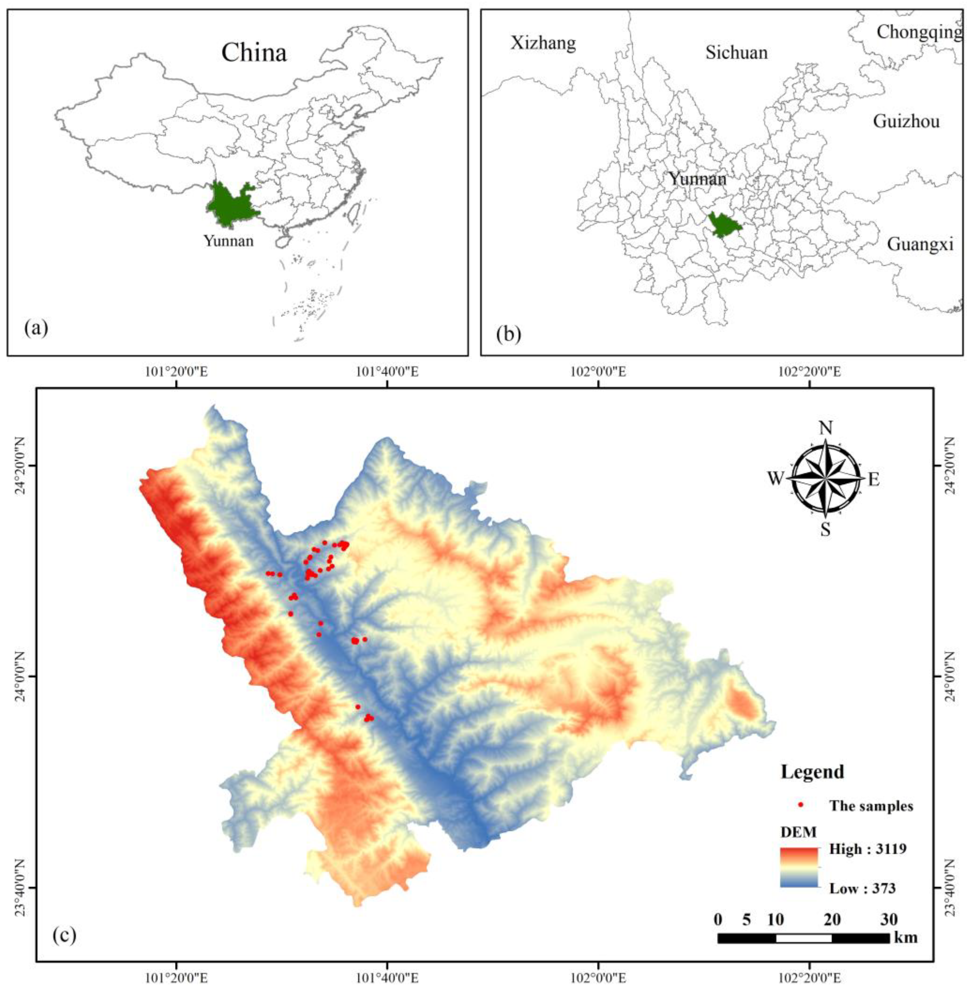
2.1. Description of the Study Area

Xinping Yi and Dai Autonomous County are situated in the southwestern region of Yunnan Province, nestled at the eastern foothills of the Atlas Mountains. It shares borders with Eshan Yi Autonomous County to the east, Shiping County to the southeast, Yuanjiang Hani Yi and Dai Autonomous County to the south, Mojiang Hani Autonomous County to the southwest, Zhenyuan Hani Lahu Autonomous County to the west, and Shuangbai County to the north, with the Lvzhi River serving as the boundary (Figure 1). The county spans an area of 4223 km², with forests covering 2356.71 hectares, constituting 55.8% of the total land area, and the forest coverage rate reached 70.99%. The county’s terrain is elevated in the northwest and declines towards the southeast. The highest elevation is found at Dameyanfeng, the main peak of the Ailao Mountains, reaching 3165.9 m, while the lowest elevation is 422 m, located in Nanhuesun Village, Mosha Town. Influenced by altitude variations, the region exhibits a pronounced vertical climatic gradient, which is classified into three distinct climate types: valley high-temperature zone, mid-mountain warm-temperature zone, and alpine cold-temperature zone. The average annual temperature is 17.4 °C, with an annual rainfall of 946.6 mm. The soil is characterized by a deep, loose structure, and high fertility. The county is home to over 20 genera and approximately 100 species of both naturally occurring and artificially cultivated bamboo. Notably, Dendrocalamus giganteus occupies extensive natural forest areas and exhibits a wide distribution [20].

2.2. Sample Site Survey Data

The field survey for this study was conducted in January 2024. Fifty-one circular plots (r = 12.5 m, s = 490.63 m²) were established based on the principle of representativeness and the ease of surveying the forest area. During the survey, RTK was utilized to pinpoint the coordinates of the central point, and the equipment was maintained in a fixed solution state during data collection. The coordinate consistency was verified through five consecutive collections. Each plot’s diameter at breast height (DBH), plot location, and plant number were meticulously recorded. The calculation of AGC for each plot involved three steps: first, calculating the AGB of a single average standard tree; second, individual AGB was multiplied with carbon content coefficient to obtain individual AGC; and, finally, deriving the plot AGC based on the carbon storage of an individual plant and the number of plants within the plot. The calculation formula is presented as follows:

(1)

The AGB model of Dendrocalamus giganteus was as follows [21]:

Bamboo stalk biomass

$$w=0.145{DBH}^{2.4197},R^2=0.930, P<0.01$$

(1)

Bamboo biomass

$$w=0.0224{DBH}^{2.5286},R^2=0.725, P<0.01$$

(2)

Bamboo leaf biomass

$$w=0.0196{DBH}^{1.917},R^2=0.736,P<0.01$$

(3)

(2)

The AGC calculation formula of Dendrocalamus giganteus was as follows:

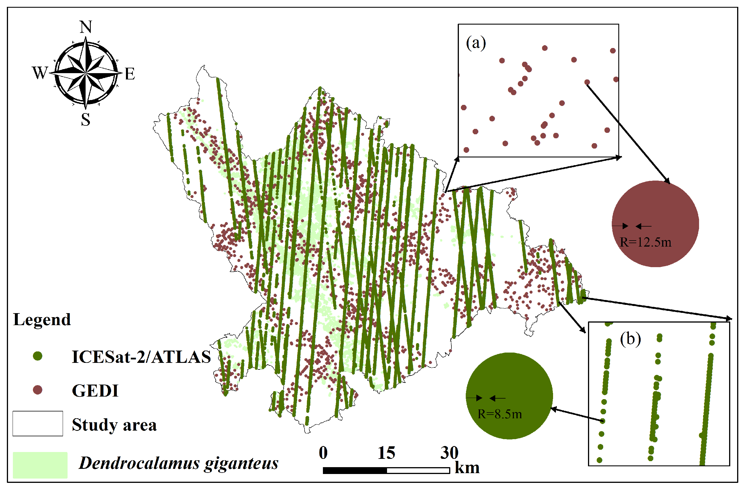
$$C_t=W\times f_c$$

(4)

where C_t is Dendrocalamus giganteus AGC, f_c is carbon coefficient, and the carbon coefficient is 0.45 for bamboo rod, 0.45 for bamboo branch, and 0.43 for bamboo leaf [19].

Among the 51 plots, the minimum value, maximum value, mean value, and standard deviation of Dendrocalamus giganteus (

Table 1. Statistical table of field survey data.

Sample Size (N)	Minimum (Mg/ha)	Maximum (Mg/ha)	Average (Mg/ha)	SD (Mg/ha)
51	4.08	101.78	41.63	20.55

) were 4.08 Mg/ha, 101.78 Mg/ha, 41.63 Mg/ha, and 20.55 Mg/ha, respectively.

2.3. GEDI

On 5 December 2018, the GEDI satellite was successfully deployed to the International Space Station, and it initiated scientific data acquisition in April 2019. The GEDI satellite is equipped with three lasers: two full-power lasers capable of generating two distinct beams each by adjusting the laser beam orientation, and one coverage laser that is split into two beams, thus producing a total of four beams. These three lasers generate eight distinct ground beam tracks, designated as BEAM0000, BEAM0001, BEAM0010, BEAM0011, BEAM0101, BEAM0110, BEAM1000, and BEAM1011. Each ground beam has a footprint diameter of approximately 25 m. The distance between adjacent ground beam tracks is 60 m, while the distance between adjacent ground beam track groups is 600 m, resulting in a total laser track width of 4200 m. GEDI Level 2 products comprise Level 2A and Level 2B. Level 2A primarily provides ground elevation data and relative vegetation elevation metrics. Level 2B predominantly offers forest structural diversity indicators, including vegetation coverage, leaf area index, and vertical leaf profile data [22,23,24]. The research subject of this paper is Dendrocalamus giganteus AGC. The GEDI Level 2B product was downloaded from the official website (https://www.earthdata.nasa.gov/, accessed on 20 January 2024), and the download period was from 1 January 2022 to 20 February 2023, totaling 40 strips. There were 1788 light spots in the study area (Figure 2).

2.4. ICESat-2/ATLAS

The ICESat-2/ATLAS satellite operates with an orbital configuration consisting of three pairs of six beams, and a laser frequency of 10 kHz. It is capable of acquiring multi-beam photon cloud data with an approximate diameter of 17 m and an along-track spacing of 0.7 m. The vertical distance between adjacent orbits is approximately 3 km, while the vertical separation between the strong and weak beams is about 90 m. The satellite revisits the same location every 91 days. The satellite provides 21 data products, categorized into three major types, designated ATL01 to ATL21. This study utilizes two specific data products: ATL03 (global geolocated photon data) and ATL08 (land and vegetation height data) [25]. All ATL03 and ATL08 data products covering the study area were obtained from January 2022 to August 2023 for this study. A total of 44 ATL03 records, comprising 132 orbits and 264 beams, were acquired. Similarly, 44 ATL08 records, also comprising 132 orbits and 264 beams, were obtained. The study data were downloaded from the ICESat-2 website (https://nsidc.org/data/icesat-2/, accessed on 20 January 2024). A total of 21,080 photon spots (Figure 2) were acquired. Following interpolation to derive surface raster information in ArcGIS 10.5, the resolution was resampled to 25 m using the resampling tool.

2.5. Landsat 9

Landsat 9, developed by the USGS and NASA, was successfully launched on 5 November 2021. Following an approximately 100-day commissioning period, the data collected by Landsat 9 became freely accessible worldwide beginning in early 2022. Landsat 9 is equipped with the OLI-2 and TIRS-2 instruments. The OLI-2 instrument captures nine spectral bands across the visible, near-infrared, and mid-infrared spectra, enabling the observation of vegetation, coastal areas, aerosols, water vapor, and clouds. The spatial resolution is 30 m for bands 1 to 7 and 9, 15 m for band 8, and 100 m for bands 10 and 11. The TIRS-2 instrument on Landsat 9 measures thermal infrared radiation from the land surface and outperforms its predecessor, Landsat 8, in both of its bands [26]. This study utilizes Level 1 data from Landsat 9, processed and analyzed via the Google Earth Engine (GEE) platform (http://developers.google.cn/, accessed on 20 January 2024). The download period is from 1 January 2023 to 1 November 2023. The Gram–Schmidt Pan Sharpening Tool was employed to fuse panchromatic images with a spatial resolution of 15 m with multispectral images at 30 m, followed by resampling the fused multispectral images to a resolution of 25 m. The image resolution was adjusted to match the 25 m resolution of GEDI and ICESat-2/ATLAS data, and the feature parameters of single bands and vegetation indices were extracted (Figure 3).

2.6. DEM

This study utilizes a Digital Elevation Model (DEM) with a 12.5 m spatial resolution, derived from the PALSAR sensor aboard the Advanced Land Observing Satellite-1 (ALOS-1). The DEM was resampled to 25 m to ensure compatibility with the resolutions of the GEDI and ICESat-2/ATLAS datasets (Figure 1).

3. Research Methods

The primary steps for estimating the AGC of Dendrocalamus giganteus within the study area, utilizing spaceborne lidar data from GEDI and ICESat-2/ATLAS, are illustrated in Figure 4. These steps include extracting and filtering parameters from GEDI and ICESat-2/ATLAS via Python scripts, downloading Landsat 9 and DEM data using GEE, performing collaborative Kriging interpolation of principal and covariate variables, constructing a regional Stacking model for estimation, evaluating model accuracy, and mapping the spatial distribution of Dendrocalamus giganteus AGC.

3.1. Optimization of Interpolation Variable Features

Before semivariogram analysis, it was imperative to conduct a Pearson correlation analysis on the primary and secondary variables. Constructed utilizing SPSS 27.0 statistical software,

Table 2. Information source variable description and correlation analysis.

Data Source	Variable Name	Description	Cross Variable	Correlation Coefficient
GEDI	c	Total cover, defined as the percentage of the ground covered by the vertical projection of canopy material.	cdem	0.15 **
	f	The foliage height diversity index is calculated by the vertical foliage profile normalized by the total plant area index.	fdem fndvi	0.18 ** 0.07 **
	p	Estimated Pgap(theta) for the selected L2A algorithm.	pdem	−0.15 **
ICESat-2/ATLAS	a	Apparent surface Reflectance.	andvi	−0.23 **
	h1	The 98% height of all the absolute individual canopy heights referenced above the WGS84 ellipsoid.	h1b7	−0.31 **
	h2	The minimum of relative individual canopy heights within the segment. Relative canopy heights have been computed by subtracting the canopy photon height from the estimated terrain surface.	h2b7	−0.30 **
	h3	The median of individual absolute canopy heights within the segment referenced above the WGS84 Ellipsoid.	h3b7	−0.307 **
	h4	Mean of the individual absolute canopy heights within segment referenced above the WGS84 Ellipsoid.	h4b7	−0.306 **
Landsat 9	b7	Short-Wave Infrared 2.
	ndvi	Normalized vegetation index.
ALSO	dem	Elevation.

Note: ** indicates a significant correlation at the 0.01 level; c: cover; f: fhd_normal; p: Pgap_theta; a: asr; h1: h_max_canopy_abs; h2: h_min_canopy; h3: h_median_canopy_abs; h4: h_mean_canopy_abs; c_dem: cover collaborate with dem; f_dem: fhd_normal collaborate with dem; f_ndvi: fhd_normal collaborate with ndvi; p_dem: Pgap_theta collaborate with dem; a_ndvi: asr collaborate with ndvi; h1_b7: h_max_canopy_abs collaborate with b7; h2_b7: h_min_canopy collaborate with b7; h3_b7: h_median_canopy_abs collaborate with b7; h4_b7: h_mean_canopy_abs collaborate with b7.

reveals a highly significant correlation among the variable combinations at the 0.01 level. Variables b7, ndvi, and dem were identified as suitable for co-regionalization. The chosen primary and secondary variables included c_dem, f_dem, f_ndvi, p_dem, and a_ndvi. The correlation coefficients of the other four parameters h1, h2, h3, and h4 with b7 were 0.15, 0.18, 0.07, −0.15, −0.23, −0.31, −0.30, −0.307, and −0.306 in turn.

3.2. Spaceborne Lidar Parameter Interpolation Method

The semi-variation function was also called the “semi-variance function.” The semi-variation function was defined as the value of the regionalized variable Z(x) at points x and x + h, being half of the difference between Z(x) and Z(x + h), which was called the semi-variation function of the regionalized variable Z(x), namely,

$$\mathsf{\gamma }\left(\mathrm{h}\right)={\displaystyle \frac{1}{2N\left(h\right)}}{\sum }_{i=1}^{N\left(h\right)}\left(\right(Z\left(x_i\right)-Z\left(x_i+h\right){)}^2$$

(5)

where r(h) is the semi-variance function value; N(h) is the number of pairs of points in a direction whose distance is equal to h; Z(x_i) is the variable measured at x_i; and Z(x_i + h) is the measurement of x_i’s deviation from h.

3.2.1. Collaborative Kriging Method

CK is a method of linear unbiased optimal estimation using easy-to-obtain variables to cooperate with hard-to-obtain variables, namely,

$$Z^{\mathrm{*}}\left(x_0\right)={\sum }_{i=1}^n{\lambda }_{ai}{Z}_a\left(x_i\right)+{\sum }_{j=1}^m{\lambda }_{bj}{Z}_b\left(x_j\right)$$

(6)

where Z*(x₀) is the estimated value at a certain position; Z_a(x_i) and Z_b(x_j) are the measured values of principal variables and covariables, respectively; λ_ai and λ_bj are the weights of measured values of principal variables Z_a and covariable Z_b; and n and m are the number of measured values of the principal variable and covariate, respectively.

3.2.2. Evaluation of Interpolation Accuracy

This study employed the GS+9.0 software to acquire the optimum semi-variance function model and determined the most suitable model based on the coefficient of determination (R²), residual square sum (RSS), and the ratio of block gold value to base value (SR) [27]. The accuracy of CK was assessed by cross-validation based on the optimal model [28], and the calculation formulas are

$$RSS={\sum }_{i=1}^n{\left(y_i-{\widehat{y}}_i\right)}^2$$

(7)

$$SR={\displaystyle \frac{C_0}{C_0+C}}$$

(8)

$$ME={\displaystyle \frac{\sum _{i-1}^n \left[\stackrel{\wedge }{Z}\left(x_i\right)-Z\left(x_i\right)\right]}{n}}$$

(9)

$$MSE={\displaystyle \frac{\sum _{i-1}^n \left[\stackrel{\wedge }{Z}\right(x_i)-Z(x_i\left)\right]/\stackrel{\wedge }{\sigma }\left(x_i\right)]}{n}}$$

(10)

$$ASE=\sqrt{{\displaystyle \frac{\sum _{i=1}^n \stackrel{\wedge }{\sigma }\left(x_i\right)}{n}}}$$

(11)

$$RMSE=\sqrt{{\displaystyle \frac{\sum _{i=1}^n \left[\stackrel{\wedge }{Z}\right(x_i)-Z(x_i){]}^2}{n}}}$$

(12)

$$RMSSE=\sqrt{{\displaystyle \frac{\sum _{i=1}^n \left\{\left[\stackrel{\wedge }{Z}\right(x_i)-Z(x_i)\right.{]/\left.\stackrel{\wedge }{\sigma }\left(x_i\right)\right\}}^2}{n}}}$$

(13)

where $y_i$ is the measured value, ${\widehat{y}}_i$ is the predicted value, $n$ is the total number of samples, $C_0$ is the nugget value, $C_0+C$ is the sill value, $C$ is the partial sill value, $\stackrel{\wedge }{Z}\left(x_i\right)$ is the predicted value of the i at position x, $Z\left(x_i\right)$ is the observed value of the i at position x, $\stackrel{\wedge }{\sigma }(x_i)$ is the standard error, and n is the number of spots.

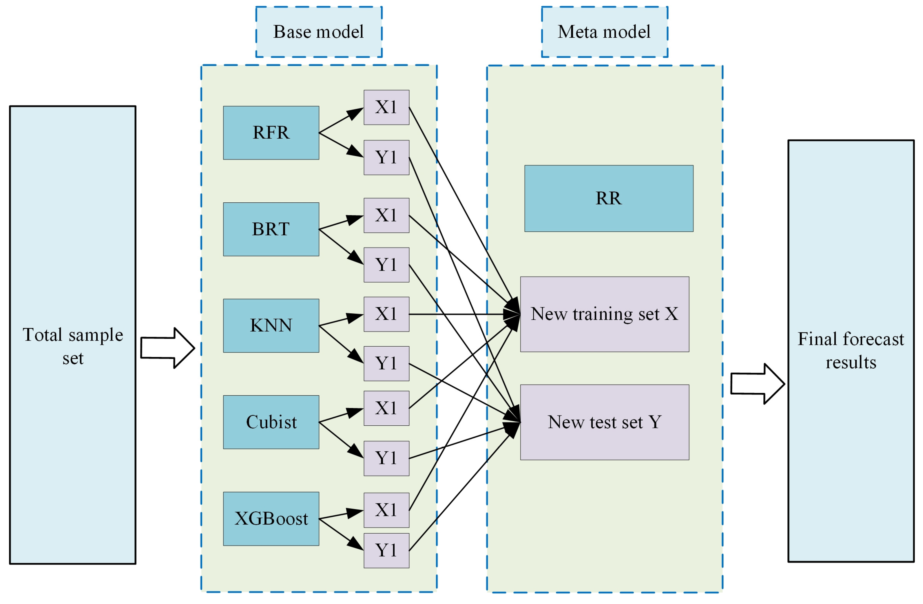
3.3. Dendrocalamus giganteus AGC Stacking-RR Model Establishment and Accuracy Evaluation

Stacking is an integrated learning methodology that integrates multiple distinct learners to achieve superior performance. In Stacking, data are typically trained with multiple base learners, and the predictions generated by these base learners are provided as input to a meta-learner for ultimate predictions [29].

In this research, random forest (RFR), boosted regression trees (BRT), k-nearest neighbor (KNN), Cubist, and extreme gradient boosting (XGBoost) were employed as the base model, and ridge regression (RR) was utilized as the meta-learner to construct the AGC storage model. The technical route map, demonstrated in Figure 5, presents the overall workflow of the study and the correlations among various steps. The main parameters of each data source model are optimized through grid search, and the results are displayed in

Table 3. Shows the grid search results of the main parameters for each data source model.

Data Source	Model	Parameter	Value
GEDI	RFR	mtry, ntree	2, 300
	BRT	n.trees, interaction. depth, shrinkage	10,000, 2, 0.01
	KNN	k-neighbors	2
	Cubist	Committees, neighbor	6, 4
	XGBoost	Nrounds, max_depth, eta	50, 2, 0.1
	RR	lambda	0.1
ICESat-2/ATLAS	RFR	mtry, ntree	2, 300
	BRT	n.trees, interaction. depth, shrinkage	10,000, 10, 0.01
	KNN	k-neighbors	2
	Cubist	Committees, neighbors	6, 4
	XGBoost	Nrounds, max_depth, eta	50, 3, 0.1
	RR	lambda	0.1
GEDI+ICESat-2/ATLAS	RFR	mtry, ntree	5, 1000
	BRT	n.trees, interaction. depth, shrinkage	10,000, 4, 0.01
	KNN	k-neighbors	2
	Cubist	Committees, neighbor	6, 6
	XGBoost	Nrounds, max_depth, eta	80, 2, 0.1
	RR	lambda	0.01

.

3.3.1. Base Model

(1) RFR

Random sampling was conducted through self-aggregation, selecting the optimal features at each node for division. This method has demonstrated a high tolerance for data noise and has effectively mitigated overfitting to a certain extent [30]. Regression modeling using the RFR model was performed with the “randomForest” package in Rstudio (version 4.2.2, Boston, MA, USA), a statistical software environment. In this model, two crucial parameters were configured: the number of trees (ntree) and the number of variables selected at each tree node (mtry).

(2) BRT

For a specified loss function (such as the squared error in regression) and a base predictor, BRT aimed to identify an additive model that minimized the loss function [31]. For regression problems, the BRT model achieved an improved model by employing a weighted average of all base predictors’ outcomes. The BRT model was constructed using the Rstudio (version 4.2.2, Boston, MA, USA) language “gbm” package, and different interaction depths (interaction.depth), shrinkage parameters (shrinkage) and number of trees (n.trees) were selected to tune the model [32].

(3) KNN

KNN is categorized as a lazy machine learning algorithm. The core principle of the kNN algorithm involves identifying the K nearest neighbors of a sample and estimating the result by averaging their attributes. The KNN model was constructed using the “caret” package in the Rstudio (version 4.2.2, Boston, MA, USA) programming language, which includes its algorithm for this purpose. A crucial hyperparameter to be determined is “K”, which specifies the number of nearest neighbors [33].

(4) Cubist

During the construction of the Cubist model, predictors are learned sequentially, with the response variables for each base predictor adjusted based on the previous fitting results. Subsequently, new rules are derived from these adjusted response variables [32]. The Cubist software package in Rstudio (version 4.2.2, Boston, MA, USA) was utilized to set two critical parameters: group size (committees) and the number of neighbors. Committees denote the number of model iterations, while neighbors indicate the number of neighboring points for each sample.

(5) XGBoost

The XGBoost model was designed to prevent overfitting while reducing computational costs by simplifying and regularizing predictions so that they maintained optimal computational efficiency. This was achieved through the simplification and regularization of predictions, ensuring optimal computational efficiency. The fundamental concept involved continuously adding trees and splitting features, learning a new function with each tree addition. Each round of predictions was utilized to fit the residuals of the previous round, predicting the sample score based on its characteristics. Upon completion of the training, where n trees were obtained, each tree was associated with its corresponding leaf node, with each leaf node representing a specific score. Ultimately, the predicted value for the sample was derived by summing the corresponding scores of all trees [34]. In the Rstudio (version 4.2.2, Boston, MA, USA) statistical software environment, the XGBoost package was employed to implement this methodology. Three critical parameters were configured: maximum depth per tree (Nrounds), number of trees (max_depth), and learning rate or step size reduction (eta).

3.3.2. Metamodel

Several studies have demonstrated that excessively intricate meta-models may induce model overfitting, thereby potentially compromising the predictive accuracy of Stacking models [35]. In this study, ridge regression (RR) was utilized as the meta-learner. RR is frequently employed to mitigate multicollinearity issues and represents an extension of the ordinary least squares (OLS) method. By adjusting the coefficient of the regularization term, it regulated the extent to which the coefficients of the feature variables were attenuated [36]. In the Rstudio (version 4.2.2, Boston, MA, USA) language environment, the five trained models of RFR, BRT, KNN, Cubist, and XGBoost were first saved and loaded. Then, when training the RR meta-learner, the grid search method was used to explore the optimal regularization term coefficient. With the aid of RR, the aforementioned basic models were integrated, and, ultimately, a highly performant strong learner was output.

3.3.3. Model Accuracy Evaluation

This study adopted the 10-fold cross-validation strategy. The basic idea of this strategy was to divide the dataset into 10 equal parts. Nine of them were used for training the model and one for testing the model. This process was repeated 10 times, and a different part was selected as the test set each time. Finally, the results of each test were averaged. In the experiment, the fitting effect of the constructed regression model was evaluated through the R², root mean square error (RMSE), and overall estimation accuracy (P). The calculation formulas of each accuracy evaluation index were as follows:

$$R^2=1-{\displaystyle \frac{\sum _{i=1}^n {\left(y_i-{\widehat{y}}_i\right)}^2}{\sum _{i=1}^n {\left(y_i-\overline{y}\right)}^2}}$$

(14)

$$RMSE=\sqrt{{\displaystyle \frac{\sum _{i=1}^n {\left(y_i-{\widehat{y}}_i\right)}^2}{n}}}$$

(15)

$$P=\left(1-{\displaystyle \frac{RMSE}{\overline{y}}}\right)\times 100\mathrm{\%}$$

(16)

where $y_i$ is the actual value; ${\widehat{y}}_i$ is the estimate; $\overline{y }$ is the mean of the estimates; and n is the number of samples.

4. Results

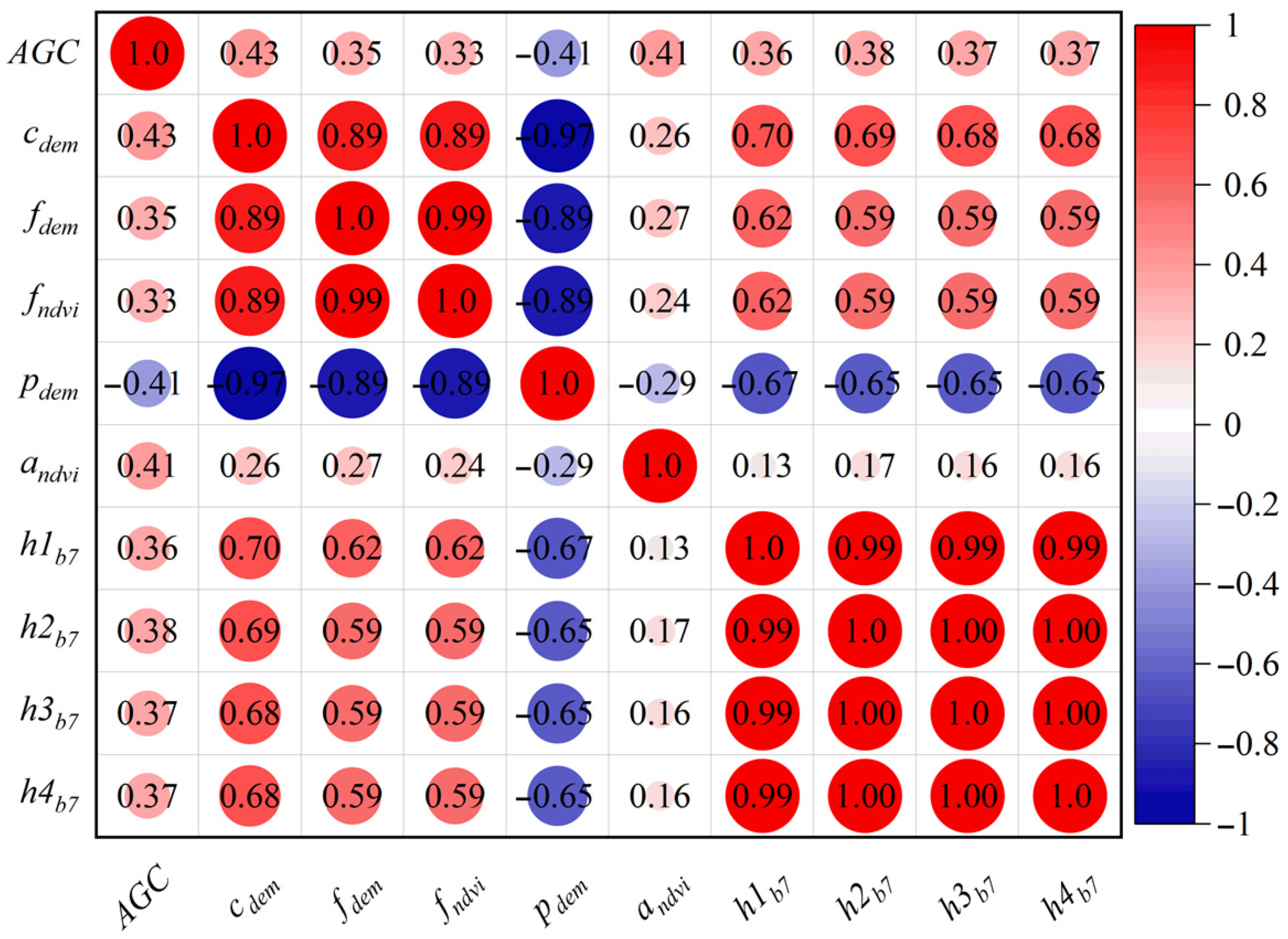
4.1. Correlation Analysis of Model Variables

The extraction of data parameters of GEDI and ICESat-2/ATLAS served as the foundation for establishing the model. Before establishing the regression model, it was indispensable to carry out a correlation analysis of each parameter and screen out the correlated parameters as the independent variable system of the model. With the assistance of the statistical software SPSS 27.0, Pearson correlation analysis was performed on the AGC of the measured sample plot data and the remote sensing variables. Nine variables were found to be correlated, among which four groups of variables were GEDI parameters and five groups were ICESat-2/ATLAS parameters. The parameters of c_dem and p_dem of GEDI were significantly correlated at the 0.01 level, while the parameters of f_dem and f_ndvi were significantly correlated at the 0.05 level. The parameters of a_ndvi, h1_b7, h2_b7, h3_b7, and h4_b7 of ICESat-2/ATLAS were significantly correlated at the 0.01 level. The results are presented in Figure 6. The GEDI correlation coefficients, ranked from largest to smallest in absolute value, were c_dem (0.43) > p_dem (−0.41) > f_dem (0.35) > f_ndvi (0.33), and the ICESat-2/ATLAS correlation coefficients, ranked from largest to smallest in absolute value, were a_ndvi (0.41) > h2_b7 (0.38) > h3_b7 (0.37) and h4_b7 (0.37) > h1_b7 (0.36).

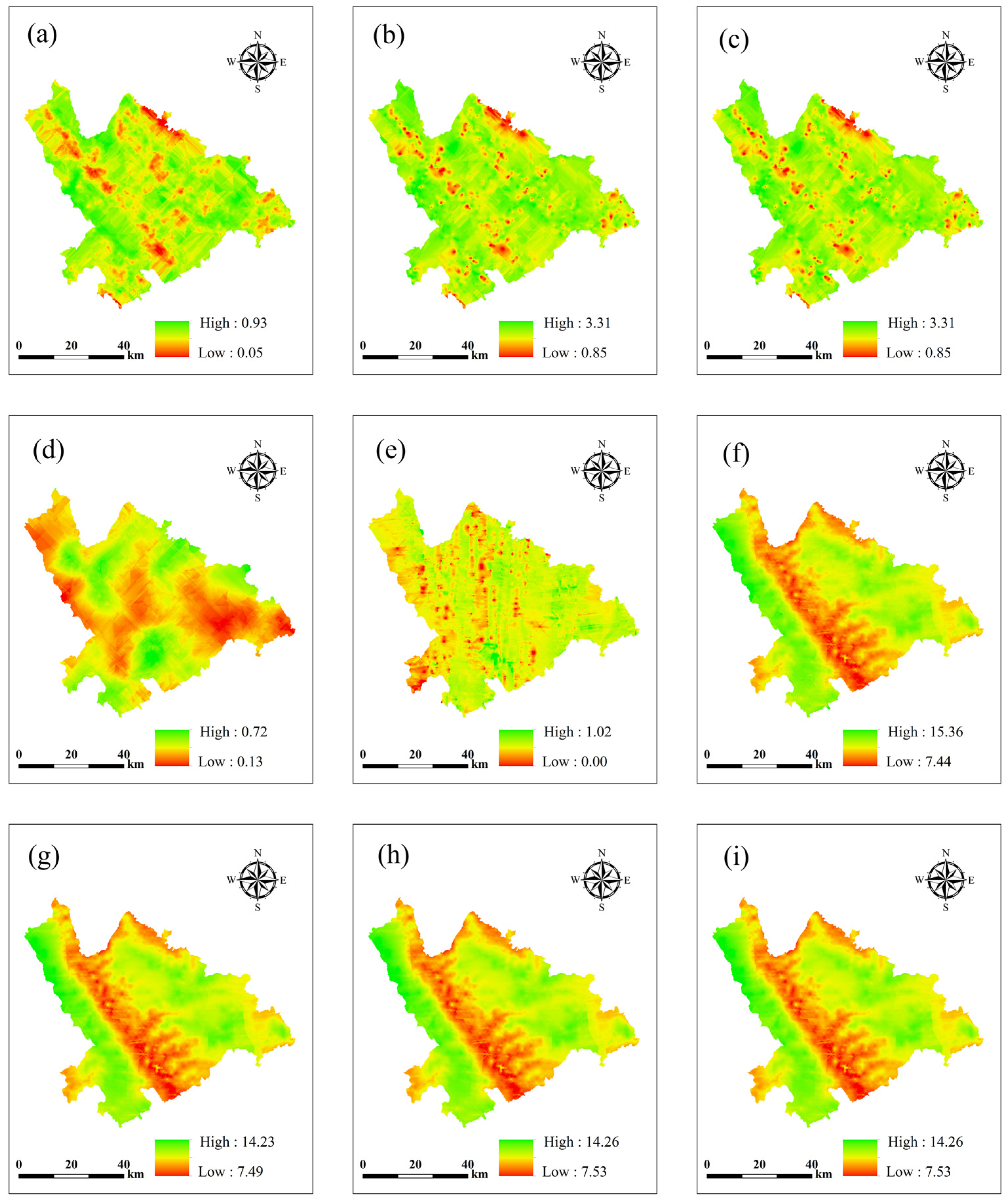
4.2. Interpolation Analysis

The variogram analysis was carried out through the GS+9.0 software, and the model was selected based on the principle of a large R² and a small RSS. SR, the ratio of the nugget value to the sill value, reflects the degree of spatial variation and can describe the strength or weakness of spatial autocorrelation. The smaller the SR, the stronger the spatial autocorrelation. Generally, it can be divided into three grades: 0–25%, 25%–75% [37], and more than 75%, representing the strong, medium, and weak autocorrelation of variables, respectively. The larger the R², the smaller the RSS, and the smaller the SR value, the better the fitting effect. As can be known from

Table 4. Structural analysis of variation function of spot characteristic factors of GEDI and ICESat-2/ATLAS.

Information Source	Modeling Factor	model	C0	C0 + C	SR/%	a/m	RSS	R2
	Cross-variable (cdem)	Gaussian	0.1	53.71	0.19	12,817.18	715	0.82
GEDI + DEM		Spherical	0.1	53.52	0.19	16,100	777	0.81
		Exponential	0.1	53.87	0.19	18,900	1226	0.71
	Cross-variable (fdem)	Gaussian	0.1	93.09	0.11	12,817.18	2298	0.81
GEDI + DEM		Spherical	0.1	92.70	0.11	16,100	2503	0.80
		Exponential	0.1	93.19	0.11	18,600	3933	0.70
	Cross-variable (fndvi)	Gaussian	1.33 × 10−2	0.19	7.05	20,264.99	9.31 × 10−3	0.83
GEDI + Landsat 9		Spherical	1.00 × 10−4	0.19	0.05	24,500	1.01 × 10−2	0.81
		Exponential	1.00 × 10−4	0.20	0.05	32,100	1.38 × 10−2	0.76
	Cross-variable (pdem)	Gaussian	−0.1	−54.87	0.18	12,817.18	681	0.83
GEDI + DEM		Spherical	−0.1	−54.67	0.18	16,100	743	0.82
		Exponential	−0.1	−55.05	0.18	18,900	1205	0.73
	Cross-variable (andvi)	Gaussian	−0.01	−30.65	0.03	14,722.43	308	0.81
ICESat−2/ATLAS + Landsat 9		Spherical	−0.01	−30.46	0.03	18,200	342	0.79
		Exponential	−0.01	−30.6	0.03	21,000	529	0.70
	Cross-variable (h1b7)	Gaussian	−7.70 × 10−3	−3.97 × 10−2	19.40	19,745.38	4.16 × 10−5	0.97
ICESat−2/ATLAS + Landsat 9		Spherical	−4.00 × 10−3	−3.98 × 10−2	10.05	24,500	3.26 × 10−5	0.98
		Exponential	−1.00 × 10−4	−4.07 × 10−2	0.25	27,900	6.49 × 10−5	0.96
	Cross-variable (h2b7)	Gaussian	−7.40 × 10−3	−3.94 × 10−2	18.78	19,918.58	4.04 × 10−5	0.97
ICESat−2/ATLAS + Landsat 9		Spherical	−3.00 × 10−3	−3.95 × 10−2	7.59	24,400	3.21 × 10−5	0.98
		Exponential	−1.00 × 10−4	−4.06 × 10−2	0.25	28,800	6.67 × 10−5	0.97
	Cross-variable (h3b7)	Gaussian	−8.09 × 10−3	−3.97 × 10−2	20.39	24,100	4.00 × 10−5	0.97
ICE−Sat−2/ATLAS + Landsat 9		Spherical	−3.00 × 10−3	−3.97 × 10−2	7.56	24,100	3.26 × 10−5	0.98
		Exponential	−1.00 × 10−4	−4.07 × 10−2	0.25	28,200	6.52 × 10−5	0.96
	Cross-variable (h4b7)	Gaussian	−7.80 × 10−3	−3.96 × 10−2	19.70	19,918.58	4.04 × 10−5	0.97
ICESat−2/ATLAS + Landsat 9		Spherical	−2.90 × 10−3	−3.97 × 10−2	7.30	24,100	3.27 × 10−5	0.98
		Exponential	−1.00 × 10−4	−4.07 × 10−2	0.25	28,200	6.53 × 10−5	0.96

, for the four groups of variables of GEDI (c_dem, f_dem, f_ndvi, p_dem), the Gaussian model was the best, and the SR values were all less than 25%, indicating a strong spatial autocorrelation of the variables. The R² of the Gaussian model for the four groups of variables was the largest, and the RSS was the smallest. Among ICESat-2/ATLAS, for one group of variables (a_ndvi), the Gaussian model was the best, with the largest R² and the smallest RSS, and the SR was within 0–25%. For the other four groups of variables (h1_b7, h2_b7, h3_b7, h4_b7), the spherical model was the best, and the SR was within 0–25%, indicating a strong spatial autocorrelation of the variables. The R² of the spherical model was the largest, and the RSS was the smallest.

The optimal semi-variogram models for the four cross-variables of GEDI (c_dem, f_dem, f_ndvi, p_dem) and one cross-variable of ICESat-2/ATLAS (a_ndvi) were Gaussian models. Their model expressions were as follows:

$$r\left(h\right)=\left\{\begin{array}{c}0 , h=0\\ 0.1+53.61\left(1-e{\displaystyle \frac{h^3}{{\mathrm{12,817.18}}^3}}\right), h>\mathrm{12,817.18}\end{array}\right.$$

(17)

$$r\left(h\right)=\left\{\begin{array}{c}0 , h=0\\ 0.1+92.99\left(1-e{\displaystyle \frac{h^3}{{\mathrm{12,817.18}}^3}}\right), h>\mathrm{12,817.18}\end{array}\right.$$

(18)

$$r\left(h\right)=\left\{\begin{array}{c}0 , h=0\\ 1.33\times {10}^{-2}+0.18\left(1-e{\displaystyle \frac{h^3}{{\mathrm{20,264.99}}^3}}\right), h>\mathrm{20,264.99}\end{array}\right.$$

(19)

$$r\left(h\right)=\left\{\begin{array}{c}0 , h=0\\ -0.1-54.77\left(1-e{\displaystyle \frac{h^3}{{\mathrm{12,817.18}}^3}}\right), h>\mathrm{12,817.18}\end{array}\right.$$

(20)

$$r\left(h\right)=\left\{\begin{array}{c}0 , h=0\\ -0.1-30.64\left(1-e{\displaystyle \frac{h^3}{{\mathrm{14,722.43}}^3}}\right), h>\mathrm{14,722.43}\end{array}\right.$$

(21)

The optimal fitting semi-variogram models for the four cross-variables of ICESat-2/ATLAS (h1_b7, h2_b7, h3_b7, h4_b7) were spherical. Their model expressions were as follows:

$$\mathsf{\gamma }\left(\mathrm{h}\right)=\left\{\begin{array}{c}0 , h=0\\ -2.90\times {10}^{-3}-3.68\times {10}^{-2}\left({\displaystyle \frac{3}{2}}{\displaystyle \frac{h}{\mathrm{24,100}}}-{\displaystyle \frac{1}{2}}{\displaystyle \frac{h^3}{{\mathrm{24,100}}^3}}\right), 0<h\le \mathrm{24,100}\\ -2.90\times {10}^{-3}+3.68\times {10}^{-2} , h>\mathrm{24,100}\end{array}\right.$$

(22)

$$\mathsf{\gamma }\left(\mathrm{h}\right)=\left\{\begin{array}{c}0 , h=0\\ -4.00\times {10}^{-3}-3.58\times {10}^{-2}\left({\displaystyle \frac{3}{2}}{\displaystyle \frac{h}{\mathrm{24,500}}}-{\displaystyle \frac{1}{2}}{\displaystyle \frac{h^3}{{\mathrm{24,500}}^3}}\right), 0<h\le \mathrm{24,500}\\ -4.00\times {10}^{-3}-3.58\times {10}^{-2} , h>\mathrm{24,500}\end{array}\right.$$

(23)

$$\mathsf{\gamma }\left(\mathrm{h}\right)=\left\{\begin{array}{c}0 , h=0\\ -3.00\times {10}^{-3}-3.65\times {10}^{-2}\left({\displaystyle \frac{3}{2}}{\displaystyle \frac{h}{\mathrm{24,400}}}-{\displaystyle \frac{1}{2}}{\displaystyle \frac{h^3}{{\mathrm{24,400}}^3}}\right), 0<h\le \mathrm{24,400}\\ -3.00\times {10}^{-3}-3.65\times {10}^{-2} , h>\mathrm{24,400}\end{array}\right.$$

(24)

$$\mathsf{\gamma }\left(\mathrm{h}\right)=\left\{\begin{array}{c}0 , h=0\\ -3.00\times {10}^{-3}-3.65\times {10}^{-2}\left({\displaystyle \frac{3}{2}}{\displaystyle \frac{h}{\mathrm{24,100}}}-{\displaystyle \frac{1}{2}}{\displaystyle \frac{h^3}{{\mathrm{24,100}}^3}}\right), 0<h\le \mathrm{24,100}\\ -3.00\times {10}^{-3}-3.65\times {10}^{-2} , h>\mathrm{24,100}\end{array}\right.$$

(25)

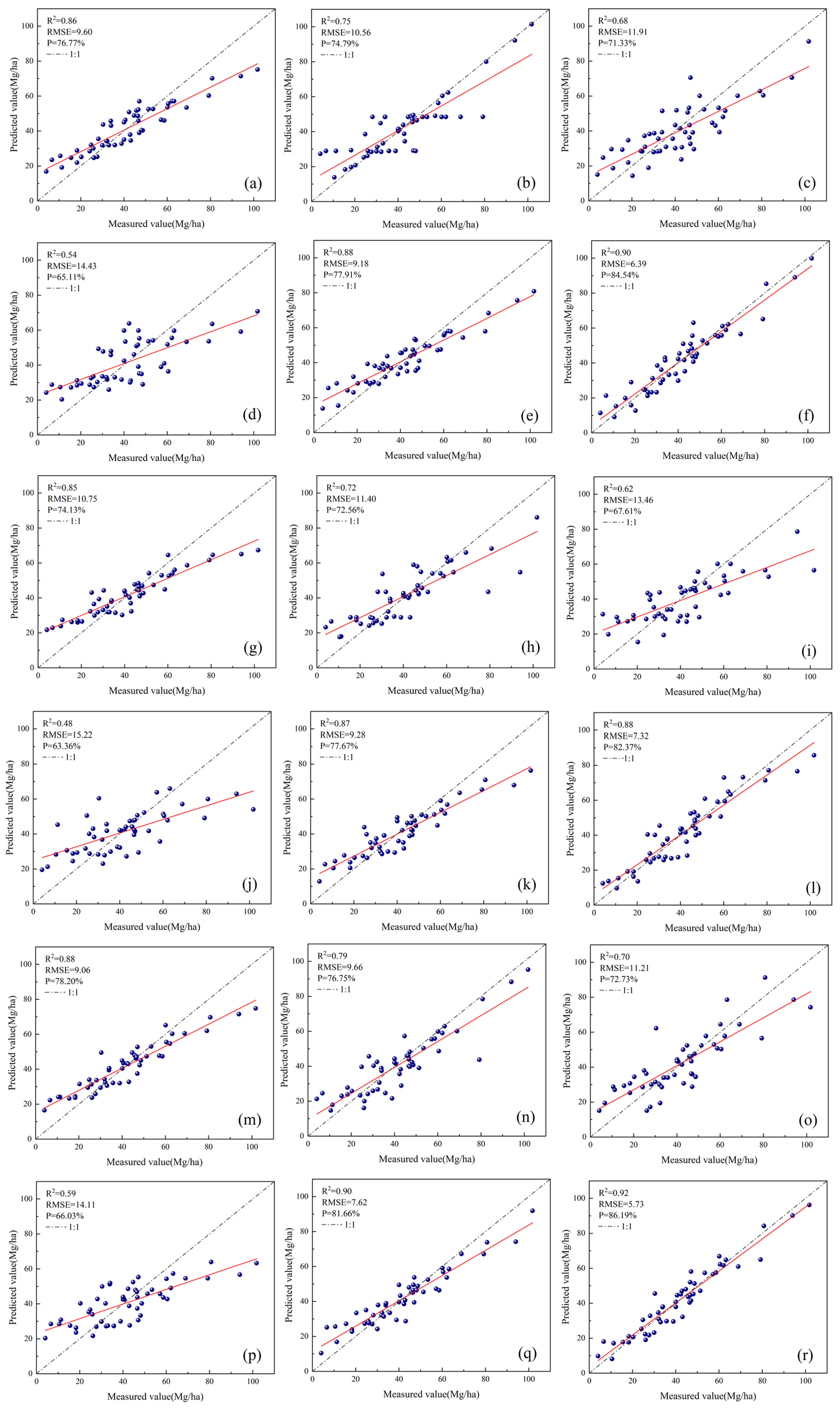
4.3. Interpolation Result Graph and Accuracy Evaluation

As can be seen from Figure 7, the results obtained through the interpolation of different parameters were different. The results obtained by the a_ndvi interpolation of GEDI parameters showed obvious blocky and patchy effects, while the planar data obtained by the interpolation of other parameters presented a smooth state.

When the mean error (ME) and the mean squared error (MSE) were closer to 0, the prediction values were less biased and the accuracy was higher. The closer the values were to 0, the higher the validity of the fitting model, indicating that the CK interpolation was more accurate. When the average standard error (ASE) was greater than the root mean square error (RMSE), the prediction uncertainty was overestimated; conversely, the prediction uncertainty was underestimated. The standardized root mean square error (RMSSE) should approach 1. If its value was greater than 1, the uncertainty of the prediction was underestimated; otherwise, it was overestimated [28].

The cross-validation results are shown in

Table 5. Statistical analysis of cross-validation results.

Modeling Factor	ME	RMSE	MSE	RMSSE	ASE
cdem	0.00	0.31	0.00	0.97	0.32
fdem	0.00	0.53	0.00	0.97	0.54
fndvi	0.00	0.53	0.00	1.00	0.52
pdem	0.00	0.31	0.00	0.97	0.32
andvi	0.00	0.07	−0.01	0.85	0.08
h1b7	0.00	0.31	0.00	1.16	0.26
h2b7	0.00	0.31	0.00	1.15	0.26
h3b7	0.00	0.31	0.00	1.16	0.26
h4b7	0.00	0.30	0.00	1.06	0.29

. Among the parameters of GEDI and ICESat-2/ATLAS, except that the MSE of a_ndvi approached 0, the ME and MSE of other parameters were 0, and the validity of the fitting model was relatively high. The difference between ASE and RMSE of the parameters of GEDI and ICESat-2/ATLAS was 0.01–0.26, the values were close, and the range of RMSSE was 0.85–1.16, approaching 1.

4.4. Model Effect Analysis

Remote sensing factors were screened through Pearson correlation analysis, and RFR, BRT, KNN, Cubist, XGBoost, and Stacking-RR models were established. R², RMSE, and P were employed to evaluate the model accuracy, and the results are presented in Figure 8.

It can be known from Figure 8 that each model had the phenomenon of the overestimation of low values and underestimation of high values to varying degrees. This might be due to the small number of samples with the low and high values of the AGC of Dendrocalamus giganteus, which led to incomplete information contained in the samples. Based on the three evaluation indicators (R², RMSE, and P) of the six models, it was concluded that the Stacking-RR model integrating GEDI and ICESat-2/ATLAS was the best. (1) The order of estimation accuracy of the models using only GEDI from high to low was Stacking-RR (R² = 0.90, RMSE = 6.39 Mg/ha, P = 84.54%) > XGBoost (R² = 0.88, RMSE = 9.18 Mg/ha, P = 77.91%) > RFR (R² = 0.86, RMSE = 9.60 Mg/ha, P = 76.77%) > BRT (R² = 0.75, RMSE = 10.55 Mg/ha, P = 74.79%) > KNN (R² = 0.68, RMSE = 11.91 Mg/ha, P = 71.33%) > Cubist (R² = 0.54, RMSE = 14.43 Mg/ha, P = 65.11%). (2) The order of estimation accuracy of the models using only ICESat-2/ATLAS from high to low was Stacking-RR (R² = 0.88, RMSE = 7.32 Mg/ha, P = 82.37%) > XGBoost (R² = 0.87, RMSE = 9.28 Mg/ha, P = 77.67%) > RFR (R² = 0.85, RMSE = 10.75 Mg/ha, P = 74.13%) > BRT (R² = 0.72, RMSE = 11.40 Mg/ha, P = 72.56%) > KNN (R² = 0.62, RMSE = 13.46 Mg/ha, P = 67.61%) > Cubist (R² = 0.48, RMSE = 15.22 Mg/ha, P = 63.36%). (3) The order of estimation accuracy of the models integrating GEDI and ICESat-2/ATLA from high to low was Stacking-RR (R² = 0.92, RMSE = 5.73 Mg/ha, P = 86.19%) > XGBoost (R² = 0.90, RMSE = 7.62 Mg/ha, P = 81.66%) > RFR (R² = 0.88, RMSE = 9.06 Mg/ha, P = 78.20%) > BRT (R² = 0.79, RMSE = 9.66 Mg/ha, P = 78.20%) > KNN (R² = 0.70, RMSE = 11.21 Mg/ha, P = 72.73%) > Cubist (R² = 0.59, RMSE = 14.11 Mg/ha, P = 66.03%).

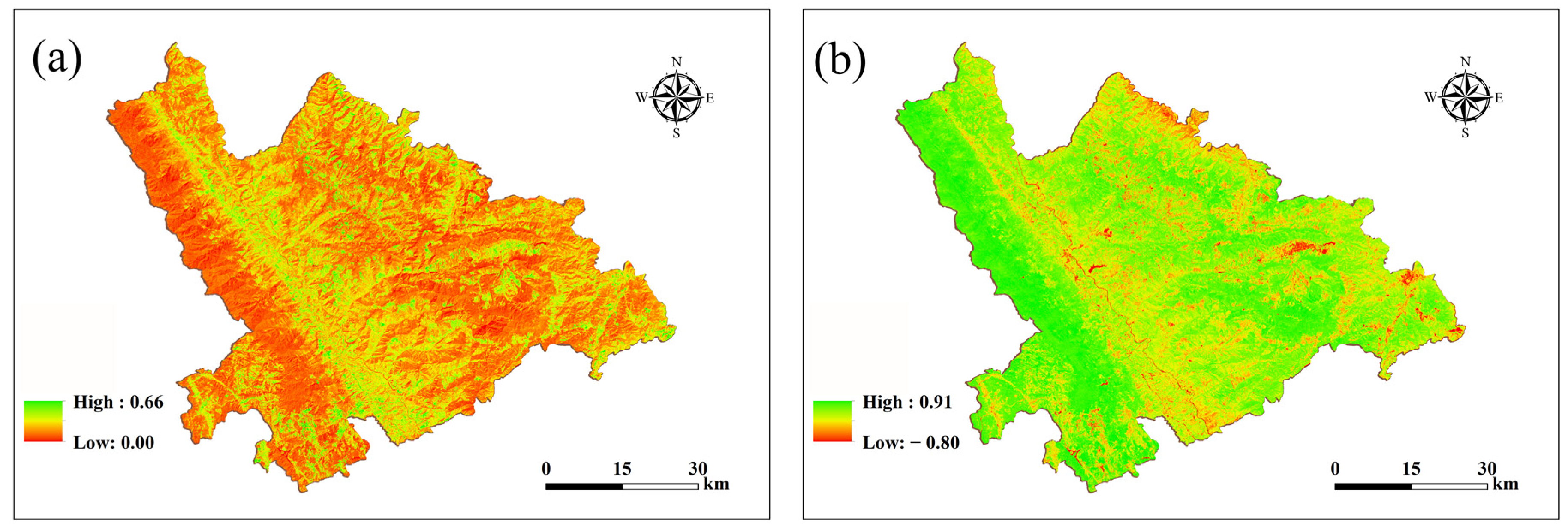
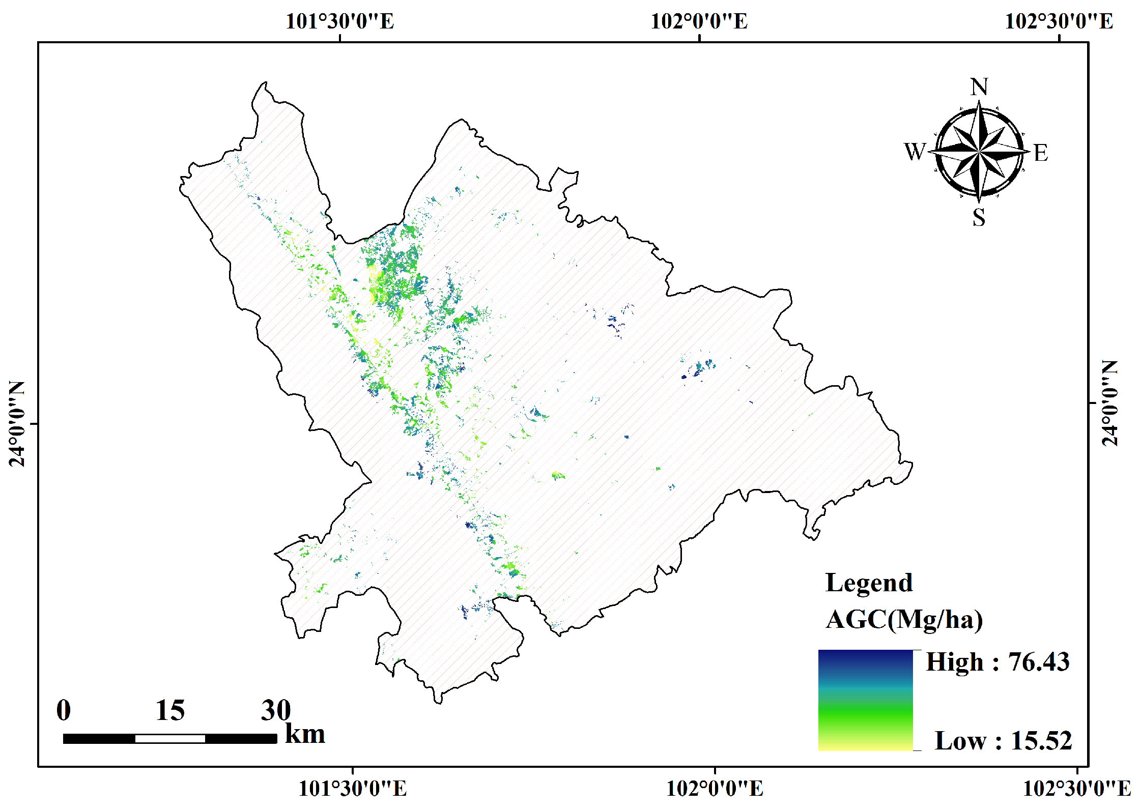
4.5. Spatial Distribution of the AGC Storage of Dendrocalamus giganteus

Based on GEDI and ICESat-2/ATLAS as the main variables, with Landsat 9 and DEM as the auxiliary variables, the grids of CK interpolation were employed as the input variables of the Stacking-RR model to obtain the spatial distribution prediction map of the Dendrocalamus giganteus AGC in Xinping County, as shown in Figure 9. After conducting spatial mapping and classification, the AGC of Dendrocalamus giganteus in the study area was 1.02 × 10⁷ Mg, the average AGC was 43.61 Mg/ha, the maximum value was 76.43 Mg/ha, and the minimum value was 15.52 Mg/ha. It could be seen from the results in the figure that the high-biomass areas of Dendrocalamus giganteus were mainly distributed in the northwest (Gasazhen, Laochangxiang, and Shuitangzhen), and the distribution in other places was more scattered, without obvious regularity. This result was consistent with the distribution of Dendrocalamus giganteus subcompartments in the second-class forest resource survey in 2016.

5. Discussion and Conclusions

5.1. Discussion

5.1.1. Uncertainty Analysis of Data Sources

In recent years, there have been many studies on estimating forest AGC based on spaceborne lidar GEDI and ICESat-2/ATLAS. Generally, the commonly used GEDI and ICESat-2/ATLAS have not eliminated the geographical positioning error caused by lidar spots [25]. Due to the high cost of airborne lidar, it is difficult to achieve forest detection tasks on a regional scale. Some studies indicated [38,39] that the horizontal geolocation accuracy of ICESat-2/ATLAS was less than 5 m, and there was generally a positional error of 2–3 m, while the GEDI data had a positional error of 10.2 m [40]. Compared with ICESat-2/ATLAS, its positioning error in the horizontal direction was more obvious. This could be corrected in the later stage with the help of high-precision airborne lidar data or by using the joint adjustment of stereoscopic images [41]. Meanwhile, the model estimation accuracy of ICESat-2/ATLAS in this study was lower than that of GEDI, which was consistent with the research results of Silva et al. [10]. The reasons for this might first be that ICESat-2/ATLAS adopted photon counting technology, emitted low energy of micro-pulses, and could only receive a few signal photons for each pulse [42], with a short duration and a weak signal [43], being vulnerable to noise and having poor penetration ability through dense tree crowns [10], resulting in difficulties in extracting the tree crown [44] and bringing huge challenges to data processing and estimation. While GEDI was the first full waveform data specifically designed for studying forest structure, its emitted pulse signal had high energy and long duration [42], and GEDI had stronger tree crown penetration ability than ICESat-2/ATLAS [45]. Secondly, in this study, the strong and weak beams of ICESat-2/ATLAS in the study area were not distinguished for research. Existing studies showed [46] that the estimation accuracy of forest aboveground biomass by strong beams was higher than that by weak beams. Therefore, to reduce error transmission, the strong and weak beams could be distinguished in the future to explore their influence on the estimation accuracy of Dendrocalamus giganteus AGC. Additionally, when using the subcompartment attribute data of the second-class forest resource survey in 2016 to screen out the GEDI and ICESat-2/ATLAS spots distributed in the forested land of the study area, there was a problem of inconsistent time, which might lead to a gap between the effective spots screened out and the actual spots, having a certain impact on the accuracy of carbon storage spatial mapping. Regarding Landsat 9, optical images are prone to the light saturation effect in thick forests and are highly influenced by the environment. In this article, additional remote sensing data are added to make up for the deficiencies of optical images, so as to weaken the impact of external environmental factors. The study by Zhao et al. [47] believed that the potential uncertainty of the remote sensing estimation model might be caused by the different temporal, spatial, radiometric, and spectral resolutions of the optical imager. Even at the same time and place, for the same feature object, the feature variable values extracted from the optical image were also different. Based on Landsat 9, this study conducted a correlation analysis of the parameters and variable features of GEDI and ICESat-2/ATLAS and screened out ndvi and b7 as covariates; texture features will be added in the future.

5.1.2. Geostatistical Analysis

This study explores a novel method for obtaining regional-scale AGC estimation that is timely, efficient, cost-effective, and precise, utilizing GEDI and ICESat-2/ATLAS data through spatial interpolation techniques. This method addresses the limitation of discontinuous distribution in GEDI and ICESat-2/ATLAS lidar data by integrating multi-source remote sensing data to produce continuous planar attribute products at the regional scale. This approach offers a new perspective for large-scale or global forest AGC depiction. Spatial interpolation predicts values at unknown locations based on observed values at known locations, effectively leveraging the dense observation data from spaceborne lidar. Liu et al. [48], utilizing the natural neighbor-guided interpolation (NNGI) method, combined GEDI and ICESat-2/ATLAS data to map forest canopy height distribution across the entire area. Compared to GEDI verification footprints, UAV lidar verification data, and field measurements, the R² for forest canopy height after NNGI interpolation ranged from 0.55 to 0.60, with an RMSE between 4.88 and 5.32 m. In this study, GEDI and ICESat-2/ATLAS parameters were used as primary variables, and Landsat 9 and DEM as covariates. The best interpolation model was determined using GS+ software to calculate the semi-variance function, resulting in higher accuracy [49]. Figure 7 illustrates that the eight parameters of CK interpolation display a smooth state, while the a_ndvi of ICESat-2/ATLAS exhibit distinct strip and island distribution characteristics, leading to the underestimation or overestimation of AGC estimates. The interpolation effect of this parameter is consistent with the findings of Yu et al. [50]. Existing studies [37,51] have demonstrated that sequential Gaussian conditional simulation can mitigate the stripe effect. Future work may consider sequential Gaussian simulation interpolation. Additionally, spatial interpolation relies on the “First Law of Geography”, which posits that spatially proximate points are more likely to have similar characteristic values, while distant points are less likely to share similar values [52]. However, the AGC of Dendrocalamus giganteus is influenced by local environmental factors such as climate, moisture, and soil. In future research, factors with strong spatial autocorrelation, such as climate and soil, should be comprehensively considered as covariates for estimation.

5.1.3. Uncertainty Analysis of Stacking-RR Model

In recent years, numerous studies have made use of complementary information from multi-source remote sensing data to enhance the accuracy of forest AGC models. Nevertheless, the estimation of bamboo forest AGC using the Stacking model constructed based on GEDI and ICESat-2/ATLAS data remains insufficiently explored. Schwenker [53] suggested that the accuracy of a single model was insufficient to effectively utilize all available information, as each algorithm had distinct advantages and disadvantages, leading to various uncertainties in model errors. Therefore, integrating multiple base learners is necessary. The Stacking model integrates the strengths of various learning models, thereby enhancing performance robustness, reducing estimation uncertainty, and improving predictive accuracy [54]. In this study, we employed Pearson correlation analysis to identify variables associated with AGC from an extensive set of remote sensing features. We integrated five machine learning models and utilized RR as the meta-learner to develop a remote sensing estimation model for the AGC of Dendrocalamus giganteus using Stacking-RR ensemble learning. Our results demonstrate that the Stacking-RR ensemble model enhances R² and p values while reducing RMSE. This model outperforms individual machine learning models and aligns with previous findings [55]. Previous studies have highlighted the importance of selecting appropriate base learners for the efficacy of the Stacking model. Combining diverse base learners enhances the ability to correct errors inherent in single models and mitigates the dependence on sample size [56]. Choosing an appropriate number and type of base learners is also better than randomly selecting base learners to construct an accurate Stacking model [57]. In this study, five models were directly integrated. In the future, indicators such as correlation coefficient, covariance, difference measure, chi-square measure, and mutual information could be used to measure the diversity of base learners in Stacking [58]. Moreover, the meta-learner used to fit the base learners would also affect the performance of the Stacking model [57]. Huang [59] et al. compared the performance of 11 machine learning algorithms and selected XGBoost as the optimal meta-model for Stacking integration, which improved model accuracy. Therefore, in the future, the best meta-learner can be further optimized and selected to improve the accuracy of the estimation of Dendrocalamus giganteus AGC. In addition, in non-parametric model building, the optimization of model parameters is particularly important. The uncertainty of remote sensing models and model parameters has a significant impact on the accuracy of estimation results [60]. For the different information sources, forest types, and spatial distributions of biomass and carbon stocks, the applicability of the values of model parameters was inconsistent [3]. The approach proposed in this study for estimating the AGC of Dendrocalamus giganteus through the integration of GEDI and ICESat-2/ATLAS data and the combination of the Stacking-RR model can effectively enhance the model’s accuracy, reduce errors, and lower costs. This also offers an example of fusing multiple data and models for the inversion of bamboo forest parameters at the regional scale.

5.2. Conclusions

Lidar can penetrate forest canopy and obtain more accurate vertical structure information, which has great potential for improving the accuracy of forest AGC estimation. In this study, we used preprocessed GEDI and ICESat-2/ATLAS data as primary variables, supplemented by Landsat 9 and DEM data as auxiliary variables. We employed co-Kriging interpolation for spatial expansion and estimated the AGC of Dendrocalamus giganteus using Stacking-RR, XGBoost, RFR, BRT, KNN, and Cubist models. The results indicated that Gaussian models best fitted the semi-variograms for c_dem, f_dem, f_ndvi, p_dem, and a_ndvi. Spherical models best fitted the semi-variograms for h1_b7, h2_b7, h3_b7, and h4_b7. Separate models were established based on the parameters from GEDI and ICESat-2/ATLAS. The GEDI model outperformed the ICESat-2/ATLAS model in estimation accuracy. The integrated Stacking-RR model combining GEDI and ICESat-2/ATLAS data achieved superior estimation accuracy (R² = 0.92, RMSE = 5.73 Mg/ha, p = 86.19%) compared to single models: XGBoost (R² = 0.90, RMSE = 7.62 Mg/ha, p = 81.66%), RFR (R² = 0.88, RMSE = 9.06 Mg/ha, p = 78.20%), BRT (R² = 0.79, RMSE = 9.66 Mg/ha, p = 78.20%), KNN (R² = 0.70, RMSE = 11.21 Mg/ha, p = 72.73%), and Cubist (R² = 0.59, RMSE = 14.11 Mg/ha, p = 66.03%).

The research shows that integrating GEDI, ICESat-2/ATLAS data, combined with the Stacking-RR model to estimate the AGC storage of Dendrocalamus giganteus can improve the accuracy of the model and reduce the error, which can provide a reference for the inversion of bamboo forest parameters by fusing various data and models at the regional scale.

References

1. Avitabile, V.; Herold, M.; Heuvelink, G.B.; Lewis, S.L.; Phillips, O.L.; Asner, G.P.; Armston, J.; Ashton, P.S.; Banin, L.; Bayol, N. An integrated pan-tropical biomass map using multiple reference datasets. Glob. Chang. Biol. 2016, 22, 1406–1420. [Google Scholar] [CrossRef]
2. Shu, Q.; Xi, L.; Wang, K.; Xie, F.; Pang, Y.; Song, H. Optimization of samples for remote sensing estimation of forest aboveground biomass at the regional scale. Remote Sens. 2022, 14, 4187. [Google Scholar] [CrossRef]
3. Lu, D.; Chen, Q.; Wang, G.; Liu, L.; Li, G.; Moran, E. A survey of remote sensing-based aboveground biomass estimation methods in forest ecosystems. Int. J. Digit. Earth 2016, 9, 63–105. [Google Scholar] [CrossRef]
4. Ou, G.; Li, C.; Lv, Y.; Wei, A.; Xiong, H.; Xu, H.; Wang, G. Improving aboveground biomass estimation of Pinus densata forests in Yunnan using Landsat 8 imagery by incorporating age dummy variable and method comparison. Remote Sens. 2019, 11, 738. [Google Scholar] [CrossRef]
5. Li, B.; Wang, W.; Bai, L.; Chen, N.; Wang, W. Estimation of aboveground vegetation biomass based on Landsat-8 OLI satellite images in the Guanzhong Basin, China. Int. J. Remote Sens. 2019, 40, 3927–3947. [Google Scholar] [CrossRef]
6. Han, H.; Wan, R.; Li, B. Estimating forest aboveground biomass using Gaofen-1 images, Sentinel-1 images, and machine learning algorithms: A case study of the Dabie Mountain Region, China. Remote Sens. 2021, 14, 176. [Google Scholar] [CrossRef]
7. Gleason, C.J.; Im, J. Forest biomass estimation from airborne LiDAR data using machine learning approaches. Remote Sens. Environ. 2012, 125, 80–91. [Google Scholar] [CrossRef]
8. Magdon, P.; González-Ferreiro, E.; Pérez-Cruzado, C.; Purnama, E.S.; Sarodja, D.; Kleinn, C. Evaluating the potential of ALS data to increase the efficiency of aboveground biomass estimates in tropical peat–swamp forests. Remote Sens. 2018, 10, 1344. [Google Scholar] [CrossRef]
9. Duncanson, L.; Kellner, J.R.; Armston, J.; Dubayah, R.; Minor, D.M.; Hancock, S.; Healey, S.P.; Patterson, P.L.; Saarela, S.; Marselis, S. Aboveground biomass density models for NASA’s Global Ecosystem Dynamics Investigation (GEDI) lidar mission. Remote Sens. Environ. 2022, 270, 112845. [Google Scholar] [CrossRef]
10. Silva, C.A.; Duncanson, L.; Hancock, S.; Neuenschwander, A.; Thomas, N.; Hofton, M.; Fatoyinbo, L.; Simard, M.; Marshak, C.Z.; Armston, J. Fusing simulated GEDI, ICESat-2 and NISAR data for regional aboveground biomass mapping. Remote Sens. Environ. 2021, 253, 112234. [Google Scholar] [CrossRef]
11. Xu, X.; Zhou, G.; Du, H.; Dong, D.; Cui, R.; Zhou, Y.; Shen, Z. Estimation of Aboveground Biomass of Phyllostachys praecox Forest Based on Landsat Thematic Mapper. Sci. Silvae Sin. 2011, 47, 1–6. [Google Scholar]
12. Chen, Y.; Li, L.; Lu, D.; Li, D. Exploring bamboo forest aboveground biomass estimation using Sentinel-2 data. Remote Sens. 2018, 11, 7. [Google Scholar] [CrossRef]
13. Wang, J. Remote Sensing Estimation of Bamboo Forest Aboveground Carbon Storage Based on Ensemble Learning. Master’s Thesis, Zhejiang A&F University, Hangzhou, China, 2022. [Google Scholar]
14. Hu, X.; Zhang, P.; Zhang, Q.; Wang, J. Improving wetland cover classification using artificial neural networks with ensemble techniques. GIScience Remote Sens. 2021, 58, 603–623. [Google Scholar] [CrossRef]
15. Du, C.; Fan, W.; Ma, Y.; Jin, H.-I.; Zhen, Z. The effect of synergistic approaches of features and ensemble learning algorithms on aboveground biomass estimation of natural secondary forests based on ALS and Landsat 8. Sensors 2021, 21, 5974. [Google Scholar] [CrossRef] [PubMed]
16. Li, X.; Zhang, M.; Long, J.; Lin, H. A novel method for estimating spatial distribution of forest above-ground biomass based on multispectral fusion data and ensemble learning algorithm. Remote Sens. 2021, 13, 3910. [Google Scholar] [CrossRef]
17. Wang, J.; Du, H.; Li, X.; Mao, F.; Zhang, M.; Liu, E.; Ji, J.; Kang, F. Remote sensing estimation of bamboo forest aboveground biomass based on geographically weighted regression. Remote Sens. 2021, 13, 2962. [Google Scholar] [CrossRef]
18. Xiao, X.; Bian, J.; Peng, X.-P.; Xu, H.; Xiao, B.; Sun, R.-C. Autohydrolysis of bamboo (Dendrocalamus giganteus Munro) culm for the production of xylo-oligosaccharides. Bioresour. Technol. 2013, 138, 63–70. [Google Scholar] [CrossRef]
19. Teng, J. Carbon Storage and Energy of Typical Sympodial Bamboo Ecosystems in China. Master’s Thesis, Zhejiang A&F University, Hangzhou, China, 2016. [Google Scholar]
20. Yun, P.; Liu, Q. Economic Bamboo Species Resources and Development and Utilization Countermeasures in Xinping County. J. Southwest For. Univ. Nat. Sci. 2007, 27, 63–66. [Google Scholar]
21. Keren, W.; Wenxiu, L.; Qingtai, S.; Hongbin, L.; Hongyan, L.; Dan, S.; Qiang, W.; Hongying, Z. Analysis of Moisture Content and Construction of Aboveground Biomass Regression Model for Dendrocalamus giganteus Plantation. J. Southwest For. Univ. Nat. Sci. 2021, 41, 168–174. [Google Scholar]
22. Han, M.; Xing, Y.; Li, G.; Huang, J.; Cai, L.J. Comparison of the accuracy of the maximum canopy height and biomass inversion of the data of different GEDI algorithm groups. J. Cent. South Univ. For. Technol. 2022, 42, 72–82. [Google Scholar]
23. Liu, L.; Wang, C.; Nie, S.; Zhu, X.; Xi, X.; Wang, J. Analysis of the influence of different algorithms of GEDI L2A on the accuracy of ground elevation and forest canopy height. J. Univ. Chin. Acad. Sci. 2022, 39, 502. [Google Scholar]
24. Coyle, D.B.; Stysley, P.R.; Poulios, D.; Clarke, G.B.; Kay, R.B. Laser transmitter development for NASA’s Global Ecosystem Dynamics Investigation (GEDI) lidar. In Lidar Remote Sensing for Environmental Monitoring XV; SPIE: Bellingham, WA, USA, 2015; pp. 19–25. [Google Scholar]
25. Song, H.; Xi, L.; Shu, Q.; Wei, Z.; Qiu, S. Estimate forest aboveground biomass of mountain by ICESat-2/ATLAS data interacting cokriging. Forests 2022, 14, 13. [Google Scholar] [CrossRef]
26. Jiang, F.; Sun, H.; Chen, E.; Wang, T.; Cao, Y.; Liu, Q. Above-ground biomass estimation for coniferous forests in Northern China using regression kriging and landsat 9 images. Remote Sens. 2022, 14, 5734. [Google Scholar] [CrossRef]
27. Su, H.; Shen, W.; Wang, J.; Ali, A.; Li, M. Machine learning and geostatistical approaches for estimating aboveground biomass in Chinese subtropical forests. For. Ecosyst. 2020, 7, 64. [Google Scholar] [CrossRef]
28. Lu, M. Distribution of Forest Biomass for Main Forest Types in Tahe Forestry Administration of Daxinganling Based on Geostatistics. Master’s Thesis, Northeast Forestry University, Harbin, China, 2017. [Google Scholar]
29. Zhang, Y.; Ma, J.; Liang, S.; Li, X.; Liu, J. A stacking ensemble algorithm for improving the biases of forest aboveground biomass estimations from multiple remotely sensed datasets. GIScience Remote Sens. 2022, 59, 234–249. [Google Scholar] [CrossRef]
30. Belgiu, M.; Drăguţ, L. Random forest in remote sensing: A review of applications and future directions. ISPRS J. Photogramm. Remote Sens. 2016, 114, 24–31. [Google Scholar] [CrossRef]
31. Servia, H.; Pareeth, S.; Michailovsky, C.I.; de Fraiture, C.; Karimi, P. Operational framework to predict field level crop biomass using remote sensing and data driven models. Int. J. Appl. Earth Obs. Geoinf. 2022, 108, 102725. [Google Scholar] [CrossRef]
32. Ou, Q.; Li, H.; Lei, X.; Yang, Y. Difference analysis in estimating biomass conversion and expansion factors of masson pine in Fujian Province, China based on national forest inventory data: A comparison of three decision tree models of ensemble learning. Chin. J. Appl. Ecol. 2018, 29, 2007–2016. [Google Scholar] [CrossRef]
33. Fu, X.; Chang, Q.; Zhang, Y.; Zhang, Z.; Zheng, Z.; Li, K. Estimation of kiwifruit leaf chlorophyll content based on Stacking ensemble learning. Agric. Res. Arid Areas 2023, 41, 247–256. [Google Scholar]
34. Tan, Y.; Tian, Y.; Huang, Z.; Zhang, Q.; Tao, J.; Liu, H.; Yang, Y.; Zhang, Y.; Lin, J.; Deng, J. Aboveground biomass of Sonneratia apetala mangroves in Mawei Sea of Beibu Gulf based on XGBoost machine learning algorithm. Acta Ecol. Sin. 2023, 43, 4674–4688. [Google Scholar]
35. Li, Y.; Huang, W.; Xi, J. NOx Emission Forecasting based on Stacking Ensemble Model. J. Eng. Therm. Energy Power 2021, 36, 73–81. [Google Scholar] [CrossRef]
36. Fu, X. Study on Estimation of Physiological and Biochemical Parameters of Kiwifruit Based on Stacking Ensemble Learning. Master’s Thesis, Northwest A&F University, Xianyang, China, 2023. [Google Scholar]
37. Luo, S.; Xu, L.; Yu, J.; Zhou, W.; Yang, Z.; Wang, S.; Guo, C.; Gao, Y.; Xiao, J.; Shu, Q. Sampling Estimation and Optimization of Typical Forest Biomass Based on Sequential Gaussian Conditional Simulation. Forests 2023, 14, 1792. [Google Scholar] [CrossRef]
38. Liu, A.; Cheng, X.; Chen, Z. Performance evaluation of GEDI and ICESat-2 laser altimeter data for terrain and canopy height retrievals. Remote Sens. Environ. 2021, 264, 112571. [Google Scholar] [CrossRef]
39. Neuenschwander, A.; Pitts, K.; Jelley, B.; Robbins, J.; Klotz, B.; Popescu, S.; Nelson, R.; Harding, D.; Pederson, D.; Sheridan, R. ATLAS/ICESat-2 L3A Land and Vegetation Height, Version 5; NASA National Snow and Ice Data Center Distributed Active Archive Center: Boulder, CO, USA, 2021. [Google Scholar]
40. Wang, J.; Shen, X.; Cao, L. Upscaling Forest Canopy Height Estimation Using Waveform-Calibrated GEDI Spaceborne LiDAR and Sentinel-2 Data. Remote Sens. 2024, 16, 2138. [Google Scholar] [CrossRef]
41. Nan, Y. Research on Key Technologies of Active and Passive Fusion Topography Surveying with Photon Counting Laser Altimeter. Ph.D. Thesis, University of Electronic Science and Technology of China, Chengdu, China, 2022. [Google Scholar]
42. Zhu, X.; Nie, S.; Wang, C.; Xi, X.; Lao, J.; Li, D. Consistency analysis of forest height retrievals between GEDI and ICESat-2. Remote Sens. Environ. 2022, 281, 113244. [Google Scholar] [CrossRef]
43. Zhu, X. Forest Height Retrieval of China with a Resolution of 30 m Using ICESat-2 and GEDI Data; Aerospace Information Research Institute, Chinese Academy of Sciences (CAS): Beijing, China, 2021. [Google Scholar]
44. Neuenschwander, A.; Guenther, E.; White, J.C.; Duncanson, L.; Montesano, P. Validation of ICESat-2 terrain and canopy heights in boreal forests. Remote Sens. Environ. 2020, 251, 112110. [Google Scholar] [CrossRef]
45. Sothe, C.; Gonsamo, A.; Lourenço, R.B.; Kurz, W.A.; Snider, J. Spatially continuous mapping of forest canopy height in Canada by combining GEDI and ICESat-2 with PALSAR and Sentinel. Remote Sens. 2022, 14, 5158. [Google Scholar] [CrossRef]
46. Narine, L.L.; Popescu, S.C.; Malambo, L. Using ICESat-2 to estimate and map forest aboveground biomass: A first example. Remote Sens. 2020, 12, 1824. [Google Scholar] [CrossRef]
47. Zhao, P.; Lu, D.; Wang, G.; Wu, C.; Huang, Y.; Yu, S. Examining spectral reflectance saturation in Landsat imagery and corresponding solutions to improve forest aboveground biomass estimation. Remote Sens. 2016, 8, 469. [Google Scholar] [CrossRef]
48. Liu, X.; Su, Y.; Hu, T.; Yang, Q.; Liu, B.; Deng, Y.; Tang, H.; Tang, Z.; Fang, J.; Guo, Q. Neural network guided interpolation for mapping canopy height of China’s forests by integrating GEDI and ICESat-2 data. Remote Sens. Environ. 2022, 269, 112844. [Google Scholar] [CrossRef]
49. Xu, L.; Shu, Q.; Fu, H.; Zhou, W.; Luo, S.; Gao, Y.; Yu, J.; Guo, C.; Yang, Z.; Xiao, J. Estimation of Quercus biomass in Shangri-La based on GEDI spaceborne LiDAR data. Forests 2023, 14, 876. [Google Scholar] [CrossRef]
50. Yu, J.; Lai, H.; Xu, L.; Luo, S.; Zhou, W.; Song, H.; Xi, L.; Shu, Q. Estimation of Forest Canopy Cover by Combining ICESat-2/ATLAS Data and Geostatistical Method/Co-Kriging. IEEE J. Sel. Top. Appl. Earth Obs. Remote Sens. 2023, 17, 1824–1838. [Google Scholar] [CrossRef]
51. Liu, L.; Wang, H.; Dai, W.; Yang, X.; Li, X. Spatial heterogeneity of soil organic carbon and nutrients in low mountain area of Changbai Mountains. Yingyong Shengtai Xuebao 2014, 25, 2460–2468. [Google Scholar]
52. Feng, J.; Wu, X.; Li, D.; Zhou, X. Application of spatial statistical analysis methods and related analytic softwares in research of infectious diseases. Chin. J. Schistosomiasis Control 2011, 23, 217. [Google Scholar]
53. Schwenker, F. Ensemble methods: Foundations and algorithms [book review]. IEEE Comput. Intell. Mag. 2013, 8, 77–79. [Google Scholar] [CrossRef]
54. Tang, Z.; Xia, X.; Huang, Y.; Lu, Y.; Guo, Z. Estimation of national forest aboveground biomass from multi-source remotely sensed dataset with machine learning algorithms in China. Remote Sens. 2022, 14, 5487. [Google Scholar] [CrossRef]
55. Naimi, A.I.; Balzer, L.B. Stacked generalization: An introduction to super learning. Eur. J. Epidemiol. 2018, 33, 459–464. [Google Scholar] [CrossRef] [PubMed]
56. Breiman, L. Stacked regressions. Mach. Learn. 1996, 24, 49–64. [Google Scholar] [CrossRef]
57. Chen, Y.; Ma, L.; Yu, D.; Feng, K.; Wang, X.; Song, J. Improving leaf area index retrieval using multi-sensor images and stacking learning in subtropical forests of China. Remote Sens. 2021, 14, 148. [Google Scholar] [CrossRef]
58. Dutta, H. Measuring Diversity in Regression Ensembles. In Proceedings of the 4th Indian International Conference on Artificial Intelligence, IICAI, Tumkur, Karnataka, India, 16–18 December 2009. 17p. [Google Scholar]
59. Huang, T.; Ou, G.; Xu, H.; Zhang, X.; Wu, Y.; Liu, Z.; Zou, F.; Zhang, C.; Xu, C. Comparing Algorithms for Estimation of Aboveground Biomass in Pinus yunnanensis. Forests 2023, 14, 1742. [Google Scholar] [CrossRef]
60. Fu, Y.; Lei, Y.; Zeng, W. Uncertainty analysis for regional-level above-ground biomass estimates based on individual tree biomass model. Acta Ecol. Sin. 2015, 35, 7738–7747. [Google Scholar]
Figure 1. Overview of the study area: (a) The study area is located in southwest China, (b) Xinping is part of Yunnan Province, and (c) Xinping DEM, the red circle, is a collection of 51 Dendrocalamus giganteus plots.
Forests 15 01440 g001
Figure 2. Schematic diagram of GEDI and ICESat-2/ATLAS spots in the study area: (a) GEDI spots, (b) ICESat-2/ATLAS spots.
Forests 15 01440 g002
Figure 3. Landsat 9: (a) b7, (b) ndvi. Note: b7: Short-Wave Infrared 2. ndvi: Normalized vegetation index.
Forests 15 01440 g003
Figure 4. Technology roadmap.
Forests 15 01440 g004
Figure 5. Model technology roadmap.
Forests 15 01440 g005
Figure 6. Correlation matrix between AGC and remote sensing factors.
Forests 15 01440 g006
Figure 7. Interpolation result: (a) is cdem, (b) fdem, (c) fndvi, (d) pdem, (e) andvi, (f) h1b7, (g) h2b7, (h) h3b7, and (i) h4b7.
Forests 15 01440 g007
Figure 8. Scatter diagram of the AGC model of Dendrocalamus giganteus. The models are RFR, BRT, KNN, Cubist, XGBoost, and Stacking-RR. GEDI model (af), ICESat-2/ATLAS model (gl), integrated GEDI and ICESat-2/ATLAS model (mr).
Forests 15 01440 g008
Figure 9. Distribution map of Dendrocalamus giganteus AGC in Xinping County.
Forests 15 01440 g009