Abstract
Annual urban forest expansion dynamics are crucial for assessing the benefits and potential issues associated with vegetation accumulation over time. LandTrendr (Landsat-Based Detection of Trends in Disturbance and Recovery) can efficiently detect the dynamics of interannual land cover change, but it has difficulty distinguishing urban forest expansion from urban surface rapid conversions, as changes are usually filtered by magnitude-of-change thresholds. To accurately detect annual urban forest expansion dynamics, we developed an improved method using random forest-supervised classification to filter urban forests. We further enhanced the performance of the improved method by incorporating trend features between segments. Additionally, we tested two threshold-based filtering baseline methods. These methods were tested with various spectral and parameter combinations in Beijing’s Central District and the 1st Greenbelt from 1994 to 2022. The improved method with trend features achieved the highest average accuracy of 89.35%, representing a 25% improvement over baseline methods. Post-change trend features aided in accurate identification, while quantitative features rather than extremum features were more important in filtering. The improved method with trend features tested in Beijing’s 2nd Greenbelt also showed an accuracy of 88.27%, confirming its stability. SWIR2 and a higher maximum segment number are efficient for filtering by providing the most detailed dynamics. Accurate annual expansion dynamic mapping offers insights into change rates and precise expansion years, providing a new perspective for urban forest research and management.
1. Introduction
The expansion dynamics of urban forests describe their construction process and represent the age of trees relative to their construction time, which is important for assessing the benefits and potential problems of vegetationover time. Therefore, it is closely related to the effectiveness of urban green space policies [1,2], urban risk assessment [3], carbon sequestration [4,5], and the intensity of ecosystem service [6,7]. Unlike natural forests, urban forests undergo frequent renewals and exhibit high heterogeneity [8]. Thus, mapping continuous expansion dynamics is essential for smart management and the precise optimization of urban forests.
As urban forests expand with urban development [2], optimizing the existing urban forests has become a crucial issue [1,9,10]. Over the past 40 years of urbanization in China, the construction and management of urban forests have remained in an extensive state [1,11], leading to a lack of detailed archives and quality records for most urban forest vegetation. This has hindered improvement in urban forest quality. In recent years, as the pace of urbanization in China has slowed, a series of refined urban governance policies, such as urban health examinations and urban renewal, have created a need for the detailed evaluation and management of urban forests. Therefore, to fill the data gaps from the past, it is particularly necessary to use efficient technical methods to conduct retrospective assessments of urban forest dynamics in the post-urbanization stage.
In the past fifteen years, vegetation change analysis algorithms based on time series spectral trends have rapidly developed due to the availability of Landsat time series data [12], including CCDC (Continuous Change Detection and Classification) [13], BFAST (Breaks for Additive Seasonal and Trend) [14], and LandTrendr (Landsat-Based Detection of Trends in Disturbance and Recovery) [15]. Among these algorithms, LandTrendr is widely used for its balance of efficiency and accuracy. By segmenting single-spectral time series and filtering, LandTrendridentifies abrupt and persistent changes in vegetation development [15]. However, most of the LandTrendr application only identifies the most significant changes in natural forests [15,16,17,18] by extreme value filtering, limiting LandTrendr’s potential to detect various dynamic semantic features in time series, as not all critical surface changes exhibit the most significant variations. Recently, research integrating LandTrendr with machine learning, especially random forest, has gradually increased to extend the utility and accuracy of LandTrendr, as machine learning classifiers can integrate high-dimensional features during the filtering process. The accuracy of LandTrendr in identifying vegetation disturbances [16,17] or land use changes [19,20,21,22] has been enhanced using multispectral features and random forest models. However, these methods still rely on the extremum extraction of segments for judgment and do not further explore the quantitative relationships among segments. The change patterns during urbanization are particularly relevant, where transitions from non-vegetated to vegetated areas follow specific patterns [10]. Integrating higher-dimensional trend features using machine learning has the potential to identify dynamic processes in urban forest dynamics.
Given the lack of studies using LandTrendr for urban forests, this study aims to test the application of LandTrendr in urban forests and improve its accuracy in identifying urban forest expansion through machine learning and the features among segments. This study set two main objectives:
- (1)
- It aims to test the optimal accuracy of baseline methods that use extremum-based filtering in identifying urban forest expansion dynamics.
- (2)
- It aims to improve the filtering method by using a random forest-supervised classification method with single-band/index images and then use the trend features of land use transitions as variables to enhance the accuracy of filtering and test the performance of the improved method in urban forest expansion dynamic detection.
Finally, using the built-up area of Beijing as an example, we applied the optimal improved method to create an interannual urban forest expansion dynamic map for this area to explore its application potential in urban forest management optimization decisions.
2. Materials and Methods
This study was divided into four steps (Figure 1):
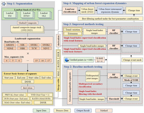
Figure 1.
The four steps of this study. RF: random forest, MAG: magnitude, DUR: duration, DSNR: disturbance signal-to-noise ratio.
- (1)
- Segmentation Preparation: We extracted and synthesized Landsat images for LandTrendr, using LandTrendr’s segmentation to obtain parameters for filtering.
- (2)
- Baseline Method Testing: We tested the accuracy of baseline methods based on extremum in identifying urban forest expansion. The two baseline methods with extremum magnitude-of-change were single-band/index filtering with threshold [15] and multispectral secondary classification [16].
- (3)
- Improved Method Testing: We tested the accuracy of improved methods with basic segment features and trend features using random forest-supervised classification.
- (4)
- Mapping of Urban Forest Expansion: We mapped the dynamics of urban forest expansion based on the method with the best accuracy.
We evaluated combinations of different maximum numbers of segments and different bands/indices to ensure that the best performance of each method is achieved.
2.1. Study Area
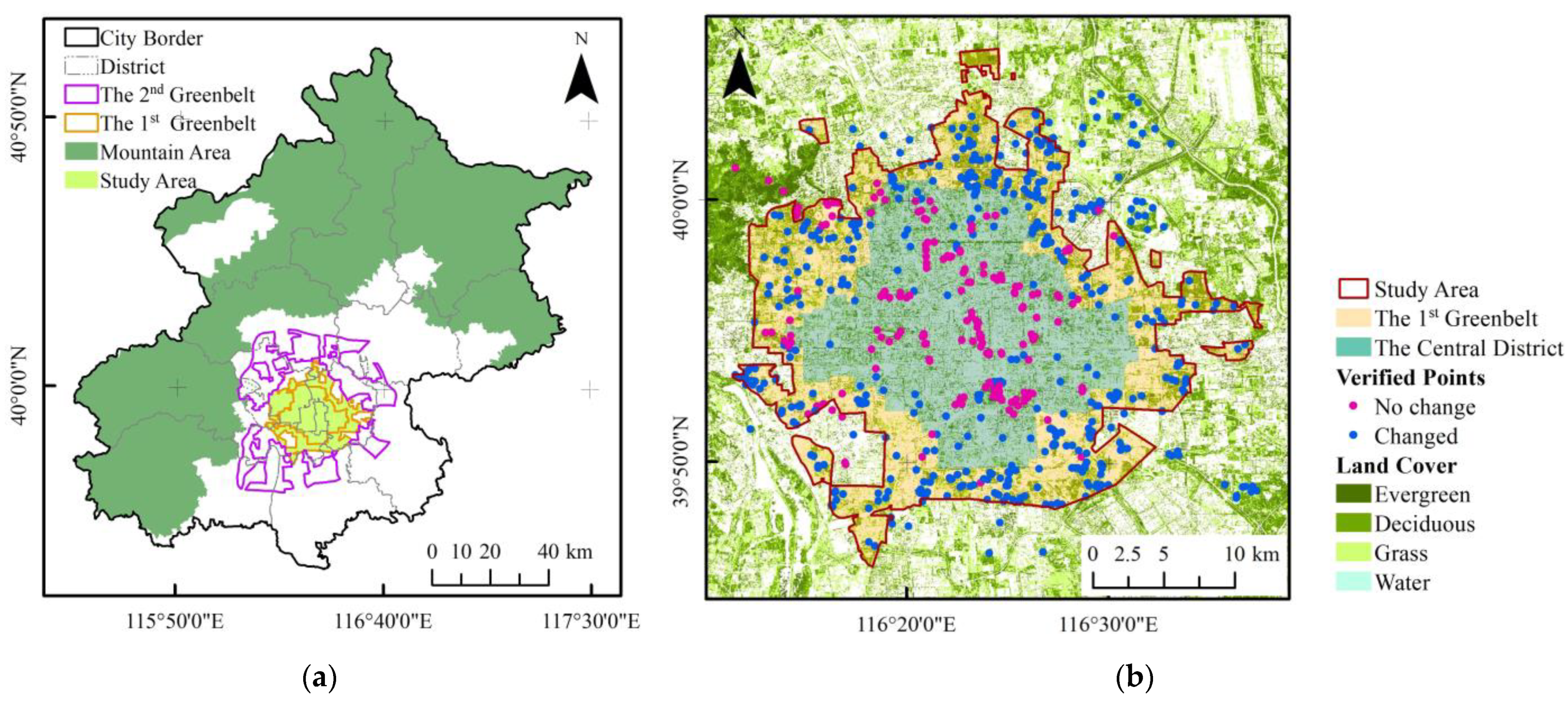
Beijing is located in the western part of the North China Plain (Figure 2a), characterized by a temperate monsoon climate with distinct seasonal vegetation features. The altitude of the plain area within the municipal boundary ranges from 20 to 60 m. The study area (Figure 2b) focuses on Beijing’s first greenbelt area (“the 1st Greenbelt”) and the Central District. This area is delineated by the outer boundary of the 1st Greenbelt, with all areas situated within the plain area. The total area is 645 km2, covering Beijing’s main built-up area and the primary scope of urban forest construction.

Figure 2.
Overview of the study area and data utilized. (a) location of the study area; (b) boundary of the study area with verified points and land cover types.
This study focuses on the urban forest construction expansion process in the study area from 1994 to 2022. The Central District is the main region of early urban construction in Beijing. To limit the ring expansion outward from the Central District, the 1st Greenbelt and the 2nd Greenbelt were planned to guide the city toward a decentralized cluster development pattern. Since 1994, Beijing has issued a series of master plans and administrative regulations to implement urban forest construction in the 1st Greenbelt [1,23], with plans to complete the 1st Greenbelt by 2035 [24]. Overall, the area bound by the outer edge of the 1st Greenbelt has been the region with the highest intensity and earliest stages of urban forest construction in Beijing to date. As the post-urbanization stage approaches, there will be an urgent need for the stock optimization of urban forests within this area.
2.2. Landsat Stack and Composite Images
Landsat Collection 2 Tier 1 Level 2 (C02/T1_L2) images were obtained and processed through the Google Earth Engine (GEE) platform, as this category of images is considered suitable for time series studies [25]. To fully capture the trends at the temporal boundaries, the image stack is a superset of the target time range (1992–2023). The annual image extraction time range is from 1 June to 30 September, as this period is Beijing’s vegetation growing season, which can fully reflect vegetation characteristics. A total of 731 available images from Landsat TM, ETM, and OLI sensors were used, including three visible bands, one near-infrared band, and two shortwave infrared bands. Clouds, snow, and shadows were removed based on the ‘QA_PIXEL’ band [25]. The bands of the images were composited into an annual representative image using the medoid composite method [26]. The medoid image is composed of the true values of the pixels closest to the median from all annual images, ensuring that the pixels typically represent the general condition.
2.3. Verified Points
The points for the actual change time used for training and validation were collected from Google Earth TM historical images of the study area and its surroundings. Based on historical image availability, the time range of the validation points was from 2001 to 2022. Three different vegetation types (evergreen vegetation, deciduous vegetation, and grass) were selected through stratified random sampling. The sample selection method involved visually inspecting all available historical images in the time series of the current sample points to determine the change time when the urban forest was constructed as of 2022. Since tree planting sometimes occurs in winter, change times after 30 September were set to the following year. Before 2001, there were fewer large-scale urban forest construction areas in Beijing, so no-change samples were fewer than changed samples. A total of 648 points were extracted (Figure 2), including 170 no-change samples and 478 changed samples. Precise coordinates, whether an urban forest was planted, and the year of change time were recorded.
To establish a stable training–evaluation process for all methods, a k-fold (k = 4) cross-validation method was used. All collected samples were divided into four training–test sets using the stratified sampling of unchanged and changed samples, ensuring that the number of unchanged and changed area sample points in each fold’s dataset was approximately equal.
2.4. LandTrendr Segmentation
Segmentation is the core step of LandTrendr [27], which groups spectral observations from Landsat annual time series stacks into a series of segments representing surface processes, achieved by removing spikes, identifying potential vertices, trajectories fitting, and simplifying [15]. To identify the optimal spectra/indices for describing the urban landcover change process and test the optimal performance, four single bands and four composite indices (Table 1) were used, namely the commonly used NBR, TCW, and NDVI in LandTrendr [15]; the high signal-to-noise ratio bands NIR, SWIR1, and SWIR2 [16]; NDMI [16,21]; and GREEN [20], which perform well in urban contexts. Composite images were processed using the LandTrendr segmentation function on the GEE platform [18]. Among all the preset parameters of LandTrendr, the maximum number of segments (max_segments) is one of the decisive parameters [15,21]. Although simple urbanization processes can summarize the spectral characteristics of land use change through three segments [10,28], the study area showed that multiple land use change processes cover the entire urbanized area. Therefore, 4–17 were selected as alternative parameters for the max_segments. Since urban forest construction is often accomplished within 1–2 years, the recovery threshold was set to 1 to accommodate one-year-long construction events [15]. In summary, 112 combinations of the max_segments and bands/indices were used for all filtering method tests.

Table 1.
Composite indices used for filtering.
2.5. Baseline Method Testing
Both baseline methods utilized the general extremum-based filtering workflow constructed on the GEE platform [18]. This program filters out the most significant disturbance events from the LandTrendr-fitted segments based on the greatest change. Urban forest construction represents a gain in vegetation, so we filtered the segments with the greatest magnitude of change within the time frame. We obtained the initial value (Preval), the year of detection (YOD), the rate of change (Rates), the magnitude of change (Mag), and the disturbance signal-to-noise ratio (DSNR) as the six feature parameters of these segments for further filtering.
2.5.1. Single-Band/Index Filtering with Threshold
Because not all greatest gains represent urban forest construction, all segments filtered by the greatest magnitude of change were further filtered by the thresholds of their basic features. We used the verified points to determine features with significant differences between changed and no-change groups using the K-S test. Then, we established a threshold grid centered on the average of the means of the two groups, divided into five intervals ranging from 0.5 to 1.5 times the group mean. Through grid search, we identified the optimal threshold combination. The greatest magnitude-of-change segments were then subjected to secondary filtering through thresholds, and the YOD of these filtered segments was used as the change time.
2.5.2. Multispectral Secondary Classification
The multispectral secondary classification is another method used to reduce the error of greatest magnitude-of-change filtering [16]. Single-band/index images with the same max_segments were combined to evaluate whether a pixel contains urban forest construction events by random forest-supervised classification. Subsequently, the change time corresponding to the urban forest construction events is derived from the mode of all images’ YOD [19].
2.6. Improved Method Testing
2.6.1. Single-Band/Index Supervised Classification
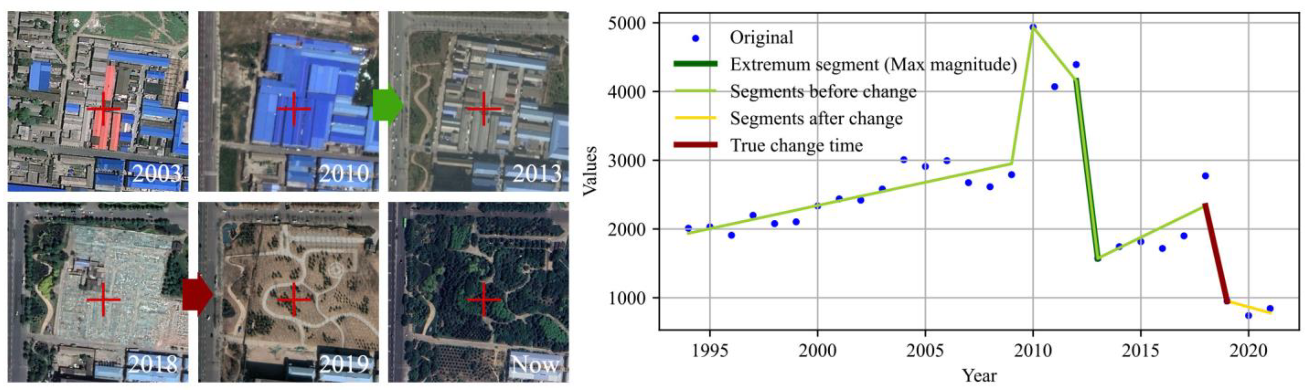
Due to the context of rapid urbanization, multiple land cover changes may occur before urban forests are planted. During this process, spectral changes often exhibit frequent and intense fluctuations. Therefore, filtering based on extreme values might mistakenly identify other land use changes as urban forest changes (Figure 3). Due to temporary vegetation during the land preparation process and sparse planting at the beginning of construction, the spectral characteristics at the time of urban forest establishment may not be distinct, potentially causing further difficulties in filtering.

Figure 3.
An example of the land cover changes keyframes with the corresponding segments fitted by LandTrendr under the SWIR2. The red cross in keyframes represents the sample point processed by the LandTrendr, the green arrow indicates the process extracted by the greatest magnitude of change, and the dark red arrow shows the actual urban forest construction event.
To reduce the potential errors caused by extremum filtering, the improved method employed supervised classification to identify the common characteristics of segments representing urban forest construction events. After segmentation, all segments in the time series and their features describing each segment were retained. These features included magnitude, rates, start value, end value, start year, end year, duration, and DSNR (Figure 1). The images with multiple segments were processed on the GEE platform [18] and then saved offline for further processing. The construction of subsequent filtering methods improvement was carried out in Python 3.9.
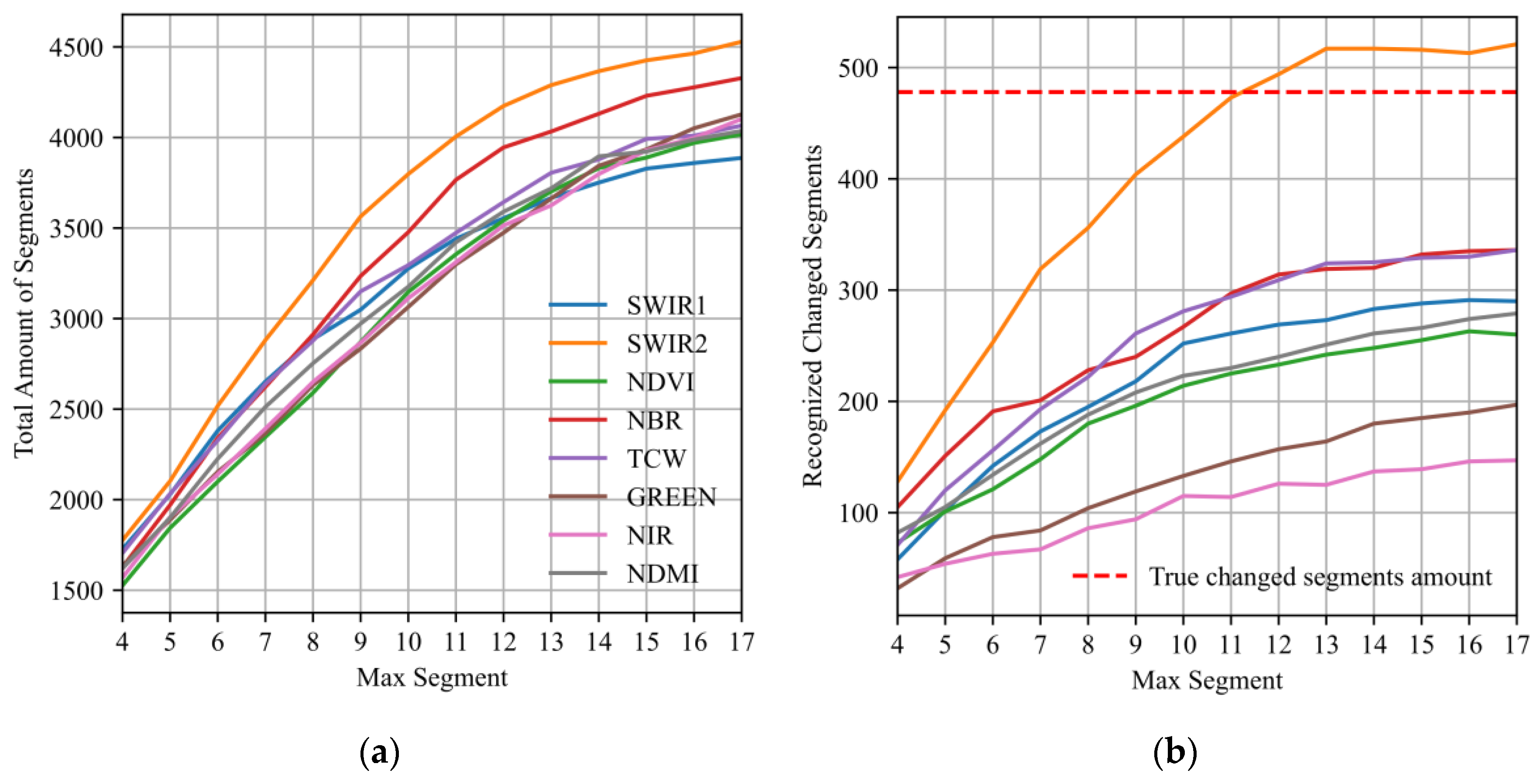
To construct a training–test set for supervised classification, segments representing true urban forest construction events were identified based on the matching of true change times from verified points and the end-year features of the segments. Segments identified as construction events and other segments were categorized into two subsets: changed and no change (Figure 4).

Figure 4.
Segment identification results at all preset parameter combinations: (a) amount of all segments fitted by LandTrendr from the training and validation sets; (b) amount of the identified changed segments from the training and validation sets.
The random forest classifier uses an ensemble of decision trees to make reliable predictions [33], which is particularly advantageous in handling high-dimensional data, as it can automatically select and rank the most relevant features [34]. Random forest was run on all folds of the training set via a hyperparametric grid containing n_estimator (100, 200, 500), max_depth (None, 10, 20, 30), max_samples_split (2, 5, 10), and max_samples_leaf (1, 2, 4). Since the no-change segments vastly outnumber the changed segments, Balanced_class_weight was applied to address this imbalance of changed and no-change segments in the training samples. Next, sample points where urban forest construction events happened were filtered from all samples by the changed mask obtained using the multispectral secondary classification method. The optimal hyperparameter combination with the average optimal result overall folds of the test set was used as the final result to characterize the performance of the improved method.
2.6.2. Single-Band/Index Supervised Classification with Trend Features
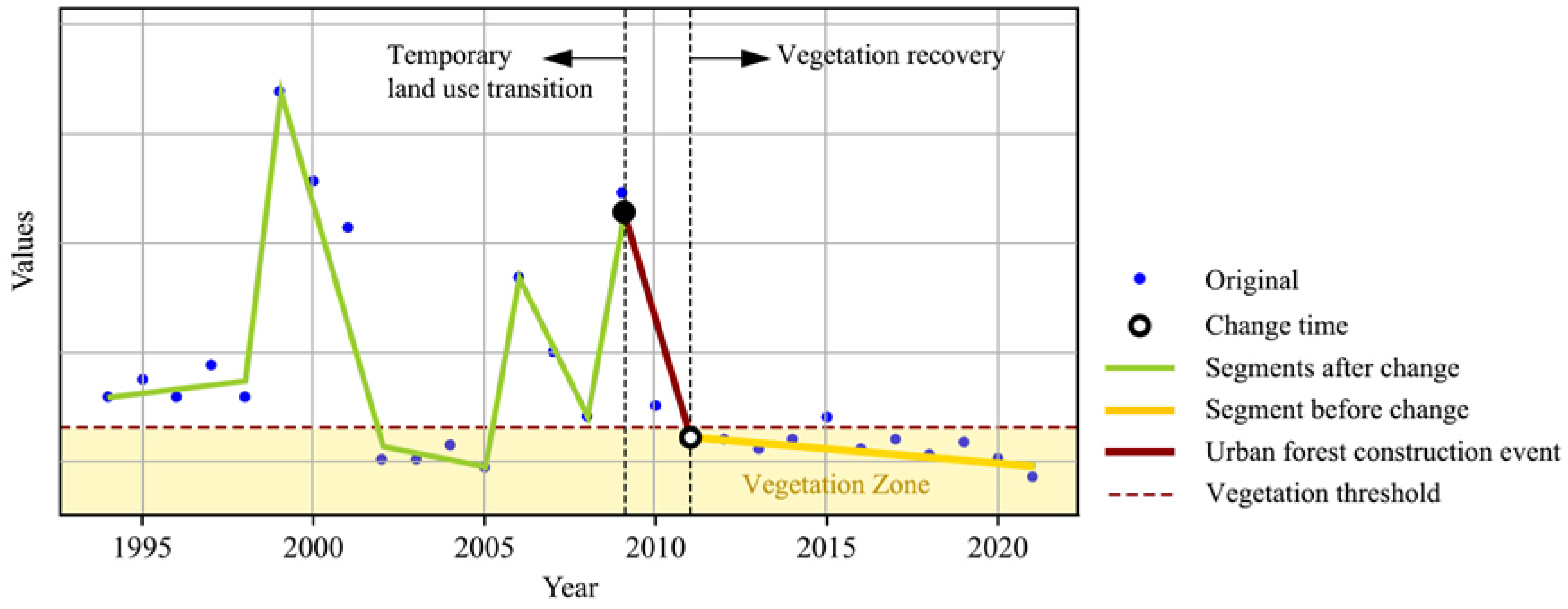
The specific spectral change patterns of urban forests provide guidance for identifying the exact change time of land cover (Figure 5). Regarding the amplitude of spectral fluctuations, the surface spectra typically maintain a stable trend after construction, indicating the growth process of vegetation after planting. Conversely, urban planning and development before urban forest construction can cause fluctuations in spectral values. Numerically, the transition from non-vegetated to vegetated areas before and after urban forest construction results in a significant contrast in spectral values.
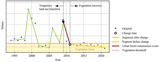
Figure 5.
Urban land use transition pattern in urban forest construction areas (using the segmentation results of the SWIR2 band as an example).
Therefore, extracting the mean values of each spectral fitting segment, which represents urban land use patterns, helps to determine whether a transition from non-vegetated to vegetated areas has occurred before and after the segment (Equations (1) and (2)).
where is the basic feature to be quantized, which can be rates, magnitude, durations, start values, and end values; is the index of the target segment; is the total number of segments; is the average of for all segments before segment ; and is the average of the for all segments after segment .
By extracting the standard deviation to capture the fluctuations in land use patterns before and after each segment, it is possible to identify whether the process represented by the segment leads to a stable spectral state indicative of stable vegetation growth (Equations (3) and (4)).
where is the standard deviation of for all segments before segment , and is the standard deviation of for all segments after segment . When segment is the second/penultimate segment, the features of segment 1/ are used for virtual extension. When segment is the last/first segment, its / is set to 0.
In addition to the above-added feature variables and all the basic features, we also set a batch of categorical variables by whether they were the overall maximum/minimum value and their ranking in the time series.
The improvement with trend features used exactly the same steps in training set construction and model training as the improved method with basic features. A total of 88 variables (Table A1) were screened by feature importance tests at two time points, and 38 feature variables were used for the final filtering test (Table 2).
Table 2.
Features used for the improved method with trend features.
2.7. Evaluation of the Filtering Performance
The filtering performance of all methods was comprehensively evaluated in two dimensions: whether the change could be identified and whether the change time could be accurately extracted.
In one-fold data, due to the imbalance of no-change and changed samples, the ability to accurately predict urban forest change was evaluated using the area under the ROC curve (AUC) [35]. When AUC equals 1, it indicates that the algorithm can completely distinguish between no-change and changed samples.
For the identification of change time, we used accuracy instead of a continuous-variable approach (Equation (5)). For the reasons mentioned in Section 2.3, a predicted change time that differs from the true change time by ±1 year was considered accurate.
where TP represents the sample in which the extracted change time difference is less than or equal to 1 year, and TN represents the areas identified as unchanged. FP represents the areas identified as changed but actually unchanged, and FN represents the areas identified as unchanged but actually changed.
The overall performance of each method was determined with the mean and standard deviation of all folds to reduce the potential test errors caused by sample selection.
2.8. Urban Forest Mask and Expansion Dynamic Mapping
The change time of urban forests identified by the best-performing method was used to create an expansion dynamic map of urban forests. An urban forest mask was used to limit the identified areas to the urban forest range, thereby reducing interference from other land use types. We defined all vegetation within the study area as urban forest, including evergreen vegetation, deciduous vegetation, and grass. In the rapid urbanization process, there is a phenomenon of vegetation being temporarily removed and then re-vegetated. To avoid confusing this situation with unchanged vegetation, a static urban forest mask was only extracted in 2022. Pixel-level land cover classification for the 2022 Landsat medoid composite image was achieved using random forest-supervised classification [36], categorizing the land cover into grass, evergreen trees, deciduous trees, water bodies, and impervious surfaces, with an overall accuracy of 0.85 (Table A2). Eight-neighborhood mode filtering was used to eliminate the effect of salt-and-pepper noise from isolated change pixels in the mapping results.
3. Results
3.1. Filtering Performance of the Baseline Methods
The performance of the single-band/index filtering with threshold varied considerably across different bands/indices (Figure 6). Most of the bands/indices had an AUC of between 0.5 and 0.75 in recognizing change events. In terms of the change time, more than half of the samples in the test predicted the wrong time of change. The spectral type of best performance was SWIR2, which had an average accuracy of 51.40 ± 0.05% for the change time when the max_segments was 14.
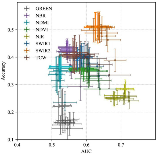
Figure 6.
Average performance and standard deviation of the single-band/index filtering with thresholds in identifying change events and their timings. The higher brightness indicates a higher max_segments.
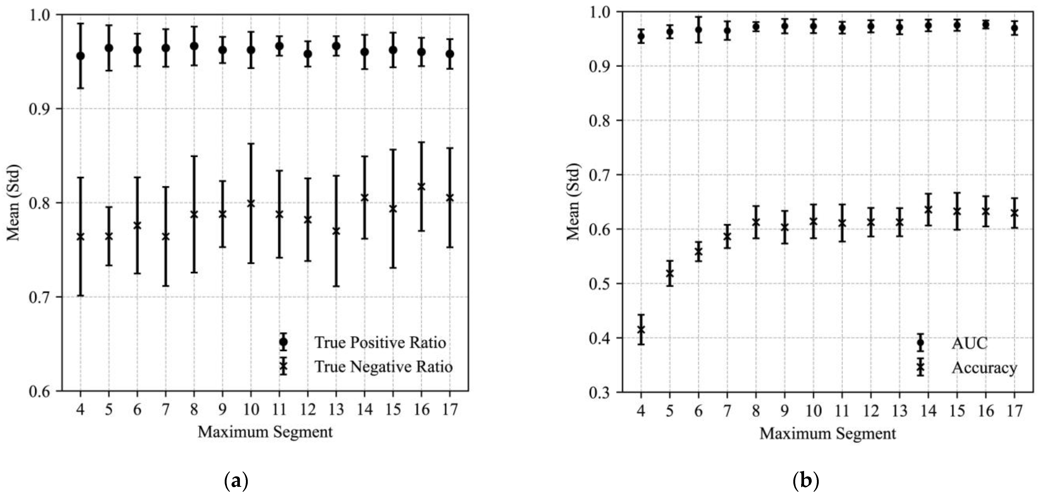
In the multispectral secondary classification, as the max_segments increased, the number of true positives in identifying change time slightly decreased, while the number of true negatives slightly increased (Figure 7a), but the ability to identify unchanged samples was relatively weak. Almost all max_segments scenarios showed stable and excellent performance in identifying construction events (Figure 7b), indicating a strong ability to distinguish no-change and changed areas, with the highest AUC being 0.98 ± 0.01 (max_segments = 16). In terms of identifying change time, the performance was generally weak.

Figure 7.
Performance evaluation of the multispectral secondary classification in identifying change events and timings: (a) the ratio of true positives and true negatives in identifying construction events; (b) the AUC in identifying construction events and the accuracy in identifying change time.
According to the feature importance evaluation of multispectral secondary classification, the trend of feature importance was generally consistent across different maximum numbers of segments in identifying construction events (Figure A1). In the extraction of change time by secondary classification, PREVAL and magnitude were the most important features. The PREVAL and magnitude from SWIR2 were the two most important predictive variables.
3.2. Filtering Performance of the Improved Methods
The improved method with basic features outperformed all baseline methods in identifying change time (Figure 8a). The best parameter combination (SWIR2, max_segments = 13) achieved a mean accuracy of 71.30 ± 4.59%. The improved method with trend features performed even better (Figure 8b), achieving the highest mean accuracy of 89.35 ± 4.96% with the same best parameter combination.
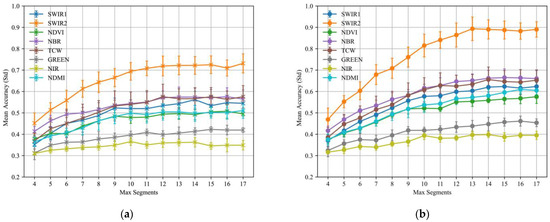
Figure 8.
Accuracy of identifying change time for all parameter combinations using the improved method based on single spectral supervised classification: (a) accuracy of the improved method based on basic features; (b) accuracy of the improved method based on relative trend features.
Similar to the baseline methods, SWIR2 had the highest performance. Other bands/indices performed no better than multispectral secondary classification in evaluating change time. As the max_segments increased, the accuracy of identifying change time grew steadily and then stabilized.
The improved method with basic features exhibited an increase in (Table 3) the true-positive rate (78.92 ± 3.48%) in identifying change times but still did not yield a sufficient true-negative rate in detecting unchanged areas (60.57 ± 6.69%).
Table 3.
The performance of the improved method with basic features and optimal parameter combination (SWIR2, max_segments = 13).
The improved method with trends achieved higher accuracy in identifying both changed and unchanged areas (Table 4), performing better than the improved method with basic features. Notably, the accuracy in identifying changed areas (90.12 ± 5.65%) was slightly higher than in identifying unchanged areas (87.40 ± 5.95%).
Table 4.
The performance of the improved method with trend features and optimal parameter combination (SWIR2, max_segments = 13).
According to the feature importance evaluation of two improved methods, the rate consistently emerged as the most important feature. In the improved method with basic features, magnitude was the second important feature, followed by DSNR, start value, end value, and duration.
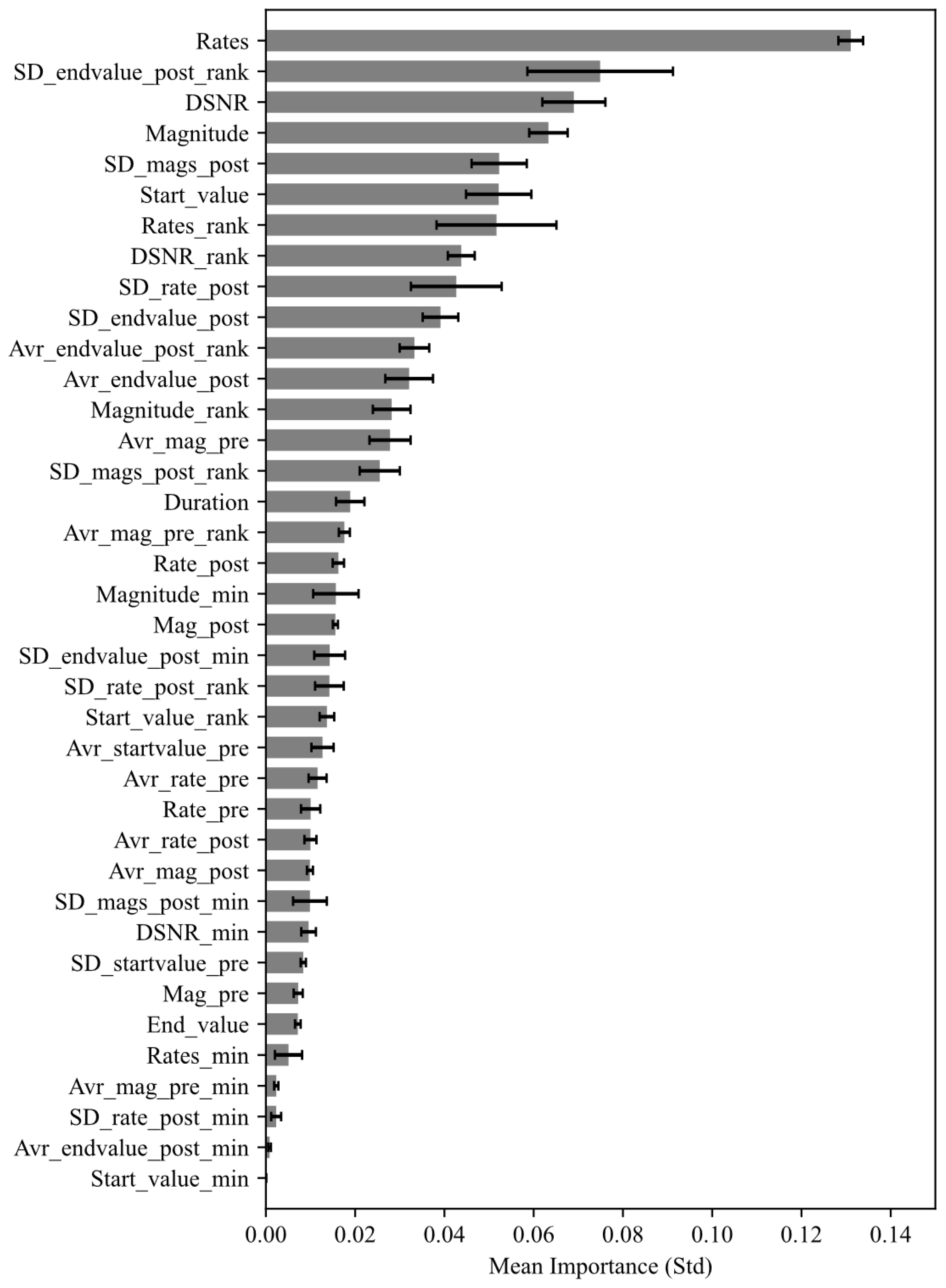
As for the feature importance of the improved method with trend features (Figure 9), post-change-trend features played an important role in the identification. Although the maximum value features of rate and magnitude are the primary features in traditional extremum-based methods, their impact on identifying urban forest construction events is negligible (Table A1), whereas the minimum value and ranking features proved valuable in the change time identification.
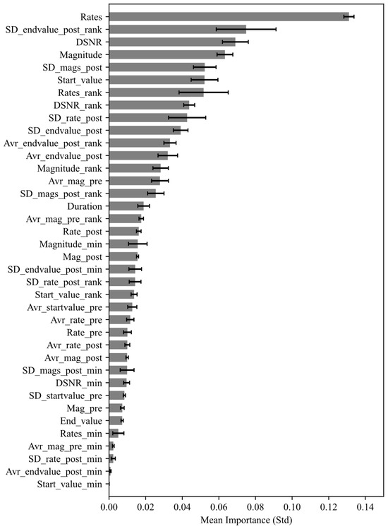
Figure 9.
The mean and standard deviation of feature importance under different combinations of preset parameters and bands/indices in the improved method with trend features.
3.3. The Expansion Dynamic Mapping of Urban Forests in the Study Area
Using the improved method with trend features under the optimal parameter combination, an urban forest expansion dynamic map was established (Figure 10a). In terms of expansion in the study area, the urban forest area existing before 1994 was 96.26 km2, with an additional urban forest area of 141.35 km2 until 2022.
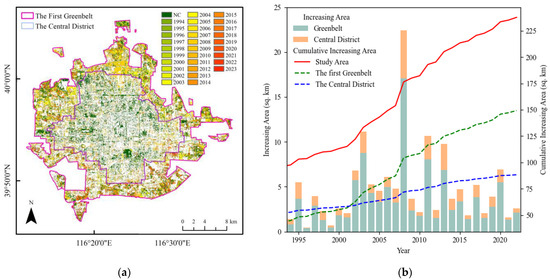
Figure 10.
(a) Urban forest dynamic map of the study area; (b) annual and cumulative increase in urban forest area in the study area.
Based on the urban forest expansion process (Table 5), the urban forest of the study area increased to 22.26% in the urban forest coverage rate during the rapid expansion period. The most significant growth occurred in the 1st Greenbelt, where urban forest expanded by 3.38 times. In contrast, the urban forest in the Central District expanded by less than twice.
Table 5.
Comparison of urban forest expansion processes across different regions within the study area.
Based on the annual statistics of newly constructed urban forest areas, the growth rate of urban forests shows an unstable pattern (Figure 10b). The years 2003, 2008, 2011, 2013, and 2020 were notable for increases relative to the overall expansion trend, while in other years, the expansion trend was uneven. Combining the Beijing urban forest construction promotion policies released in 2000, 2008, and 2012, it is clear that after the release of incentive policies for green space construction, the intensity of urban forest construction increased significantly. The most notable increase was in 2008, coinciding with the Beijing Summer Olympics, which led to the dramatic urban forest expansion of the 1st Greenbelt.
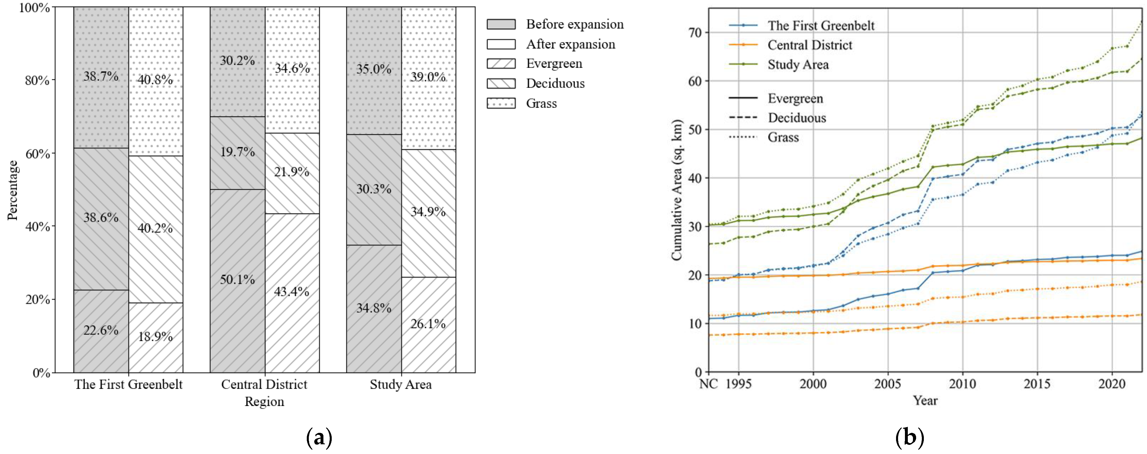
Based on the distribution of vegetation types before and after urban forest expansion (Figure 11a). The urban forest construction process from 1994 to 2022 altered the composition of vegetation types in the urban forest of this area. The dominant type gradually shifted from evergreen vegetation to deciduous vegetation, primarily driven by the construction of the greenbelt. Considering the function types of urban forests in Beijing, the main vegetation was concentrated in royal gardens and modern parks before 1994, with evergreen trees contributing to the solemn atmosphere of the ancient capital. As Beijing’s urban forest development gradually shifted toward public greenspace focused on ecological and recreational benefits, the proportion of deciduous trees and grasslands increased.
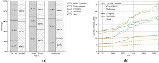
Figure 11.
Expansion of vegetation types in the Central District and the 1st Greenbelt: (a) the distributions of vegetation type before and after expansion; (b) expansion process during the expansion process.
Based on the dynamics of vegetation type development (Figure 11b), due to the clear designation and rapid development of the 1st Greenbelt around 2002, the rapid increase in the growth rate of deciduous trees caused their total number to surpass that of evergreen trees within the study area. After 2008, the growth rate of grasslands gradually accelerated, mainly due to the slowing growth rate of deciduous trees in the 1st Greenbelt. According to Beijing’s urban forest construction policies, with a significant increase in greenery, the overall progress of greenspace construction shifted to fine-scale construction with villages and towns as implementation units. Our study indicates that this phase of urban forest expansion reduced the supply of trees. The central area did not show significant growth inflection points during this period, maintaining a relatively stable development trend.
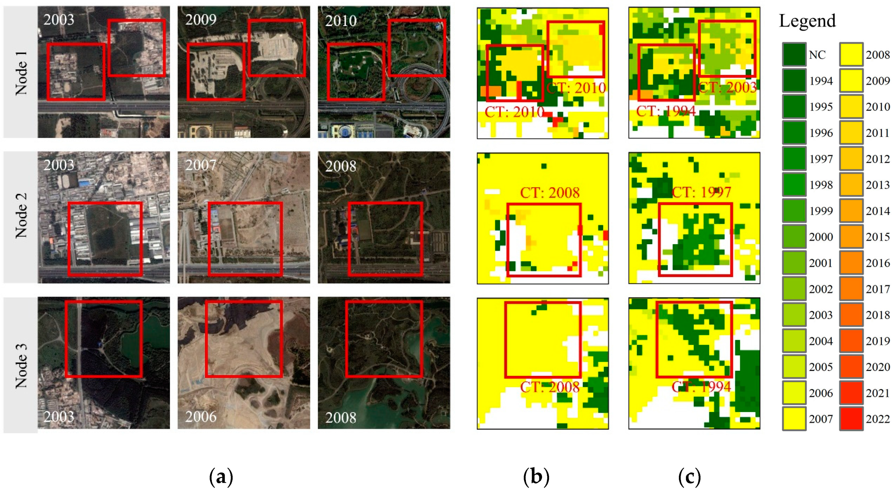
Three examples outside the validation point areas were used to demonstrate the accuracy improvement in expansion dynamic mapping (Figure 12). Baseline methods (Figure 12c) tended to overlook the disturbance and recovery processes of urban forests, leading to the overestimation of the duration of urban forest presence. The improved method (Figure 12b), by capturing vegetation renewal trends, could more accurately determine the current planting time of vegetation.
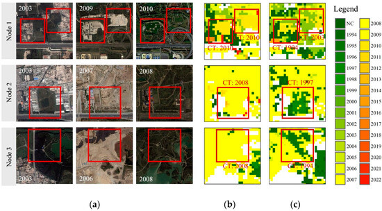
Figure 12.
Examples of change time map comparison between the multispectral secondary classification method and the improved method with trend features. Areas in red boxes are areas with differential identification results. CT: change time, NC: no change: (a) keyframe Google Earth TM historical image of the areas over the time series; (b) change time maps based on the improved method with trend features; (c) change time maps based on the baseline method of multispectral secondary classification.
4. Discussion
4.1. Characteristics of the Improved Methods
Although there have been attempts at filtering by exploiting the role of high-dimensional information provided by LandTrendr [17,20], no specific study has focused on urban forests or single-event identification. Compared to the single-band/index baseline method, the improved method with trend features improved the accuracy by 38%, while it improved the accuracy by 25% compared to the multispectral secondary classification.
In order to test the reusability of the improved method with trend features in different areas, the optimal model selected during testing with the best parameter combination was used to identify the expansion of urban forest in the 2nd Greenbelt (Figure 2a). As the results of the 162 verified samples indicate, the accuracy of the improved method with trend features reached 88.27%, suggesting that the method performed satisfactorily in other regions as well.
The improved methods were able to avoid the errors caused by the data downscaling of extremum segment filtering, thus revealing the characteristics of urban forest construction events over the entire land use life cycle through higher dimensional quantity and trend relationships. The performance of urban forest construction event filtering can be improved by adding targeted features [27]. According to the feature importance assessment, each basic feature was in an important position in the improved methods. This indicates that relative to the extreme-value features, feature quantities are significant in distinguishing urban forests. Trend features played an auxiliary role in improving the identification of urban forests, in which the main features were the trend after change. The global extreme value played a very small role in the filtering, indicating the limitation of the maximum value based on the magnitude of change in identifying urban forest growth. We also assessed urban forest construction events that were not accurately filtered. The improved methods may still have difficulty in identifying the areas in which the change time was close to the time boundary due to underfitting.
4.2. Bands/Indices and Parameter Optimization for Urban Forest Detection
According to the results of optimal parameter combinations, SWIR2 was more effective than other bands/indices because SWIR2 tended to retain more detailed segments of changes (Figure 4). Although this may lead to information redundancy, it provides more opportunities for further filtering. Based on the analysis by Cohen et al. [16], SWIR and NIR, along with their composite indices, exhibit the highest efficiency. However, in our testing, NIR’s performance was not as prominent as that of the SWIR2 band. This is likely due to the relatively low initial vegetation density in urban forests, with SWIR2 being more sensitive to sparse vegetation areas [27].
On the other hand, appropriately increasing the maximum number of segments can enhance filtering performance. In the baseline methods, with a lower maximum number of segments, we could accurately identify construction events in the area but failed to extract the precise change time, indicating that LandTrendr segmentation led to the loss of change details. However, when the maximum number of segments covered the total number of events, the LandTrendr algorithm did not continue to add details to the fitted graph (Figure 4). Given the characteristics of the preset parameters, retaining as much change detail as possible during the segmentation process can improve identification effectiveness when recognizing land use changes under rapid urbanization. Additionally, we reiterate that adjusting the recovery threshold is necessary to address rapid urbanization cycles [19,21], as most detected urban forest construction events occur within 1–2 years.
4.3. Annual Dynamics Benefit Urban Forest Management
Annual urban forest expansion dynamics can reveal the details of the expansion process and provide a clear understanding of how these changes occur throughout the urban development process. Combining semantic information, such as vegetation types or greenspace types, can provide trend insights for optimizing the management of urban forests. Considering the study area, there have been many assessments of Beijing’s urban forest development [11,37]. However, the method of 5-year cross-section comparison can only determine potential driving factors and overall trends [38,39], making it difficult to identify the specific impacts of policies on vegetation expansion. By analyzing annual spatial dynamics, urban forest promotion events can be correlated with specific construction processes over time [22], significantly enhancing the interaction feedback process between policies and construction activities.
On the other hand, urban forest expansion dynamic detection promotes urban vegetation renewal. Change time identification can represent the age of vegetation relative to planting, which is related to the ecological benefits of vegetation [40,41]. Remote sensing-based dynamic identification can reduce the workload of on-site vegetation surveys. The assessment of the overall spatial distribution allows for the scientific formulation of a gradual renewal implementation path across the city. Enhancing identification accuracy can avoid additional costs caused by data errors in digital urban forest management.
4.4. Limitations
One of the main problems with using Landsat for urban forest identification is the relatively low image resolution. However, given the cost and the availability of time series images over a time span of more than twenty years, the loss of resolution is acceptable.
The improved method was implemented in the context of rapid urbanization in Beijing. Although China’s rapid urbanization development process has been characterized by relatively consistent changes over the past 40 years or so [2], the applicability of the proposed method for identifying the characteristics of china and the global urbanization process still requires further validation. Another issue is the implementation efficiency. Although the algorithm has an efficiency advantage over cross-sectional classification and comparison, its efficiency is reduced due to steps such as preparation for supervised classification and cross-platform data transfer, compared to the well-established extremum-based filtering workflow on GEE. However, since previous filtering methods lack the ability to improve accuracy in recognizing change times, improving the method is still of clear value at this time.
5. Conclusions
Our study integrates the trend features of urban surface dynamics into the identification of urban forest expansion using random forest classification, establishing a filtering method based on single spectral features. By identifying the spectral quantity and fluctuation characteristics before and after urban forest construction, the accuracy of LandTrendr in detecting urban forest expansion was significantly improved. Compared to baseline methods, the accuracy of the improved method increased by over 25%. Validating the reliability of this method in different land use change scenarios and integrating the workflow with GEE’s cloud computing process are the primary directions for future development.
Accurate urban forest expansion dynamics enable detailed post-implementation assessments of urban forest initiatives, promote quantitative research on process mechanisms, and significantly advance the scientific evaluation and renewal strategies of urban forests.
Author Contributions
Conceptualization, Z.L.; methodology, Z.L.; software, Z.L. and Y.Z.; validation, Z.L.; formal analysis, Z.L.; investigation, Z.L. and Y.Z.; resources, Z.L. and X.Z.; data curation, Z.L.; writing—original draft preparation, Z.L. and Y.Z.; writing—review and editing, Z.L. and Y.Z.; visualization, Z.L.; supervision, Z.L. and X.Z.; project administration, Z.L. and X.Z.; funding acquisition, X.Z. All authors have read and agreed to the published version of the manuscript.
Funding
This research was funded by the National Natural Science Foundation of China, grant number 32371643.
Data Availability Statement
The data presented in this study are available upon request from the corresponding author.
Conflicts of Interest
The authors declare no conflicts of interest.
Appendix A
Table A1.
Segment features for implementing the improved method classification and selected results.
Table A1.
Segment features for implementing the improved method classification and selected results.
| Ranking | Name | Feature Importance | Selected Features |
|---|---|---|---|
| 1 | Rates | 0.1265 | ✓ |
| 2 | DSNR | 0.0647 | ✓ |
| 3 | Magnitude | 0.0564 | ✓ |
| 4 | SD_endvalue_post_rank | 0.056 | ✓ |
| 5 | Rates_rank | 0.0467 | ✓ |
| 6 | SD_endvalue_post | 0.0419 | ✓ |
| 7 | SD_rate_post | 0.0383 | ✓ |
| 8 | Start_value | 0.0373 | ✓ |
| 9 | Avr_mag_pre | 0.0314 | ✓ |
| 10 | SD_mags_post_rank | 0.031 | ✓ |
| 11 | Avr_endvalue_post_rank | 0.0306 | ✓ |
| 12 | SD_mags_post | 0.0291 | ✓ |
| 13 | DSNR_rank | 0.0284 | ✓ |
| 14 | Magnitude_rank | 0.0252 | ✓ |
| 15 | Avr_endvalue_post | 0.0209 | ✓ |
| 16 | SD_rate_post_rank | 0.0192 | ✓ |
| 17 | Avr_mag_pre_rank | 0.0186 | ✓ |
| 18 | Start_value_rank | 0.0156 | ✓ |
| 19 | Duration | 0.0154 | ✓ |
| 20 | DSNR_min | 0.0131 | ✓ |
| 21 | SD_mags_post_min | 0.0129 | ✓ |
| 22 | Mag_post | 0.0129 | ✓ |
| 23 | Rate_post | 0.0126 | ✓ |
| 24 | Rates_min | 0.0124 | ✓ |
| 25 | Magnitude_min | 0.0103 | ✓ |
| 26 | Avr_rate_pre | 0.0099 | ✓ |
| 27 | SD_rate_post_min | 0.0097 | ✓ |
| 28 | Avr_rate_pre_rank | 0.0095 | |
| 29 | Avr_startvalue_pre | 0.0092 | ✓ |
| 30 | Mag_pre | 0.009 | ✓ |
| 31 | Start_value_max | 0.0085 | |
| 32 | SD_endvalue_post_min | 0.0084 | ✓ |
| 33 | Rate_pre | 0.0076 | ✓ |
| 34 | Avr_startvalue_pre_rank | 0.0072 | |
| 35 | SD_startvalue_pre | 0.0067 | |
| 36 | Avr_rate_post | 0.0063 | ✓ |
| 37 | Rate_post_rank | 0.0061 | |
| 38 | Avr_mag_post | 0.0061 | ✓ |
| 39 | End_value | 0.006 | ✓ |
| 40 | SD_rate_pre | 0.0057 | |
| 41 | SD_mags_pre | 0.0053 | |
| 42 | Mag_pre_rank | 0.0049 | |
| 43 | Mag_post_rank | 0.0049 | |
| 44 | Rate_pre_rank | 0.0045 | |
| 45 | Avr_rate_post_rank | 0.0044 | |
| 46 | Avr_mag_post_rank | 0.0044 | |
| 47 | SD_startvalue_pre_rank | 0.0043 | |
| 48 | SD_rate_pre_rank | 0.0034 | |
| 49 | SD_mags_pre_rank | 0.003 | |
| 50 | Avr_mag_pre_min | 0.003 | ✓ |
| 51 | Duration_rank | 0.003 | |
| 52 | End_value_rank | 0.0028 | |
| 53 | Avr_rate_post_min | 0.0026 | |
| 54 | Avr_mag_post_min | 0.0021 | |
| 55 | Avr_mag_pre_max | 0.002 | |
| 56 | Rate_post_min | 0.0019 | |
| 57 | Duration_max | 0.0017 | |
| 58 | Duration_min | 0.0017 | |
| 59 | Avr_endvalue_post_min | 0.0016 | ✓ |
| 60 | SD_startvalue_pre_min | 0.0015 | |
| 61 | End_value_max | 0.0014 | |
| 62 | Avr_rate_pre_max | 0.001 | |
| 63 | SD_rate_pre_min | 0.0008 | |
| 64 | Avr_rate_pre_min | 0.0008 | |
| 65 | SD_mags_pre_min | 0.0007 | |
| 66 | SD_mags_pre_max | 0.0006 | |
| 67 | SD_startvalue_pre_max | 0.0006 | |
| 68 | Mag_post_min | 0.0006 | |
| 69 | SD_endvalue_post_max | 0.0006 | |
| 70 | Mag_pre_max | 0.0005 | |
| 71 | End_value_min | 0.0005 | |
| 72 | Rate_pre_min | 0.0005 | |
| 73 | Avr_startvalue_pre_min | 0.0005 | |
| 74 | Rate_pre_max | 0.0005 | |
| 75 | DSNR_max | 0.0005 | |
| 76 | Avr_startvalue_pre_max | 0.0005 | |
| 77 | Avr_rate_post_max | 0.0004 | |
| 78 | SD_mags_post_max | 0.0004 | |
| 79 | Mag_post_max | 0.0003 | |
| 80 | Mag_pre_min | 0.0003 | |
| 81 | Avr_mag_post_max | 0.0003 | |
| 82 | Rate_post_max | 0.0003 | |
| 83 | SD_rate_post_max | 0.0003 | |
| 84 | SD_rate_pre_max | 0.0003 | |
| 85 | Rates_max | 0.0002 | |
| 86 | Start_value_min | 0.0002 | ✓ |
| 87 | Avr_endvalue_post_max | 0.0001 | |
| 88 | Magnitude_max | 0 |
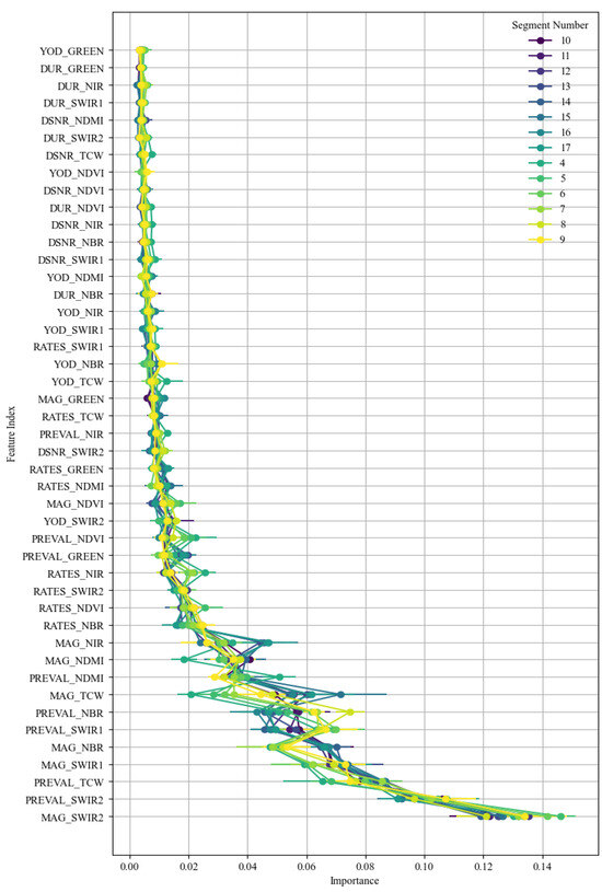
Figure A1.
Feature importance of the secondary classification.
Figure A1.
Feature importance of the secondary classification.
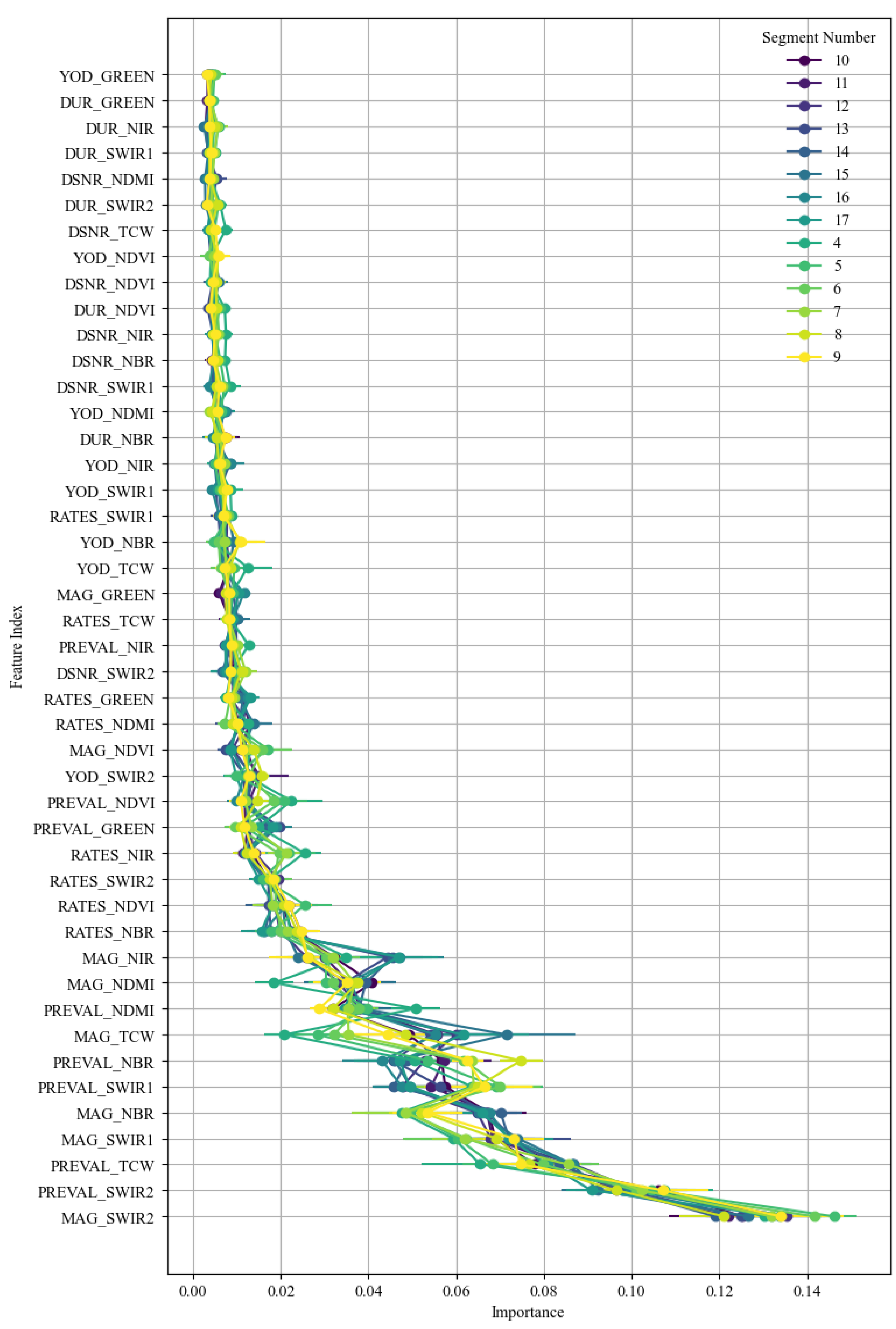
Table A2.
Classification accuracy of the urban forest mask.
Table A2.
Classification accuracy of the urban forest mask.
| Real Value Projected Value | Evergreen Trees | Deciduous Trees | Grass | Water Bodies | Impervious Surfaces |
|---|---|---|---|---|---|
| Evergreen trees | 65 | 14 | 2 | 1 | 0 |
| Deciduous trees | 5 | 48 | 9 | 2 | 0 |
| Grassland | 7 | 3 | 54 | 1 | 0 |
| Water bodies | 2 | 1 | 0 | 80 | 1 |
| Impervious surfaces | 0 | 0 | 4 | 2 | 64 |
| Producer accuracy (PA) | 0.79 | 0.75 | 0.83 | 0.95 | 0.91 |
| User accuracy (UA) | 0.82 | 0.73 | 0.78 | 0.93 | 0.98 |
| Overall accuracy (OA) | 0.85 | ||||
| Kappa index | 0.81 | ||||
References
- Yao, N.; Konijnendijk van den Bosch, C.C.; Yang, J.; Devisscher, T.; Wirtz, Z.; Jia, L.; Duan, J.; Ma, L. Beijing’s 50 Million New Urban Trees: Strategic Governance for Large-Scale Urban Afforestation. Urban For. Urban Green. 2019, 44, 126392. [Google Scholar] [CrossRef]
- Sun, L.; Chen, J.; Li, Q.; Huang, D. Dramatic Uneven Urbanization of Large Cities throughout the World in Recent Decades. Nat. Commun. 2020, 11, 5366. [Google Scholar] [CrossRef] [PubMed]
- Cadaval, S.; Clarke, M.; Roman, L.A.; Conway, T.M.; Koeser, A.K.; Eisenman, T.S. Managing Urban Trees through Storms in Three United States Cities. Landsc. Urban Plan. 2024, 248, 105102. [Google Scholar] [CrossRef]
- Shen, G.; Wang, Z.; Liu, C.; Han, Y. Mapping Aboveground Biomass and Carbon in Shanghai’s Urban Forest Using Landsat ETM+ and Inventory Data. Urban For. Urban Green. 2020, 51, 126655. [Google Scholar] [CrossRef]
- Zhuang, Q.; Shao, Z.; Gong, J.; Li, D.; Huang, X.; Zhang, Y.; Xu, X.; Dang, C.; Chen, J.; Altan, O.; et al. Modeling Carbon Storage in Urban Vegetation: Progress, Challenges, and Opportunities. Int. J. Appl. Earth Obs. Geoinf. 2022, 114, 103058. [Google Scholar] [CrossRef]
- Lin, J.; Kroll, C.N.; Nowak, D.J.; Greenfield, E.J. A Review of Urban Forest Modeling: Implications for Management and Future Research. Urban For. Urban Green. 2019, 43, 126366. [Google Scholar] [CrossRef]
- Hilbert, D.R.; Roman, L.A.; Koeser, A.K.; Vogt, J.; Doorn, N.S. Urban Tree Mortality: A Literature Review. Arboric. Urban For. 2019, 45, 167–200. [Google Scholar] [CrossRef]
- Wang, J.; Zhou, W.; Qian, Y.; Li, W.; Han, L. Quantifying and Characterizing the Dynamics of Urban Greenspace at the Patch Level: A New Approach Using Object-Based Image Analysis. Remote Sens. Environ. 2018, 204, 94–108. [Google Scholar] [CrossRef]
- Chen, W.; Huang, H.; Dong, J.; Zhang, Y.; Tian, Y.; Yang, Z. Social Functional Mapping of Urban Green Space Using Remote Sensing and Social Sensing Data. ISPRS J. Photogramm. Remote Sens. 2018, 146, 436–452. [Google Scholar] [CrossRef]
- Yang, Z.; Fang, C.; Li, G.; Mu, X. Integrating Multiple Semantics Data to Assess the Dynamic Change of Urban Green Space in Beijing, China. Int. J. Appl. Earth Obs. Geoinf. 2021, 103, 102479. [Google Scholar] [CrossRef]
- Yang, J.; Jinxing, Z. The Failure and Success of Greenbelt Program in Beijing. Urban For. Urban Green. 2007, 6, 287–296. [Google Scholar] [CrossRef]
- Zhu, Z. Change Detection Using Landsat Time Series: A Review of Frequencies, Preprocessing, Algorithms, and Applications. ISPRS J. Photogramm. Remote Sens. 2017, 130, 370–384. [Google Scholar] [CrossRef]
- Zhu, Z.; Woodcock, C.E.; Olofsson, P. Continuous Monitoring of Forest Disturbance Using All Available Landsat Imagery. Remote Sens. Environ. 2012, 122, 75–91. [Google Scholar] [CrossRef]
- Verbesselt, J.; Zeileis, A.; Herold, M. Near Real-Time Disturbance Detection Using Satellite Image Time Series. Remote Sens. Environ. 2012, 123, 98–108. [Google Scholar] [CrossRef]
- Kennedy, R.E.; Yang, Z.; Cohen, W.B. Detecting Trends in Forest Disturbance and Recovery Using Yearly Landsat Time Series: 1. LandTrendr—Temporal Segmentation Algorithms. Remote Sens. Environ. 2010, 114, 2897–2910. [Google Scholar] [CrossRef]
- Cohen, W.B.; Yang, Z.; Healey, S.P.; Kennedy, R.E.; Gorelick, N. A LandTrendr Multispectral Ensemble for Forest Disturbance Detection. Remote Sens. Environ. 2018, 205, 131–140. [Google Scholar] [CrossRef]
- Shen, J.; Chen, G.; Hua, J.; Huang, S.; Ma, J. Contrasting Forest Loss and Gain Patterns in Subtropical China Detected Using an Integrated LandTrendr and Machine-Learning Method. Remote Sens. 2022, 14, 3238. [Google Scholar] [CrossRef]
- Kennedy, R.E.; Yang, Z.; Gorelick, N.; Braaten, J.; Cavalcante, L.; Cohen, W.B.; Healey, S. Implementation of the LandTrendr Algorithm on Google Earth Engine. Remote Sens. 2018, 10, 691. [Google Scholar] [CrossRef]
- Mugiraneza, T.; Nascetti, A.; Ban, Y. Continuous Monitoring of Urban Land Cover Change Trajectories with Landsat Time Series and LandTrendr-Google Earth Engine Cloud Computing. Remote Sens. 2020, 12, 2883. [Google Scholar] [CrossRef]
- Shimizu, K.; Murakami, W.; Furuichi, T.; Estoque, R.C. Mapping Land Use/Land Cover Changes and Forest Disturbances in Vietnam Using a Landsat Temporal Segmentation Algorithm. Remote Sens. 2023, 15, 851. [Google Scholar] [CrossRef]
- Ni, H.; Yu, L.; Gong, P.; Li, X.; Zhao, J. Urban Renewal Mapping: A Case Study in Beijing from 2000 to 2020. J. Remote Sens. 2023, 3, 0072. [Google Scholar] [CrossRef]
- Zhang, X.; Brandt, M.; Tong, X.; Tong, X.; Zhang, W.; Fensholt, R. Urban Core Greening Balances Browning in Urban Expansion Areas in China during Recent Decades. J. Remote Sens. 2024, 4, 0112. [Google Scholar] [CrossRef]
- Sun, L.; Fertner, C.; Jørgensen, G. Beijing’s First Green Belt—A 50-Year Long Chinese Planning Story. Land 2021, 10, 969. [Google Scholar] [CrossRef]
- State Council of the People’s Republic of China and Beijing Municipal Government. Beijing City Master Plan (2016–2035); State Council of the People’s Republic of China and Beijing Municipal Government: Beijing, China, 2017. [Google Scholar]
- Crawford, C.J.; Roy, D.P.; Arab, S.; Barnes, C.; Vermote, E.; Hulley, G.; Gerace, A.; Choate, M.; Engebretson, C.; Micijevic, E.; et al. The 50-Year Landsat Collection 2 Archive. Sci. Remote Sens. 2023, 8, 100103. [Google Scholar] [CrossRef]
- Flood, N. Seasonal Composite Landsat TM/ETM+ Images Using the Medoid (a Multi-Dimensional Median). Remote Sens. 2013, 5, 6481–6500. [Google Scholar] [CrossRef]
- Pasquarella, V.J.; Arévalo, P.; Bratley, K.H.; Bullock, E.L.; Gorelick, N.; Yang, Z.; Kennedy, R.E. Demystifying LandTrendr and CCDC Temporal Segmentation. Int. J. Appl. Earth Obs. Geoinf. 2022, 110, 102806. [Google Scholar] [CrossRef]
- Li, X.; Zhou, Y.; Zhu, Z.; Liang, L.; Yu, B.; Cao, W. Mapping Annual Urban Dynamics (1985–2015) Using Time Series of Landsat Data. Remote Sens. Environ. 2018, 216, 674–683. [Google Scholar] [CrossRef]
- Crist, E.P. A TM Tasseled Cap Equivalent Transformation for Reflectance Factor Data. Remote Sens. Environ. 1985, 17, 301–306. [Google Scholar] [CrossRef]
- Key, C.H.; Benson, N.C. Landscape Assessment (LA). FIREMON Fire Eff. Monit. Inventory Syst. 2006, 164, LA-1–LA-55. [Google Scholar]
- Rouse, J.W.; Haas, R.H.; Schell, J.A.; Deering, D.W. Monitoring Vegetation Systems in the Great Plains with ERTS. NASA Spec. Publ. 1974, 351, 309. [Google Scholar]
- Wilson, E.H.; Sader, S.A. Detection of Forest Harvest Type Using Multiple Dates of Landsat TM Imagery. Remote Sens. Environ. 2002, 80, 385–396. [Google Scholar] [CrossRef]
- Breiman, L. Random Forests. Mach. Learn. 2001, 45, 5–32. [Google Scholar] [CrossRef]
- Belgiu, M.; Drăguţ, L. Random Forest in Remote Sensing: A Review of Applications and Future Directions. ISPRS J. Photogramm. Remote Sens. 2016, 114, 24–31. [Google Scholar] [CrossRef]
- Lobo, J.M.; Jiménez-Valverde, A.; Real, R. AUC: A Misleading Measure of the Performance of Predictive Distribution Models. Glob. Ecol. Biogeogr. 2008, 17, 145–151. [Google Scholar] [CrossRef]
- Pal, M. Random Forest Classifier for Remote Sensing Classification. Int. J. Remote Sens. 2005, 26, 217–222. [Google Scholar] [CrossRef]
- Ma, M.; Jin, Y. What If Beijing Had Enforced the 1st or 2nd Greenbelt?—Analyses from an Economic Perspective. Landsc. Urban Plan. 2019, 182, 79–91. [Google Scholar] [CrossRef]
- Li, F.; Zheng, W.; Wang, Y.; Liang, J.; Xie, S.; Guo, S.; Li, X.; Yu, C. Urban Green Space Fragmentation and Urbanization: A Spatiotemporal Perspective. Forests 2019, 10, 333. [Google Scholar] [CrossRef]
- Ren, Z.; Zheng, H.; He, X.; Zhang, D.; Shen, G.; Zhai, C. Changes in Spatio-Temporal Patterns of Urban Forest and Its above-Ground Carbon Storage: Implication for Urban CO2 Emissions Mitigation under China’s Rapid Urban Expansion and Greening. Environ. Int. 2019, 129, 438–450. [Google Scholar] [CrossRef]
- Nicese, F.P.; Colangelo, G.; Comolli, R.; Azzini, L.; Lucchetti, S.; Marziliano, P.A.; Sanesi, G. Estimating CO2 Balance through the Life Cycle Assessment Prism: A—Study in an Urban Park. Urban For. Urban Green. 2021, 57, 126869. [Google Scholar] [CrossRef]
- Biocca, M.; Gallo, P.; Sperandio, G. Potential Availability of Wood Biomass from Urban Trees: Implications for the Sustainable Management of Maintenance Yards. Sustainability 2022, 14, 11226. [Google Scholar] [CrossRef]


Disclaimer/Publisher’s Note: The statements, opinions and data contained in all publications are solely those of the individual author(s) and contributor(s) and not of MDPI and/or the editor(s). MDPI and/or the editor(s) disclaim responsibility for any injury to people or property resulting from any ideas, methods, instructions or products referred to in the content. |
© 2024 by the authors. Licensee MDPI, Basel, Switzerland. This article is an open access article distributed under the terms and conditions of the Creative Commons Attribution (CC BY) license (https://creativecommons.org/licenses/by/4.0/).