
Improving Urban Forest Expansion Detection with LandTrendr and Machine Learning

Abstract
1. Introduction
- (1)
- It aims to test the optimal accuracy of baseline methods that use extremum-based filtering in identifying urban forest expansion dynamics.
- (2)
- It aims to improve the filtering method by using a random forest-supervised classification method with single-band/index images and then use the trend features of land use transitions as variables to enhance the accuracy of filtering and test the performance of the improved method in urban forest expansion dynamic detection.
2. Materials and Methods
- (1)
- Segmentation Preparation: We extracted and synthesized Landsat images for LandTrendr, using LandTrendr’s segmentation to obtain parameters for filtering.
- (2)
- (3)
- Improved Method Testing: We tested the accuracy of improved methods with basic segment features and trend features using random forest-supervised classification.
- (4)
- Mapping of Urban Forest Expansion: We mapped the dynamics of urban forest expansion based on the method with the best accuracy.
2.1. Study Area
2.2. Landsat Stack and Composite Images
2.3. Verified Points
2.4. LandTrendr Segmentation
2.5. Baseline Method Testing
2.5.1. Single-Band/Index Filtering with Threshold
2.5.2. Multispectral Secondary Classification
2.6. Improved Method Testing
2.6.1. Single-Band/Index Supervised Classification
2.6.2. Single-Band/Index Supervised Classification with Trend Features
2.7. Evaluation of the Filtering Performance
2.8. Urban Forest Mask and Expansion Dynamic Mapping
3. Results
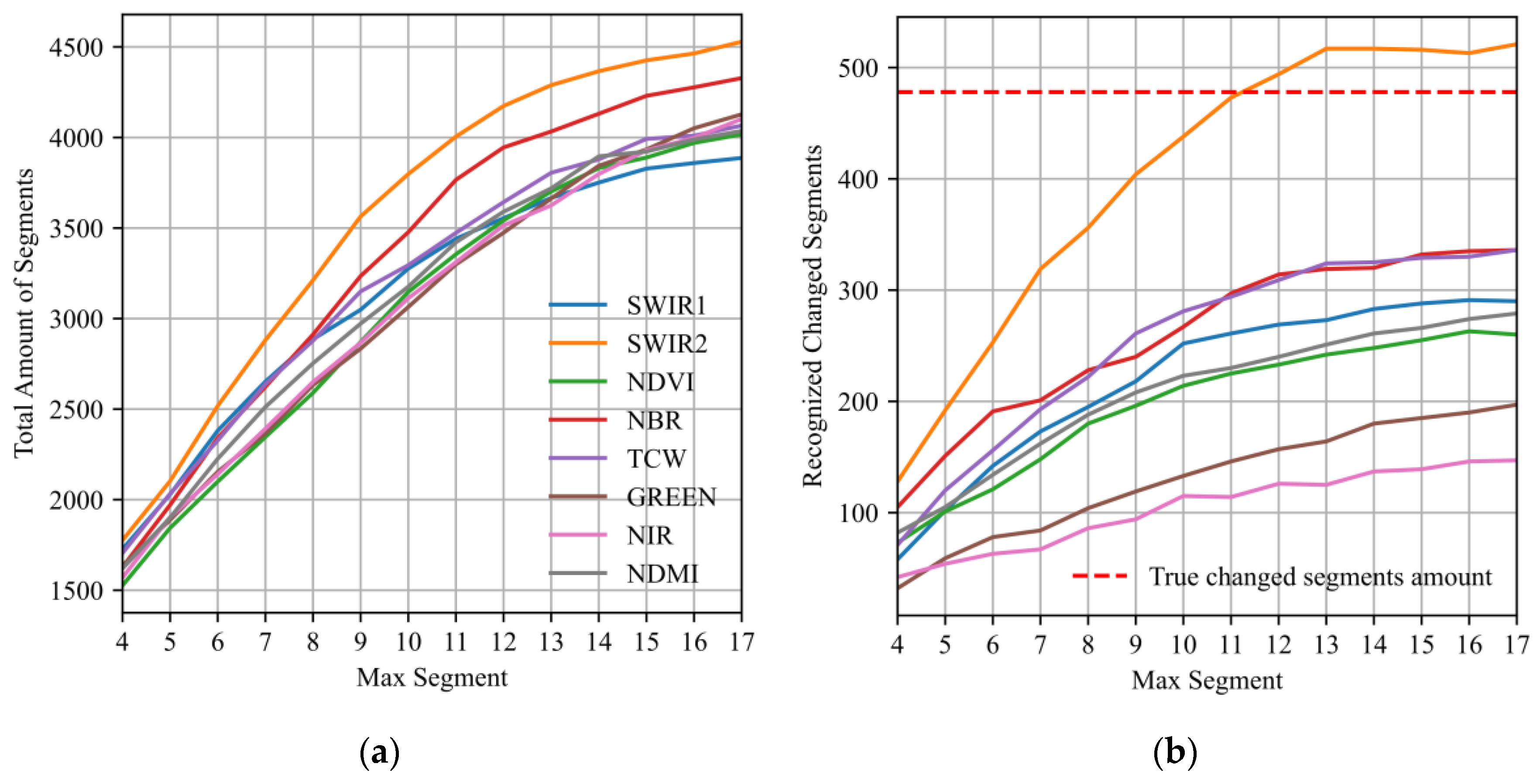
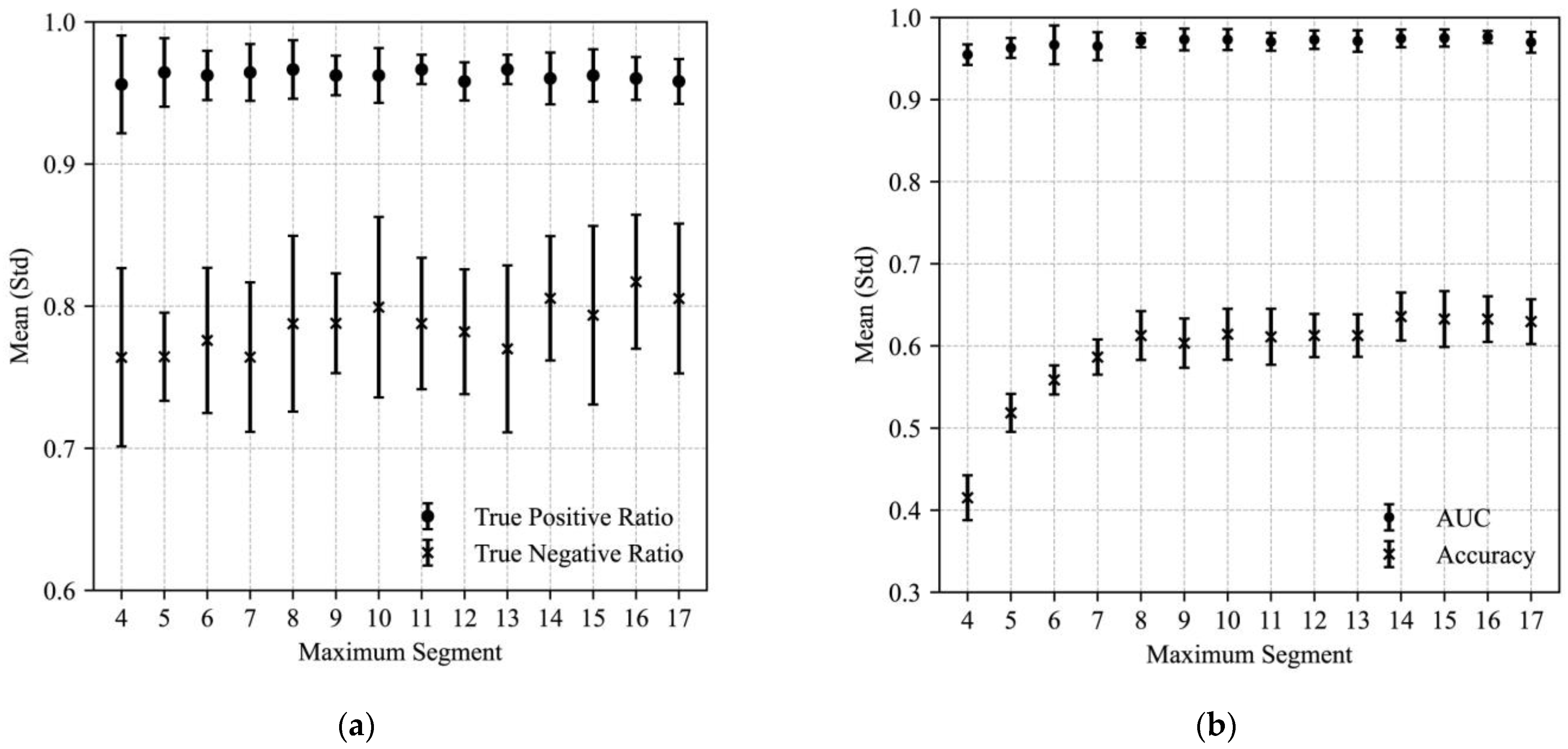
3.1. Filtering Performance of the Baseline Methods
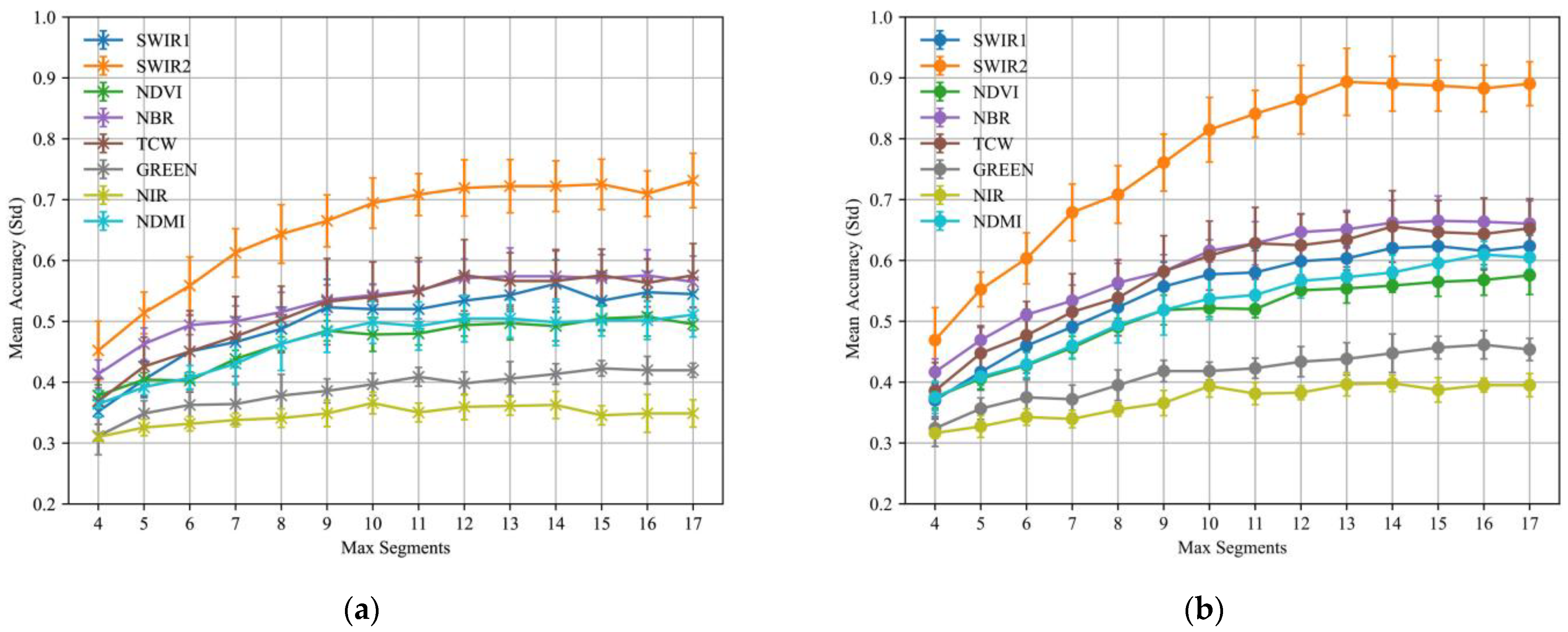
3.2. Filtering Performance of the Improved Methods
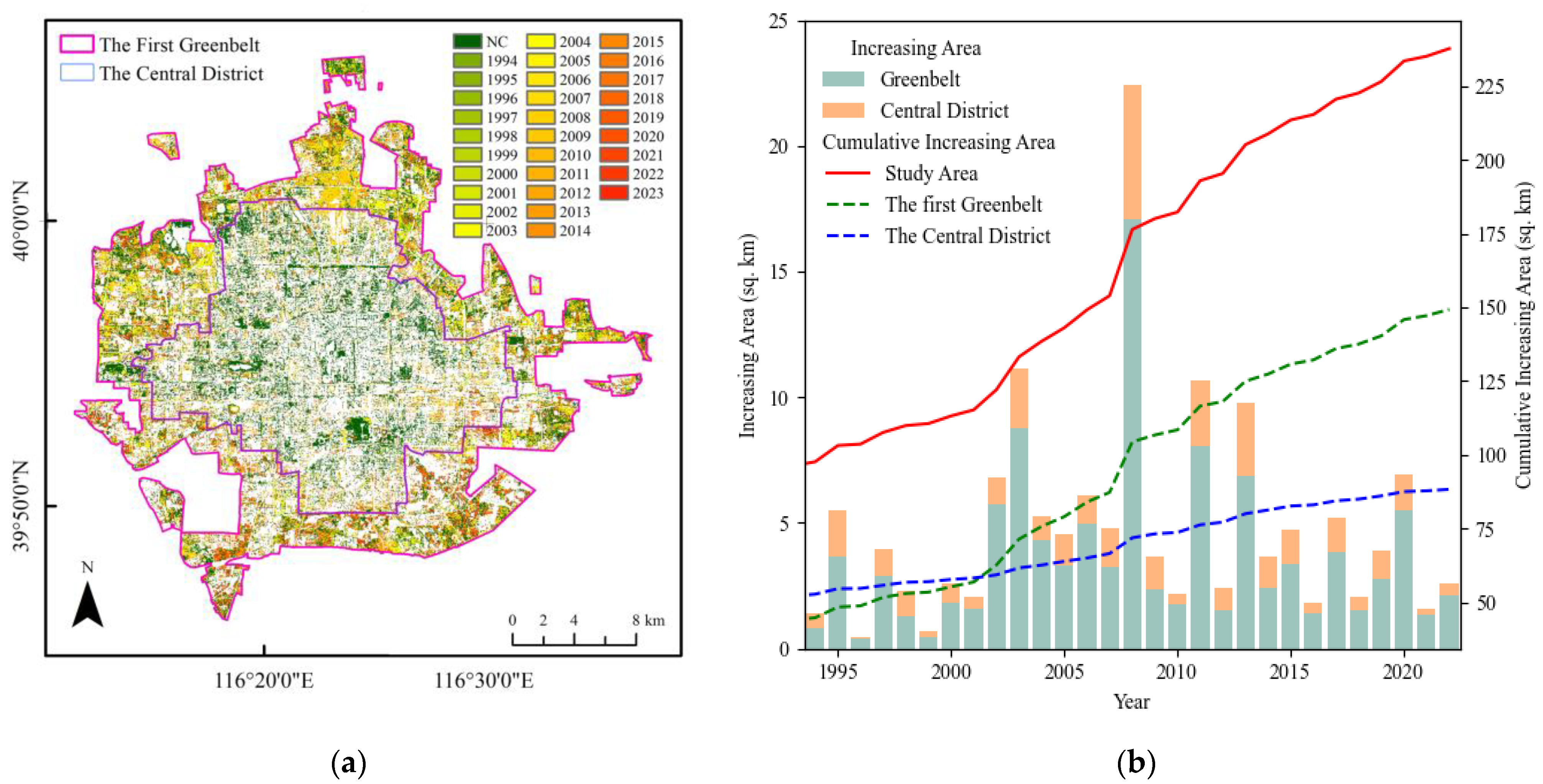
3.3. The Expansion Dynamic Mapping of Urban Forests in the Study Area
4. Discussion
4.1. Characteristics of the Improved Methods
4.2. Bands/Indices and Parameter Optimization for Urban Forest Detection
4.3. Annual Dynamics Benefit Urban Forest Management
4.4. Limitations
5. Conclusions
Author Contributions
Funding
Data Availability Statement
Conflicts of Interest
Appendix A

| Ranking | Name | Feature Importance | Selected Features |
|---|---|---|---|
| 1 | Rates | 0.1265 | ✓ |
| 2 | DSNR | 0.0647 | ✓ |
| 3 | Magnitude | 0.0564 | ✓ |
| 4 | SD_endvalue_post_rank | 0.056 | ✓ |
| 5 | Rates_rank | 0.0467 | ✓ |
| 6 | SD_endvalue_post | 0.0419 | ✓ |
| 7 | SD_rate_post | 0.0383 | ✓ |
| 8 | Start_value | 0.0373 | ✓ |
| 9 | Avr_mag_pre | 0.0314 | ✓ |
| 10 | SD_mags_post_rank | 0.031 | ✓ |
| 11 | Avr_endvalue_post_rank | 0.0306 | ✓ |
| 12 | SD_mags_post | 0.0291 | ✓ |
| 13 | DSNR_rank | 0.0284 | ✓ |
| 14 | Magnitude_rank | 0.0252 | ✓ |
| 15 | Avr_endvalue_post | 0.0209 | ✓ |
| 16 | SD_rate_post_rank | 0.0192 | ✓ |
| 17 | Avr_mag_pre_rank | 0.0186 | ✓ |
| 18 | Start_value_rank | 0.0156 | ✓ |
| 19 | Duration | 0.0154 | ✓ |
| 20 | DSNR_min | 0.0131 | ✓ |
| 21 | SD_mags_post_min | 0.0129 | ✓ |
| 22 | Mag_post | 0.0129 | ✓ |
| 23 | Rate_post | 0.0126 | ✓ |
| 24 | Rates_min | 0.0124 | ✓ |
| 25 | Magnitude_min | 0.0103 | ✓ |
| 26 | Avr_rate_pre | 0.0099 | ✓ |
| 27 | SD_rate_post_min | 0.0097 | ✓ |
| 28 | Avr_rate_pre_rank | 0.0095 | |
| 29 | Avr_startvalue_pre | 0.0092 | ✓ |
| 30 | Mag_pre | 0.009 | ✓ |
| 31 | Start_value_max | 0.0085 | |
| 32 | SD_endvalue_post_min | 0.0084 | ✓ |
| 33 | Rate_pre | 0.0076 | ✓ |
| 34 | Avr_startvalue_pre_rank | 0.0072 | |
| 35 | SD_startvalue_pre | 0.0067 | |
| 36 | Avr_rate_post | 0.0063 | ✓ |
| 37 | Rate_post_rank | 0.0061 | |
| 38 | Avr_mag_post | 0.0061 | ✓ |
| 39 | End_value | 0.006 | ✓ |
| 40 | SD_rate_pre | 0.0057 | |
| 41 | SD_mags_pre | 0.0053 | |
| 42 | Mag_pre_rank | 0.0049 | |
| 43 | Mag_post_rank | 0.0049 | |
| 44 | Rate_pre_rank | 0.0045 | |
| 45 | Avr_rate_post_rank | 0.0044 | |
| 46 | Avr_mag_post_rank | 0.0044 | |
| 47 | SD_startvalue_pre_rank | 0.0043 | |
| 48 | SD_rate_pre_rank | 0.0034 | |
| 49 | SD_mags_pre_rank | 0.003 | |
| 50 | Avr_mag_pre_min | 0.003 | ✓ |
| 51 | Duration_rank | 0.003 | |
| 52 | End_value_rank | 0.0028 | |
| 53 | Avr_rate_post_min | 0.0026 | |
| 54 | Avr_mag_post_min | 0.0021 | |
| 55 | Avr_mag_pre_max | 0.002 | |
| 56 | Rate_post_min | 0.0019 | |
| 57 | Duration_max | 0.0017 | |
| 58 | Duration_min | 0.0017 | |
| 59 | Avr_endvalue_post_min | 0.0016 | ✓ |
| 60 | SD_startvalue_pre_min | 0.0015 | |
| 61 | End_value_max | 0.0014 | |
| 62 | Avr_rate_pre_max | 0.001 | |
| 63 | SD_rate_pre_min | 0.0008 | |
| 64 | Avr_rate_pre_min | 0.0008 | |
| 65 | SD_mags_pre_min | 0.0007 | |
| 66 | SD_mags_pre_max | 0.0006 | |
| 67 | SD_startvalue_pre_max | 0.0006 | |
| 68 | Mag_post_min | 0.0006 | |
| 69 | SD_endvalue_post_max | 0.0006 | |
| 70 | Mag_pre_max | 0.0005 | |
| 71 | End_value_min | 0.0005 | |
| 72 | Rate_pre_min | 0.0005 | |
| 73 | Avr_startvalue_pre_min | 0.0005 | |
| 74 | Rate_pre_max | 0.0005 | |
| 75 | DSNR_max | 0.0005 | |
| 76 | Avr_startvalue_pre_max | 0.0005 | |
| 77 | Avr_rate_post_max | 0.0004 | |
| 78 | SD_mags_post_max | 0.0004 | |
| 79 | Mag_post_max | 0.0003 | |
| 80 | Mag_pre_min | 0.0003 | |
| 81 | Avr_mag_post_max | 0.0003 | |
| 82 | Rate_post_max | 0.0003 | |
| 83 | SD_rate_post_max | 0.0003 | |
| 84 | SD_rate_pre_max | 0.0003 | |
| 85 | Rates_max | 0.0002 | |
| 86 | Start_value_min | 0.0002 | ✓ |
| 87 | Avr_endvalue_post_max | 0.0001 | |
| 88 | Magnitude_max | 0 |

| Real Value Projected Value | Evergreen Trees | Deciduous Trees | Grass | Water Bodies | Impervious Surfaces |
|---|---|---|---|---|---|
| Evergreen trees | 65 | 14 | 2 | 1 | 0 |
| Deciduous trees | 5 | 48 | 9 | 2 | 0 |
| Grassland | 7 | 3 | 54 | 1 | 0 |
| Water bodies | 2 | 1 | 0 | 80 | 1 |
| Impervious surfaces | 0 | 0 | 4 | 2 | 64 |
| Producer accuracy (PA) | 0.79 | 0.75 | 0.83 | 0.95 | 0.91 |
| User accuracy (UA) | 0.82 | 0.73 | 0.78 | 0.93 | 0.98 |
| Overall accuracy (OA) | 0.85 | ||||
| Kappa index | 0.81 | ||||
References
- Yao, N.; Konijnendijk van den Bosch, C.C.; Yang, J.; Devisscher, T.; Wirtz, Z.; Jia, L.; Duan, J.; Ma, L. Beijing’s 50 Million New Urban Trees: Strategic Governance for Large-Scale Urban Afforestation. Urban For. Urban Green. 2019, 44, 126392. [Google Scholar] [CrossRef]
- Sun, L.; Chen, J.; Li, Q.; Huang, D. Dramatic Uneven Urbanization of Large Cities throughout the World in Recent Decades. Nat. Commun. 2020, 11, 5366. [Google Scholar] [CrossRef] [PubMed]
- Cadaval, S.; Clarke, M.; Roman, L.A.; Conway, T.M.; Koeser, A.K.; Eisenman, T.S. Managing Urban Trees through Storms in Three United States Cities. Landsc. Urban Plan. 2024, 248, 105102. [Google Scholar] [CrossRef]
- Shen, G.; Wang, Z.; Liu, C.; Han, Y. Mapping Aboveground Biomass and Carbon in Shanghai’s Urban Forest Using Landsat ETM+ and Inventory Data. Urban For. Urban Green. 2020, 51, 126655. [Google Scholar] [CrossRef]
- Zhuang, Q.; Shao, Z.; Gong, J.; Li, D.; Huang, X.; Zhang, Y.; Xu, X.; Dang, C.; Chen, J.; Altan, O.; et al. Modeling Carbon Storage in Urban Vegetation: Progress, Challenges, and Opportunities. Int. J. Appl. Earth Obs. Geoinf. 2022, 114, 103058. [Google Scholar] [CrossRef]
- Lin, J.; Kroll, C.N.; Nowak, D.J.; Greenfield, E.J. A Review of Urban Forest Modeling: Implications for Management and Future Research. Urban For. Urban Green. 2019, 43, 126366. [Google Scholar] [CrossRef]
- Hilbert, D.R.; Roman, L.A.; Koeser, A.K.; Vogt, J.; Doorn, N.S. Urban Tree Mortality: A Literature Review. Arboric. Urban For. 2019, 45, 167–200. [Google Scholar] [CrossRef]
- Wang, J.; Zhou, W.; Qian, Y.; Li, W.; Han, L. Quantifying and Characterizing the Dynamics of Urban Greenspace at the Patch Level: A New Approach Using Object-Based Image Analysis. Remote Sens. Environ. 2018, 204, 94–108. [Google Scholar] [CrossRef]
- Chen, W.; Huang, H.; Dong, J.; Zhang, Y.; Tian, Y.; Yang, Z. Social Functional Mapping of Urban Green Space Using Remote Sensing and Social Sensing Data. ISPRS J. Photogramm. Remote Sens. 2018, 146, 436–452. [Google Scholar] [CrossRef]
- Yang, Z.; Fang, C.; Li, G.; Mu, X. Integrating Multiple Semantics Data to Assess the Dynamic Change of Urban Green Space in Beijing, China. Int. J. Appl. Earth Obs. Geoinf. 2021, 103, 102479. [Google Scholar] [CrossRef]
- Yang, J.; Jinxing, Z. The Failure and Success of Greenbelt Program in Beijing. Urban For. Urban Green. 2007, 6, 287–296. [Google Scholar] [CrossRef]
- Zhu, Z. Change Detection Using Landsat Time Series: A Review of Frequencies, Preprocessing, Algorithms, and Applications. ISPRS J. Photogramm. Remote Sens. 2017, 130, 370–384. [Google Scholar] [CrossRef]
- Zhu, Z.; Woodcock, C.E.; Olofsson, P. Continuous Monitoring of Forest Disturbance Using All Available Landsat Imagery. Remote Sens. Environ. 2012, 122, 75–91. [Google Scholar] [CrossRef]
- Verbesselt, J.; Zeileis, A.; Herold, M. Near Real-Time Disturbance Detection Using Satellite Image Time Series. Remote Sens. Environ. 2012, 123, 98–108. [Google Scholar] [CrossRef]
- Kennedy, R.E.; Yang, Z.; Cohen, W.B. Detecting Trends in Forest Disturbance and Recovery Using Yearly Landsat Time Series: 1. LandTrendr—Temporal Segmentation Algorithms. Remote Sens. Environ. 2010, 114, 2897–2910. [Google Scholar] [CrossRef]
- Cohen, W.B.; Yang, Z.; Healey, S.P.; Kennedy, R.E.; Gorelick, N. A LandTrendr Multispectral Ensemble for Forest Disturbance Detection. Remote Sens. Environ. 2018, 205, 131–140. [Google Scholar] [CrossRef]
- Shen, J.; Chen, G.; Hua, J.; Huang, S.; Ma, J. Contrasting Forest Loss and Gain Patterns in Subtropical China Detected Using an Integrated LandTrendr and Machine-Learning Method. Remote Sens. 2022, 14, 3238. [Google Scholar] [CrossRef]
- Kennedy, R.E.; Yang, Z.; Gorelick, N.; Braaten, J.; Cavalcante, L.; Cohen, W.B.; Healey, S. Implementation of the LandTrendr Algorithm on Google Earth Engine. Remote Sens. 2018, 10, 691. [Google Scholar] [CrossRef]
- Mugiraneza, T.; Nascetti, A.; Ban, Y. Continuous Monitoring of Urban Land Cover Change Trajectories with Landsat Time Series and LandTrendr-Google Earth Engine Cloud Computing. Remote Sens. 2020, 12, 2883. [Google Scholar] [CrossRef]
- Shimizu, K.; Murakami, W.; Furuichi, T.; Estoque, R.C. Mapping Land Use/Land Cover Changes and Forest Disturbances in Vietnam Using a Landsat Temporal Segmentation Algorithm. Remote Sens. 2023, 15, 851. [Google Scholar] [CrossRef]
- Ni, H.; Yu, L.; Gong, P.; Li, X.; Zhao, J. Urban Renewal Mapping: A Case Study in Beijing from 2000 to 2020. J. Remote Sens. 2023, 3, 0072. [Google Scholar] [CrossRef]
- Zhang, X.; Brandt, M.; Tong, X.; Tong, X.; Zhang, W.; Fensholt, R. Urban Core Greening Balances Browning in Urban Expansion Areas in China during Recent Decades. J. Remote Sens. 2024, 4, 0112. [Google Scholar] [CrossRef]
- Sun, L.; Fertner, C.; Jørgensen, G. Beijing’s First Green Belt—A 50-Year Long Chinese Planning Story. Land 2021, 10, 969. [Google Scholar] [CrossRef]
- State Council of the People’s Republic of China and Beijing Municipal Government. Beijing City Master Plan (2016–2035); State Council of the People’s Republic of China and Beijing Municipal Government: Beijing, China, 2017. [Google Scholar]
- Crawford, C.J.; Roy, D.P.; Arab, S.; Barnes, C.; Vermote, E.; Hulley, G.; Gerace, A.; Choate, M.; Engebretson, C.; Micijevic, E.; et al. The 50-Year Landsat Collection 2 Archive. Sci. Remote Sens. 2023, 8, 100103. [Google Scholar] [CrossRef]
- Flood, N. Seasonal Composite Landsat TM/ETM+ Images Using the Medoid (a Multi-Dimensional Median). Remote Sens. 2013, 5, 6481–6500. [Google Scholar] [CrossRef]
- Pasquarella, V.J.; Arévalo, P.; Bratley, K.H.; Bullock, E.L.; Gorelick, N.; Yang, Z.; Kennedy, R.E. Demystifying LandTrendr and CCDC Temporal Segmentation. Int. J. Appl. Earth Obs. Geoinf. 2022, 110, 102806. [Google Scholar] [CrossRef]
- Li, X.; Zhou, Y.; Zhu, Z.; Liang, L.; Yu, B.; Cao, W. Mapping Annual Urban Dynamics (1985–2015) Using Time Series of Landsat Data. Remote Sens. Environ. 2018, 216, 674–683. [Google Scholar] [CrossRef]
- Crist, E.P. A TM Tasseled Cap Equivalent Transformation for Reflectance Factor Data. Remote Sens. Environ. 1985, 17, 301–306. [Google Scholar] [CrossRef]
- Key, C.H.; Benson, N.C. Landscape Assessment (LA). FIREMON Fire Eff. Monit. Inventory Syst. 2006, 164, LA-1–LA-55. [Google Scholar]
- Rouse, J.W.; Haas, R.H.; Schell, J.A.; Deering, D.W. Monitoring Vegetation Systems in the Great Plains with ERTS. NASA Spec. Publ. 1974, 351, 309. [Google Scholar]
- Wilson, E.H.; Sader, S.A. Detection of Forest Harvest Type Using Multiple Dates of Landsat TM Imagery. Remote Sens. Environ. 2002, 80, 385–396. [Google Scholar] [CrossRef]
- Breiman, L. Random Forests. Mach. Learn. 2001, 45, 5–32. [Google Scholar] [CrossRef]
- Belgiu, M.; Drăguţ, L. Random Forest in Remote Sensing: A Review of Applications and Future Directions. ISPRS J. Photogramm. Remote Sens. 2016, 114, 24–31. [Google Scholar] [CrossRef]
- Lobo, J.M.; Jiménez-Valverde, A.; Real, R. AUC: A Misleading Measure of the Performance of Predictive Distribution Models. Glob. Ecol. Biogeogr. 2008, 17, 145–151. [Google Scholar] [CrossRef]
- Pal, M. Random Forest Classifier for Remote Sensing Classification. Int. J. Remote Sens. 2005, 26, 217–222. [Google Scholar] [CrossRef]
- Ma, M.; Jin, Y. What If Beijing Had Enforced the 1st or 2nd Greenbelt?—Analyses from an Economic Perspective. Landsc. Urban Plan. 2019, 182, 79–91. [Google Scholar] [CrossRef]
- Li, F.; Zheng, W.; Wang, Y.; Liang, J.; Xie, S.; Guo, S.; Li, X.; Yu, C. Urban Green Space Fragmentation and Urbanization: A Spatiotemporal Perspective. Forests 2019, 10, 333. [Google Scholar] [CrossRef]
- Ren, Z.; Zheng, H.; He, X.; Zhang, D.; Shen, G.; Zhai, C. Changes in Spatio-Temporal Patterns of Urban Forest and Its above-Ground Carbon Storage: Implication for Urban CO2 Emissions Mitigation under China’s Rapid Urban Expansion and Greening. Environ. Int. 2019, 129, 438–450. [Google Scholar] [CrossRef]
- Nicese, F.P.; Colangelo, G.; Comolli, R.; Azzini, L.; Lucchetti, S.; Marziliano, P.A.; Sanesi, G. Estimating CO2 Balance through the Life Cycle Assessment Prism: A—Study in an Urban Park. Urban For. Urban Green. 2021, 57, 126869. [Google Scholar] [CrossRef]
- Biocca, M.; Gallo, P.; Sperandio, G. Potential Availability of Wood Biomass from Urban Trees: Implications for the Sustainable Management of Maintenance Yards. Sustainability 2022, 14, 11226. [Google Scholar] [CrossRef]


| Index | Formulation | Reference |
|---|---|---|
| TCW | 0.0315 × Blue + 0.2021 × Green + 0.3102 × Red + 0.1594 ∗ NIR + − 0.6806 × SWIR1 − 0.6109 × SWIR2 | [29] |
| NBR | (NIR − Red)/(NIR + Red) | [30] |
| NDVI | (NIR − SWIR2)/(NIR + SWIR2) | [31] |
| NDMI | (NIR − SWIR1)/(NIR + SWIR1) | [32] |
| Category | Name | Variable Type |
|---|---|---|
| Basic Feature | Start_value, End_value, Duration, Rates, Magnitude, DSNR | Numeric |
| Trend Variation | SD_rate_post, SD_startvalue_pre, SD_endvalue_post, SD_mags_post, Rate_pre, Rate_post, Mag_pre, Mag_post, Avr_rate_pre, Avr_rate_post, Avr_mag_pre, Avr_mag_post, Avr_startvalue_pre, Avr_endvalue_post | Numeric |
| Extremum | Startvalue_min, Rates_min, Magnitude_min, SD_rate_post_min, SD_endvalue_post_min, SD_mags_post_min, Avr_mag_pre_min, Avr_endvalue_post_min, DSNR_min | Boolean |
| Ranking | Startvalue_rank, Rates_rank, Magnitude_rank, SD_rate_post_rank, SD_endvalue_post_rank, SD_mags_post_rank, Avr_mag_pre_rank, Avr_endvalue_post_rank, DSNR_rank | Categorical |
| Fold | TP | TN | FP | FN | Accuracy |
|---|---|---|---|---|---|
| 1 | 75 | 39 | 19 | 29 | 70.37% |
| 2 | 81 | 40 | 20 | 21 | 74.69% |
| 3 | 81 | 42 | 18 | 21 | 75.93% |
| 4 | 65 | 39 | 23 | 35 | 64.20% |
| Fold | TP | TN | FP | FN | Accuracy |
|---|---|---|---|---|---|
| 1 | 103 | 37 | 16 | 6 | 86.42% |
| 2 | 114 | 39 | 6 | 3 | 94.44% |
| 3 | 111 | 41 | 6 | 4 | 93.83% |
| 4 | 95 | 39 | 18 | 10 | 82.72% |
| Region | Area | Original | Expanded | Current | |||
|---|---|---|---|---|---|---|---|
| Area | Rate | Area | Rate | Area | Rate | ||
| The Central District | 312.53 | 52.19 | 16.70% | 36.15 | 11.57% | 88.34 | 28.27% |
| The 1st Greenbelt | 322.45 | 44.07 | 13.67% | 105.20 | 32.62% | 149.27 | 46.29% |
| Total | 634.98 | 96.26 | 15.16% | 141.35 | 22.26% | 237.61 | 37.42% |
Disclaimer/Publisher’s Note: The statements, opinions and data contained in all publications are solely those of the individual author(s) and contributor(s) and not of MDPI and/or the editor(s). MDPI and/or the editor(s) disclaim responsibility for any injury to people or property resulting from any ideas, methods, instructions or products referred to in the content. |
© 2024 by the authors. Licensee MDPI, Basel, Switzerland. This article is an open access article distributed under the terms and conditions of the Creative Commons Attribution (CC BY) license (https://creativecommons.org/licenses/by/4.0/).
Share and Cite
Liu, Z.; Zhang, Y.; Zheng, X. Improving Urban Forest Expansion Detection with LandTrendr and Machine Learning. Forests 2024, 15, 1452. https://doi.org/10.3390/f15081452
Liu Z, Zhang Y, Zheng X. Improving Urban Forest Expansion Detection with LandTrendr and Machine Learning. Forests. 2024; 15(8):1452. https://doi.org/10.3390/f15081452
Chicago/Turabian StyleLiu, Zhe, Yaru Zhang, and Xi Zheng. 2024. "Improving Urban Forest Expansion Detection with LandTrendr and Machine Learning" Forests 15, no. 8: 1452. https://doi.org/10.3390/f15081452
APA StyleLiu, Z., Zhang, Y., & Zheng, X. (2024). Improving Urban Forest Expansion Detection with LandTrendr and Machine Learning. Forests, 15(8), 1452. https://doi.org/10.3390/f15081452