Abstract
Vegetation canopy water content (CWC) crucially affects stomatal conductance and photosynthesis and, consequently, is a key state variable in advanced ecosystem models. Remote sensing has been shown to be an effective tool for retrieving CWCs. However, the retrieval of the CWC from satellite remote sensing data is affected by the vegetation canopy structure and soil background. This study proposes a methodology that combines a modified spectral down-scaling model with a high-universality leaf water content inversion model to retrieve the CWC through constraining the impacts of canopy structure and soil background on CWC retrieval. First, canopy spectra acquired by satellite sensors were down-scaled to leaf reflectance spectra according to the probabilities of viewing the sunlit foliage (PT) and background (PG) and the estimated spectral multiple scattering factor (M). Then, leaf water content, or equivalent water thickness (EWT), was obtained from the down-scaled leaf reflectance spectra via a leaf-scale EWT inversion model calibrated with PROSPECT simulation data. Finally, the CWC was calculated as the product of the estimated leaf EWT and canopy leaf area index. Validation of this coupled model was performed using satellite-ground synchronous observation data across various vegetation types within the study area, affirming the model’s broad applicability. Results indicate that the modified spectral down-scaling model accurately retrieves leaf reflectance spectra, aligning closely with site-level measured spectra. Compared to the direct inversion approach, which performs poorly with Hyperion satellite images, the down-scale strategy notably excels. Specifically, the Similarity Water Index (SWI)-based canopy EWT coupled model achieved the most precise estimation, with a normalized Root Mean Square Error (nRMSE) of 15.28% and an adjusted R2 of 0.77, surpassing the performance of the best index Shortwave Angle Normalized Index (SANI)-based model (nRMSE = 15.61%, adjusted R2 = 0.52). Given its calibration using simulated data, this coupled model proved to be a potent method for extracting canopy EWT from satellite imagery, suggesting its applicability to retrieve other vegetative biochemical components from satellite data.
1. Introduction
Vegetation canopy water content (CWC) significantly influences plant growth, the cycles of water and carbon, along with ecological dynamics, and is an important parameter of ecosystem models [1,2]. Traditional methods for measuring the CWC are often post-event, destructive, and, therefore, not suited for real-time, large-scale monitoring due to poor timeliness and extensive resource requirements [3,4]. Remote sensing technology addresses these limitations, offering a non-invasive, efficient means for real-time, large-scale dynamic monitoring and regional assessments [5,6].
Remote sensing techniques mark a significant advancement over traditional methods in retrieving CWC [7,8]. These methods can be broadly grouped into three main categories:
- (1)
- Vegetation Indices Approach: Combining reflectances from visible and near-infrared (NIR) or shortwave infrared (SWIR) bands to create indices, such as the Normalized Difference Vegetation Index (NDVI) [7,9]. However, the NDVI primarily reflects chlorophyll content and tends to saturate at high vegetation coverage, limiting its suitability for water content estimation [10,11]. Other indices orientated for monitoring water content have been developed, such as the Normalized Difference Water Index (NDWI), Shortwave Angle Normalized Index (SANI), and Shortwave Angle Slope Index (SASI) [6,8,10,12,13,14].
- (2)
- Radiative Transfer Models: These models simulate radiative transfer processes within the canopy to allow the analysis of mixed signals from vegetation and its background, and from the separated vegetation signal, leaf biochemical parameters can be retrieved [15]. Accurate remote sensing inversion of the CWC needs to separate the impacts of the canopy structure and soil background. Gao and Goetz [16,17] employed a spectral matching technique based on the Beer–Lambert law and the nonlinear least squares method to derive the CWC and other parameters by simulating canopy reflectance through iterative optimization. Similarly, Zarco-Tejada et al. [18] integrated the PROSPECT leaf model with the SAILH canopy radiation transmission model, optimizing calculations iteratively to constrain the effects of the canopy structure and soil background on CWC inversion. The PROSPECT model is a widely used approach to modeling the optical properties of leaves across the visible to NIR spectral regions based on their biophysical and biochemical characteristics. The SAILH (Scattering by Arbitrarily Inclined Leaves with Hotspot effect) model is an advanced radiative transfer model used to simulate the bidirectional reflectance of vegetative canopies. Its integration with the leaf optical properties model PROSPECT makes it an essential component in remote sensing for the accurate retrieval and interpretation of vegetation characteristics. These approaches have been successfully implemented for water content estimation in remote sensing imagery, demonstrating their applicability and effectiveness (e.g., [18,19]).
- (3)
- Signal Analysis Techniques: Utilizing signal analysis, such as wavelet decomposition, to extract information pertinent to water content from hyperspectral data [5,20]. This method requires high spectral resolution data and a solid understanding of the underlying principles for effective application.
Each method has its advantages and challenges. Vegetation indices are widely used due to their simplicity and theoretical basis, but they lack universality and accuracy across different times and spaces [21,22,23]. Radiative transfer models provide detailed spectral analysis but are hindered by their requirement for extensive input data and computational complexity. Signal analysis techniques offer precision but are limited by their high spectral data requirements and the need for specialized knowledge.
Overall, the radiative transfer models have the potential to be more universal than the other methods because they can consider the influences of the canopy structure and soil background. Key to the success of using radiative transfer models is the inversion of leaf reflectance spectra from canopy reflectance spectra using spectral down-scaling methods [18,24]. Zarco-Tejada et al. [18] examined the effects of the leaf area index (LAI) and observed geometric angles using the SAILH canopy radiation transfer model, inverting the leaf reflectance spectra from the canopy reflectance spectra through an optimization iteration technique. Zhang et al. [24] explored the impact of canopy structure parameters, sun-target-sensor geometry, and soil background reflectance using the 4-Scale Geometric Optical (GO) model, streamlining the calculation process by introducing a lookup table (LUT) for the inversion of leaf reflectance spectra from canopy reflectance spectra. While both approaches are grounded in the physical mechanisms of remote sensing, the latter enhances inversion calculation efficiency by utilizing LUTs to bypass the need for optimized iterative calculations. This advancement requires extensive model simulations to establish two LUTs, which capture canopy structure parameters and observation geometry as inputs for retrieving the three essential parameters, including the probability of viewing the sunlit leaves (PT), the probability of viewing the sunlit background (PG), and spectral multiple scattering factor (M), in the inversion process. However, the variability in canopy structure parameters and observation geometry over different pixels poses a significant challenge, making the task of individual pixel processing labor-intensive and less feasible for large-scale satellite remote sensing applications.
Despite advances in remote sensing techniques for estimating the CWC, there remain limitations in the accuracy, universality, and applicability of existing methods due to factors such as the canopy structure and soil background. These limitations highlight the need for innovative approaches that can integrate and improve upon existing methods.
This study refines spectral down-scaling inversion models to develop a down-scaling inversion strategy for estimating the CWC. By coupling the modified spectral down-scaling model with a leaf water content (LWC, or equivalent water thickness: EWT) inversion model, we constrain the influence of canopy structure and soil background on remote sensing inversion results of the LWC. First, the leaf reflectance spectra were inverted from the canopy spectra using the modified spectral down-scaling model. The LWC was then retrieved from the inverted leaf reflectance spectra using the leaf-scale inversion model. Finally, the CWC was calculated by multiplying the inverted LWC with the canopy LAI. Satellite-ground synchronous observation data for different vegetation types were used to validate the coupled model.
2. Materials and Methods
Satellite-ground synchronous in situ observation data offer a feasible means of validating the performance of the down-scaling inversion strategy for retrieving the CWC. Specific details for the dataset are provided in the following sections:
2.1. Study Area and Sampling
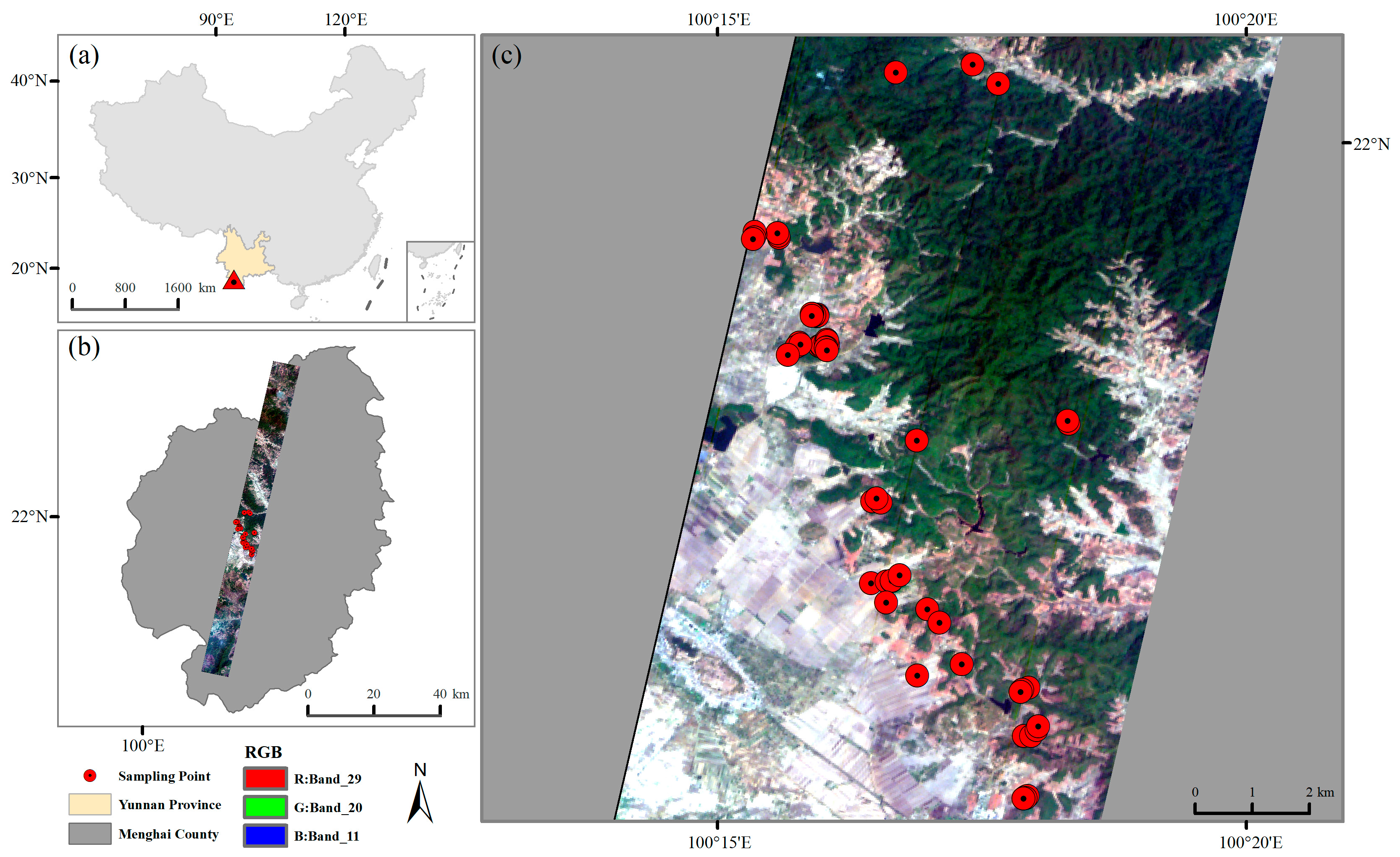
As shown in Figure 1, the center of the study area was located at Xishuangbanna (21.98° N, 100.29° E) in the Yunnan province, southwest China. Xishuangbanna is located on the northern edge of the tropics. It is a mountainous landform in the southwest that is divided into three parts: the central mountains, hills, and basins. The climate is a tropical, subtropical southwest monsoon climate. Temperatures average 18.1 °C, and precipitation averages 1224.7 mm. It is the most intact tropical ecosystem in China, with a rich biodiversity of plant species. The forest vegetation in the study area is mainly secondary broad-leaved forests.

Figure 1.
Study area and sampling locations: (a) the study area was located in Menghai county (21.98° N, 100.29° E), Xishuangbanna, Yunnan province in southwest China. (b) The RGB true color image of Hyperion remote sensing data and (c) sampling points for ground synchronous observation.
Data were collected from 33 sites across 11 different vegetation types: pine (3), bamboo (3), tea plantations (4), corn (4), potato (3), flax (6), saccharose (4), chestnut trees (5), and mountain ephedra (1). Sample sites were large enough (90 m × 90 m) to match a pure pixel on the Hyperion image and carefully selected to be easily accessible by road [25,26].
We selected specific Hyperion pixels corresponding to our in situ measurement sites to ensure that the spectral data from the satellite image accurately matched the geographical locations of the ground measurements. Each pixel in the Hyperion image was carefully chosen to align with our study sites, thereby maintaining the accuracy and relevance of the spectral data.
2.2. Ground Synchronous Observation Parameters
From 25 to 31 March 2005, each sample site was measured to obtain leaf optical spectra (reflectance and transmission), along with biophysical and biochemical parameters, canopy structural parameters (including the LAI, tree crown radius, clumping index, stem density, and tree height), and the geographic location (longitude and latitude) using the WGS84 (World Geodetic System 1984) geographic coordinate system.
2.2.1. Leaf Optical Properties, Biophysical and Biochemical Parameters
Three representative plants were randomly selected at each site for leaf sample collection from the top, middle, and lower positions in the crown. Leaf hemispherical reflectance and transmission spectra were measured using the standard method with a FieldSpec® FR spectroradiometer (as referred to in [25]).
Using leaf samples collected at each site, the LWC and leaf area of the vegetation were measured. The averages of these leaf samples served as ground truth data to assess the accuracy of the retrieval results. About 3~5 leaves were selected from each sample; the fresh weight was measured by an electronic balance with an accuracy of 0.01 g and recorded as M1 (g). The measured leaves were laid flat on A4 white paper marked with 1 cm × 1 cm tac-toe, pressed against a thin glass sheet, photographed, and recorded with the serial number of the photos, and the total leaf area S (cm2) was calculated to obtain the fresh leaf density M1/S (g/cm2). Afterwards, the leaves were put into the oven to dry and were first dried at 105 °C for 30 min and then baked at 65 °C for 24 h. The leaves were collected, dried, and cooled in a dryer and then weighed and recorded. The difference in weight between the two times was the water content of the leaves. The corresponding fresh leaf density M1/S was used to calculate the concentration of biochemical parameters in the unit leaf area. The equivalent water thickness (EWT) was calculated using Equation (1) as follows:
The leaf chlorophyll content was measured using the standard method (referred to [27]) to determine the amount of chlorophyll in a leaf.
2.2.2. Canopy Structural Parameters and Soil Background Reflectance
Figure A1 in Appendix A shows that these 33 sites have two soil background types (red and gray soils) and different crown closures. Each forest site was marked with 5 to 10 medium-sized trees for measuring the average DBH (diameter at breast height) and tree height, and a count of individual trees was used to determine the stem density. The radius of the tree crown was measured by taking the average of two perpendicular crown diameters. The measurements were made using a measuring tape from the edge of the crown to the trunk in four cardinal directions. The clumping index (CI) was estimated by visual inspection and through the analysis of hemispherical photographs taken from beneath the canopy. The method to calculate canopy gap fractions from digital hemispherical photos (DHPs) can be referred to by J. Pisek et al. [28]. Then, we calculated the clumping index using the following Equation (2):
where Fm(0) is the measured total canopy gap fraction, and Fmr(0) is the total canopy gap fraction without the large gaps that cause no randomness of the canopy. Stem density was determined by counting the number of trees within a defined area (0.1 hectare) at each site. This value was then scaled to a per-hectare basis for standardization. Tree height was measured using a clinometer and a measuring tape. The observer stood a known distance from the tree and measured the angle of the ground to the top of the tree. Using trigonometry, the height of the tree was then calculated. The LAI at each site was measured with a Plant Canopy Analyzer (LAI-2000, Li-COR, Inc., Lincoln, NE, USA). Using Global Navigation Satellite System (GNSS) geographic coordinates (longitude and latitude) of the selected sites, 33 Hyperion pixels were selected, with each Hyperion pixel corresponding to one in situ site (Figure 1).
2.3. Hyper-Spectral Remote Sensing Imagery
At noon on 28 March 2005, a Hyperion remote sensing image was acquired. The image consisted of 242 channels with a 10 nm spectral resolution, covering visible, NIR, and SWIR wavelengths from 400 nm to 2500 nm (Table A1 in Appendix A) at a spatial resolution of 30 m. Image stripes and the Smile effect were repaired after bad pixels and invalid channels (Table A1 in Appendix A) were removed.
Atmospheric correction was performed for reflectance calculations. Image geometric correction was georeferenced based on a georeferenced Landsat Thematic Mapper (TM) image acquired on 16 February 2005. All root mean square errors (RMSEs) of the ground control points (GCPs) were within 0.35 pixels [25].
The 2005 Hyperion dataset was selected primarily due to the availability of comprehensive, synchronized ground-truth measurements, which were essential for validating the accuracy of our model results in the study area. In future work, we intend to apply our methodology to more recent satellite data to assess its performance and potential accuracy improvements. Furthermore, we will explore high-resolution datasets from newer satellite missions to further validate and refine our model.
2.4. Methodology
The aim of this study is to construct a down-scaling inversion strategy for retrieving the CWC, which integrates the modified spectral down-scaling model and the LWC inversion model. This integration is intended to alleviate the influence of canopy structure and soil background, with the ultimate goal of accurately estimating the CWC. The primary objective of down-scaling is to convert canopy-level reflectance spectra to leaf-level reflectance spectra, enabling more accurate estimation of the LWC and subsequently the CWC. The process involves several key steps, as detailed below: (1) Spectral Down-scaling: The canopy spectra are decomposed into leaf reflectance spectra by applying the down-scaling model, which accounts for the structural and optical properties of the canopy. Using our modified spectral down-scaling model, we convert the canopy reflectance spectra (measured at the 30 m × 30 m spatial resolution) to leaf reflectance spectra. (2) LWC Estimation: The EWT of the leaves was retrieved from the down-scaled leaf reflectance spectra using a leaf-scale EWT inversion model, which has been calibrated with PROSPECT simulated data. This step ensures that the water content at the leaf level is accurately estimated. (3) Calculation of the CWC: The estimated leaf EWT values are then combined with the LAI estimates at each site to calculate the overall CWC. This integration step translates the leaf-level EWT back to the canopy level, ensuring coherence with the initial spatial resolution of the satellite data. This dual-level approach (canopy to leaf and back to canopy) enhances the reliability and applicability of the retrieved water content data.
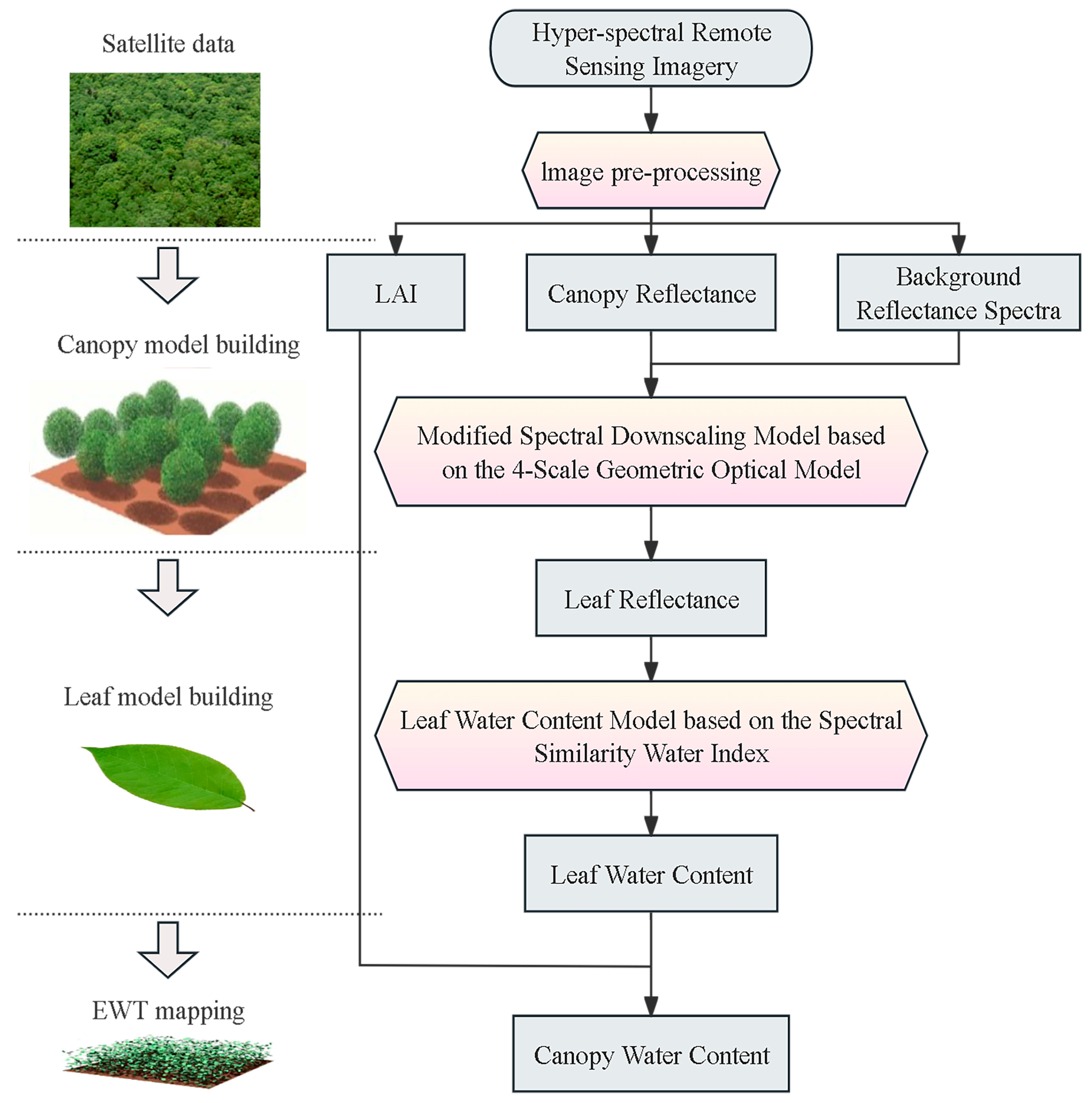
2.4.1. Coupled Down-Scaling Inversion Strategy
The workflow of the coupled down-scaling inversion strategy is illustrated in Figure 2. The specific steps involved in the process are as follows: (1) To preprocess the remote sensing image, including atmospheric correction, geometric correction, pixel classification, and masking of non-vegetation pixels, using Environment for Visualizing Images (ENVI) software (Version 5.3); (2) To retrieve LAI using an algorithm developed by Wu et al. [26]. This algorithm based on empirical relationships was calibrated using observations and the Modified Simple Ratio (MSR705) derived from the same Hyperion image [26]; (3) To determine soil reflectance. Since the study area primarily consists of gray soil and red soil, with gray soil being the predominant type, the reflectance of gray soil, as recorded in the soil spectral database, was utilized to represent the background reflectance of the study area; (4) To develop a modified spectral down-scaling model on the basis of the 4-Scale GO model [29] to estimate leaf reflectance using hyperspectral images from the satellite at the canopy level; (5) To retrieve the leaf-level mean water content through the application of the leaf-level Similarity Water Index (SWI)-based inversion model, utilizing the estimated leaf-level reflectance; (6) To calculate the canopy-level water content by multiplying the retrieved leaf water content with canopy LAI, as shown in Equation (3):
where is the mean LWC at the pixel scale (g/cm2), EWTcanopy is the CWC at the pixel scale (g/m2), and 104 is the unit conversion factor.

Figure 2.
Workflow of the coupled down-scaling inversion strategy retrieving leaf-level and canopy-level water content from satellite data considering canopy structure and background effects.
The estimated values from the coupled model were compared with the satellite-ground synchronous measurements obtained from site sampling. The comparison of estimated and actual leaf and canopy EWT was conducted using the nRMSE and the adjusted R2 ().
The nRMSE is calculated by the following Equation (4):
where EWTmax and EWTmin are the maximum and minimum EWT, respectively.
2.4.2. Four-Scale Geometric Optical (GO) Model
Chen and Leblanc’s [29] 4-Scale GO model assumed that canopy reflectance is a linear combination of four components/fractions: sunlit leaves, sunlit background, shaded leaves, and shaded background [29,30], as shown in Equation (5):
where is the canopy reflectance observed from satellites, and PT represent the reflectance of and the probability of viewing sunlit leaves, and ZT represent the reflectance of and the probability of viewing shaded leaves, and PG represent the reflectance of and the probability of viewing sunlit backgrounds, and ZG represent the reflectance of and the probability of viewing shaded backgrounds, respectively.
Therefore, the forward modeling process from the leaf spectrum to the canopy spectrum is divided into two steps. First, a simulated observation scene is established based on the input vegetation canopy structure parameters and observation geometric parameters, etc., and the probabilities of viewing these four components (PT, ZT, PG, and ZG) in the simulated scene are calculated. The structural effects were determined by the spatial distribution of tree groups, the geometry of tree crowns, tree branching, and scattering elements. Structural and angular variations in multiple scattering processes are simulated using a multiple scattering scheme that is based on the viewing factors of the four canopy components [31]. The canopy structural parameters were provided by field measurements at our study sites. The observation geometric parameters were determined from the Hyperion image.
Then, canopy reflectance spectra were simulated based on the input optical properties of leaf and forest backgrounds and the four canopy components of the observation scene [29,30]. The optical properties of leaf and forest backgrounds have been provided by field and laboratory measurements at our study sites. Table A2 in Appendix A lists the structural and other parameters incorporated in the 4-Scale GO model for the study sites. The corresponding canopy reflectance and probabilities of viewing sunlit and shaded fractions were estimated for each observation scene in the output.
2.4.3. Modified Spectral Down-Scaling Model
A modified spectral down-scaling model was proposed to invert the leaf reflectance spectrum using the canopy reflectance spectrum based on the 4-Scale GO model. In order to invert the leaf reflectance spectrum from the canopy reflectance spectrum, Zhang et al. [24] introduced a multiple scattering factor M and proposed a spectral down-scaling model based on the 4-Scale GO model, as expressed in Equation (6):
where is the individual leaf reflectivity, which is approximately equal to the reflectivity of sunlit foliage, while the former contains multiple scattering; , , PT, and PG have the same variable interpretation as in Equation (5). Multiple scattering factor M includes contributions from two shaded components and multiple scattering components.
Among the five input parameters of the spectral down-scaling model, canopy reflectance spectra are derived from satellite remote sensing images. Assuming that the background reflectance is known, the conversion of canopy reflectance spectra to single-leaf reflectance can be realized only by further calculating PT, PG, and M.
Theoretically, M can be calculated from the following Equation (7) [24]:
In practical application, M cannot be determined by the above equation because is unknown. In order to solve this problem, Zhang et al. [24] developed lookup tables (LUTs) based on the simulation results of the 4-Scale GO model to retrieve PT, PG, and M.
Given that canopy reflectance and forest background reflectivity can be measured remotely, it is necessary to estimate the PT, PG, and M parameters to invert the leaf reflectivity . The 4-Scale GO model was used to develop two LUTs to account for different canopy structures and viewing angles. In order to simplify the process, two LUTs were designed based on observation geometric parameters (VZA, SZA, and PHI) as well as LAI to estimate the PT and PG components and M factor, respectively. However, we found that there is no one-to-one correspondence between the variables in the lookup tables (see Section 3.1 and Figure 3), which would lead to an ill-conditioned retrieval problem.
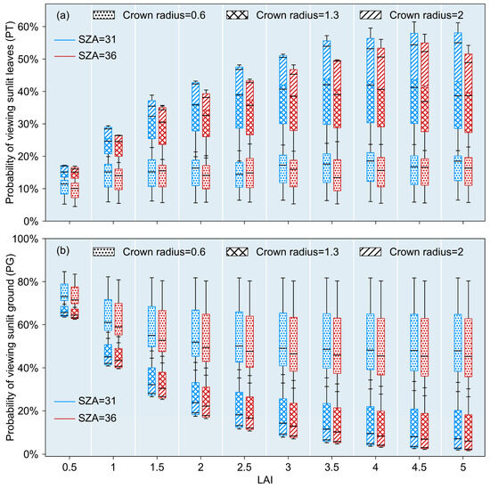
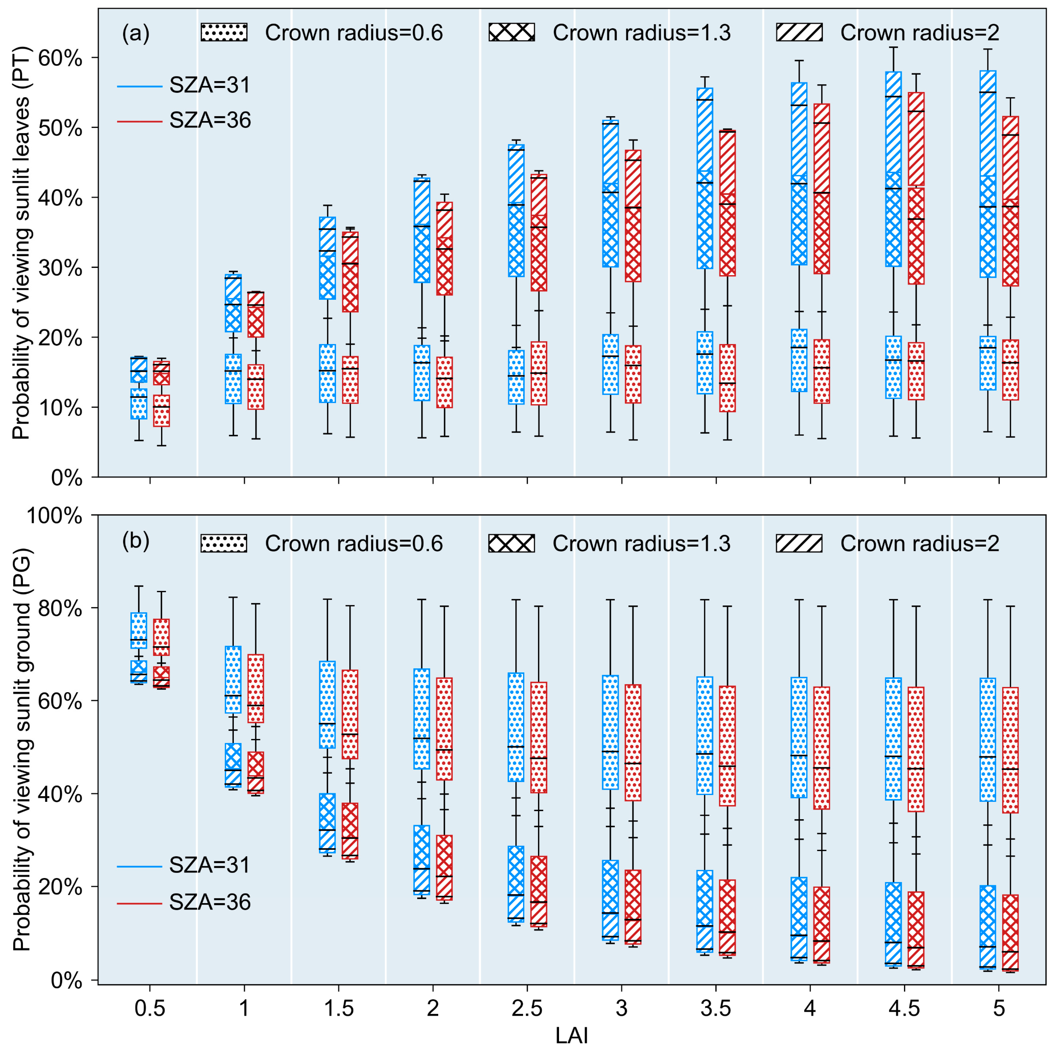
Figure 3.
Sensitivity of the simulated probability of viewing sunlit foliage (PT) (a) and sunlit background (PG) (b) to the solar zenith Angle (SZA), LAI and radius of tree crowns. Here, the tree density was set at 4000 trees per hectare and VZA = 0°.
To address this ill-conditioned retrieval issue inherent in the original LUT method, we have modified the LUT approach to make it more efficient. An estimation model based on the normalized spectral angle index (NSAI), which shows significant potential for estimating PT and PG from canopy spectra observed by satellites at the pixel level, replaced the traditional LUTs for PT and PG, enabling direct acquisition of high-precision PT and PG values from satellite canopy reflectance (see reference [25] and Section 3.2). As shown in Equation (7), the M value is computable utilizing PT, PG, canopy reflectance, single-leaf reflectance, and background reflectance. Analysis revealed that with PT, PG, and background reflectance held constant, the conversion relationship between canopy and single-leaf reflectance is primarily related to LAI. Therefore, when PT and PG are estimated, the M lookup table of the original down-scaling model can be adapted to utilize PT, PG, and LAI as search parameters, creating a new lookup table for M. In the initial phase of calibration for the NSAI-based PT and PG estimation model and to compute M values across various retrieval combinations, we employed the 4-Scale GO model. This model simulated the Hyperion canopy reflectance of the study area, with the simulation’s precision validated (as detailed in Table A3 in Appendix A). Based on the Hyperion simulation dataset, we calibrated and validated the NSAI-based PT and PG estimation models and constructed a new lookup table for M using PT, PG, and LAI as the retrieval items. The modified spectral down-scaling model not only solves the problems that existed before, but makes it simpler.
2.4.4. PT and PG Prediction Model
PT and PG are pivotal variables in the modified spectral down-scaling model. Fang et al. [25] introduced an effective method for estimating PT using the NSAI, which shows significant potential for estimating PT and PG. The NSAI was calculated based on a pixel-level canopy spectrum observed by satellites at the Red (645 nm), NIR (858 nm), and SWIR (1240 nm) wavelengths to estimate PT.
The efficacy of the NSAI-based PT model was corroborated using Hyperion data, revealing an nRMSE and an adjusted R2 for an estimated PT of 14.9% and 0.744, respectively [25]. Notably, the empirical NSAI-based PT model demonstrated strong transferability from simulated to in situ satellite data, underscoring its utility.
Theoretical analysis indicates that the NSAI is predominantly influenced by PT and PG. The relationship was further validated using the simulated data, and a strong correlation between these variables was observed (see Figure A2 in Appendix A). Building on this, the current study adopts the PT inversion model construction method described by Fang et al. [25] to also develop a PG inversion model based on the NSAI, aiming to enhance the precision of the results. The derived PT and PG values, in conjunction with the LAI, facilitate the determination of the spectral multiple scattering factor M using a lookup table. These values are then applied in conjunction with M as inputs into Equation (6) to translate canopy reflectance into single-leaf reflectance, optimizing the inversion process.
2.4.5. Leaf-Level Water Content Prediction Model
Fang et al. [32] introduced the spectral similarity water indices (SWIs) as a means to effectively estimate the LWC (EWT) by utilizing the Spectral Angle Cosine (SAC) of leaf reflectance spectra and the specific water absorption spectrum. In this study, the spectral intervals (970–1150 nm) have been chosen based on the spectral characteristics of Hyperion to calculate the SWI index using the following Equation (8):
where r and w are the vectors representing the reflectance spectra of the leaves and the specific water absorption spectrum, which are assumed to comprise reflectance components from the Hyperion bands within the spectral domain (970–1150 nm), with the number of bands denoted as L.
EWT can be predicted using the following Equation (9):
where a and b are the coefficients obtained by calibration.
In order to assess the retrieval performance of SWI-based EWT models on Hyperion remote sensing data, the measured reflectance of all samples was resampled to acquire Hyperion-equivalent spectra.
Moreover, the transferability of the SWIs-based EWT models from simulation to in situ data has also been tested using Hyperion-equivalent spectra simulated by the PROSPECT to calibrate the models and the measured data to test the models. For the comparison, the SWI indices and six commonly used spectral indices specifically designed to estimate vegetation water content were calculated using the Hyperion-equivalent spectra. These indices include the Maximum Difference Water Index (MDWI), NDWI, Normalized Difference Infrared Index (NDII), Moisture Stress Index (MSI), Shortwave Angle Slope Index (SASI), and SANI. The correlations between these indices and EWT were then analyzed.
The calibrated regression models were further applied to the Hyperion-equivalent spectra of all measured samples, and the measured LWC was used to verify the performance of the SWIs-based EWT models and the indices-based EWT models. The resultant and nRMSE values between the estimated and reference EWT were calculated.
3. Results
3.1. Influence of Viewing Geometry and Canopy Structural Parameters
The modified spectral down-scaling model pivots on two critical variables: the PT and PG components. These variables change with viewing geometry and the structural parameters of vegetation canopies. To evaluate the sensitivity of PT and PG to these factors, we employed the 4-Scale GO model for simulation scenarios. For the simulations, the observation zenith angle (VZA) was fixed at 0°, and the tree density was standardized at 4000 trees per hectare. We identified the solar zenith angle (SZA), the LAI, and the crown radius as sensitive variables. The LAI ranged from 0.5 to 5 in increments of 0.5. We examined two distinct SZAs—31 and 36 degrees, the minimum and maximum SZA for the Hyperion image—denoted by blue and red, respectively. The crown radius was categorized into three distinct values: 0.6, 1.3, and 2.
Figure 3 illustrates the influence of the canopy structure and solar zenith angle on PT and PG. With the increase in the LAI, PT increases, and PG decreases. Both trends of PT and PG change with the LAI, gradually leveling off as the LAI increases, indicating a threshold effect. These trends are consistent across different crown radii and solar zenith angles. However, with a larger crown radius (crown radius = 2), the trends of PT and PG with the increasing LAI become more pronounced, and the threshold effect occurs later. Moreover, at the smaller solar zenith angle (SZA = 31°), both PT and PG values are higher. Under the condition of a smaller crown radius, the distribution of PT is more concentrated. In contrast, with a larger crown radius, the distribution of PG is more concentrated. In summary, the size of the crown radius has a significant impact on PT and PG, and there is a threshold effect in the impact of the LAI on PT and PG; the influence of the solar zenith angle on PT and PG is also non-negligible. The relationships of these three main influencing factors with PT and PG are nonlinear, and they interact with each other. As such, the original lookup table method developed by Zhang et al. [24], which retrieves PT and PG values based on observation angles, the LAI, and crown radius, is fraught with considerable uncertainty when crown radius data are lacking because there is no one-to-one correspondence between the variables in the lookup tables, potentially leading to an ill-conditioned retrieval problem that results in a loss of the value of the variable in the lookup table.
3.2. PT and PG Estimation and Lookup Tables (LUTs) of M
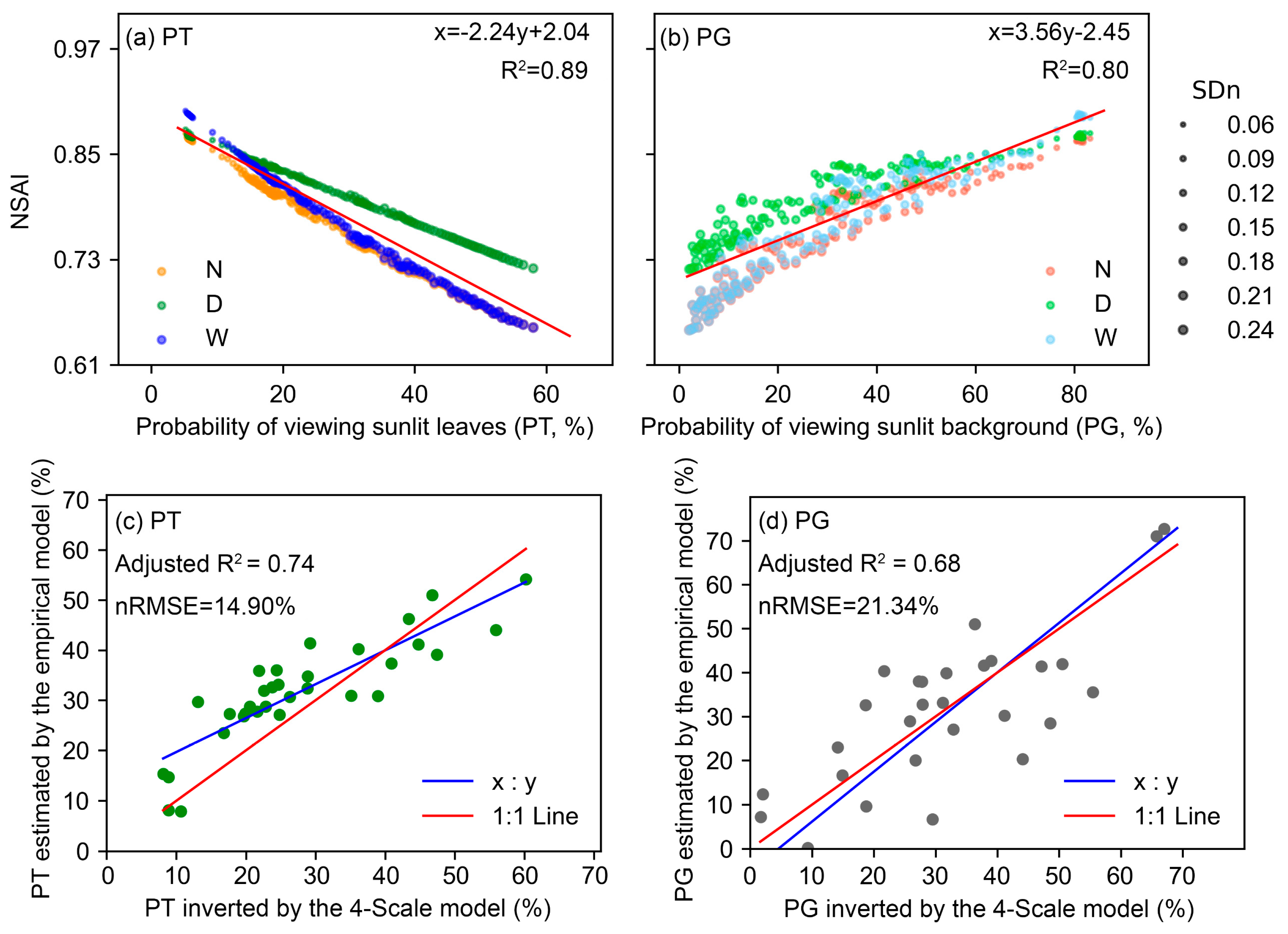
Leveraging the Hyperion simulation dataset, we have both calibrated and verified NSAI-based PT and PG estimation models (Figure 4), leading to the development of a novel M lookup table (wavelength dependent) that incorporates PT, PG, and the LAI as key retrieval elements (Table A4 in Appendix A).
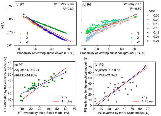
Figure 4.
Correlations of NSAI with PT (a) and PG (b) for the Hyperion synthetic data under conditions of normal soil (N, orange dots), dry soil (D, green dots), and wet soil (W, blue dots). A total of 13,950,144 Hyperion samples and 10,764 Hyperion scenes are available for analysis. On 33 Hyperion pixels, we compare PT (c) and PG (d) estimates using NSAI-based models to the reference values inverted with the 4-Scale GO model. The red straight lines are the 1:1 line. Correlations of NSAI with PT (a) and comparisons of PT estimated using NSAI with the reference values (c) are adapted from Fang et al. [25].
Figure 4 presents a comprehensive analysis of the relationship between the NSAI, PT, and PG alongside their respective model estimates. Figure 4a,b displays the relationship between PT and PG with the NSAI based on Hyperion synthetic data. To check for disturbance of the soil background variety, bubble scatter points are colored to represent the three soil background types (normal, dry, and wet). Normalized standard deviation (SDn = SD/Mean) of indices collected in the same scene is used to determine the size of bubble scatter plots. Despite having the same PT and PG, the variability in leaf spectra results in different index values, which is why we have different values for the same scene. The NSAI was linearly correlated to PT (Figure 4a) and PG (Figure 4b) with low SDn values. Soil background types had some effects on the linear relationship, but not very significant. Figure 4a,b provide the coefficients of calibrated regression models utilizing all soil backgrounds.
The calibrated regression models of all soil types were validated at the satellite level. The resultant and nRMSE between the estimated PT and PG based on the calibration models and the true (reference) values for the Hyperion validation datasets are shown in Figure 4c,d, respectively. For the 33 Hyperion samples, the NSAI was suitable for estimating PT with a nRMSE value of 14.90% ( = 0.74) (Figure 4c), while the NSAI performed slightly worse for estimating PG, with a nRMSE value of 21.34% ( = 0.68) (Figure 4d). Obviously, the NSAI yielded the relationship lines between the estimated and reference PT and PG, which are very close to the 1:1 line. Our results generally suggest the empirical model provides a reasonable approximation for PT and PG, as indicated by the model fit statistics. More importantly, PT and PG regression models based on the NSAI can be calibrated using the synthetic data in practice.
Table A4 in Appendix A provides examples of the lookup for the multiple scattering factor M, utilizing PT, PG, and the LAI as retrieval variables. The table indicates that the LAI does not exhibit a clear pattern on the influence of the multiple scattering factor M. In contrast, wavelength has a significant impact, with values in the visible bands being lower compared to those in the near-infrared and SWIR bands. The increased values in the latter bands can be attributed to the enhanced reflection and transmission properties of leaves, which amplify multiple scattering effects.
3.3. Leaf Reflectance Retrieval
Before the spectral down-scaling model is used to retrieve the average leaf reflectance of pixels, a non-vegetation mask is applied first, and the LAI, PT, and PG indexes of pixels are calculated to find M in the LUTs. The vegetation coverage image in the study area was created using the SASI index and the Hyperion image because Khanna et al. [13] found the SASI index can distinguish between vegetation (SASI > 0.12) and soil. Wu et al. [26] analyzed the ability of six vegetation indices to estimate the LAI in the study area and found that MSR705 had a good correlation with the observed LAI (R2 = 0.62, sample number NO. = 30). Figure 5a shows the LAI map generated by using the empirical model fitted by Wu et al. [26] and the Hyperion image. The LAI in the study area varied between 0 and 7.1, with an average value of 3.9. Figure 5b,c shows the estimated PT and PG distributions of the Hyperion image. The variation range of PT was 0.08–0.65, and that of PG was 0–0.74. In the high-value area of the LAI, PT was high, and PG was low. On the contrary, in the low-value area of the LAI, PT is low, and PG is high.
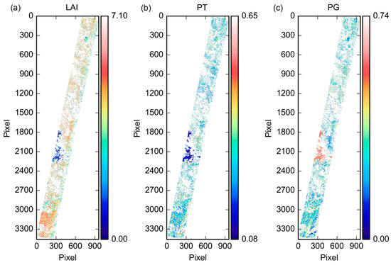
Figure 5.
Spatial patterns of LAI (a) derived using MSR705 and spatial distribution of PT (b) and PG (c) estimated using NASI retrieved from the Hyperion image over the study area at a spatial resolution of 30 m.
The calculated LAI, PT, and PG values were used to determine the M value in the LUTs, and these values were then substituted into the modified spectral down-scaling model to estimate the average leaf reflectance of each pixel of the Hyperion image. The results in Table A5 in Appendix A show that the retrieved average leaf reflectance spectra of the pixels are in good agreement with the measured leaf reflectance spectra at the site level. For sites with low vegetation coverage and complex cover types, such as a water pool contained in the pixel covering the site, the retrieved leaf reflectance spectra are significantly different from the measured leaf reflectance spectra (# 1, 10, 16, 19, 21, 30, 31, and 33). In the other sites, the measured and retrieved reflectance of the leaves are in good agreement; the minimum and maximum adjusted R2 values obtained by the comparison between them in the visible and near-infrared regions are 0.918 and 0.979, with the range of nRMSE as 5.388% to 17.345%, respectively.
3.4. Leaf Water Content Retrieval
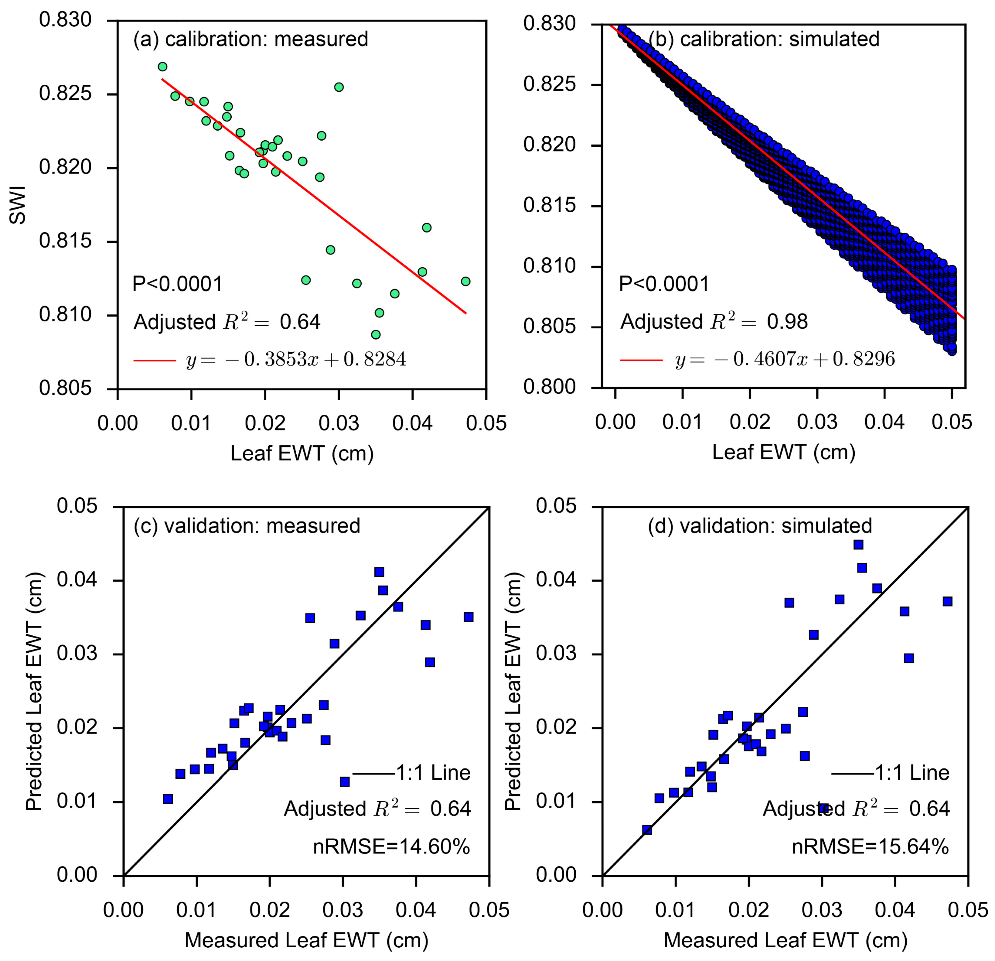
The performance of the two SWI-based EWT models, adapted for Hyperion spectra bands and calibrated using the measured data and the PROSPECT simulated data, respectively, are shown in Figure 6. The performance of the PROSPECT-derived SWI-based model is comparable to the measurement-derived SWI-based model, with the same value of 0.64 (nRMSE = 15.64%), although the measurement-derived SWI-based model has a slightly lower nRMSE value (14.60%). The results indicated the transferability from simulation to in situ data and the generality of the PROSPECT-derived SWI-based EWT retrieval model.
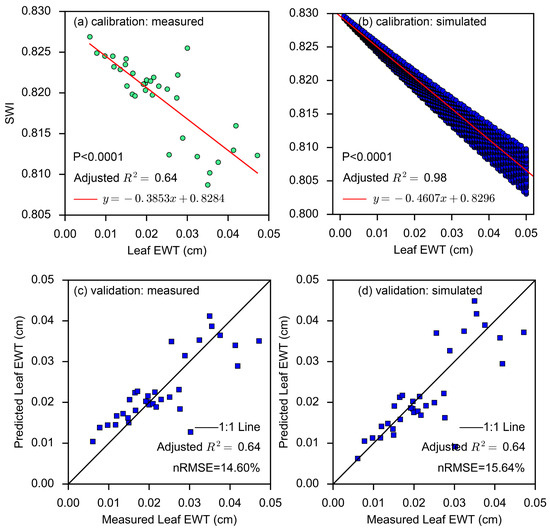
Figure 6.
Correlations between leaf EWT and SWI for the measured data (a) and the simulated data using the PROSPECT model (b). Validation of leaf EWT retrieved using the SWI-based model derived from measured data (c) and the simulated data (d). All leaf reflectance spectra were resampled to Hyperion-equivalent spectra.
We also compared the SWIs-based EWT models and the indices-based EWT models calibrated using the PROSPECT simulated data and validated using the measured data. The resultant and nRMSE values between the estimated and reference EWT are presented in Table 1. The SWI-based EWT model obtained a more accurate estimation than all index-based EWT models, with a nRMSE value of 15.64% and of 0.64 (Table 1). In the specific analysis presented in Figure 6, the data points are distributed around the 1:1 line, suggesting a general alignment between SWI-based model predictions and measured EWT values. However, there is noticeable scatter, particularly at higher EWT values, indicating some variability in the predictions. In the lower EWT range, data points are more densely clustered around the 1:1 line, indicating good agreement between predicted and measured values. At higher EWT values, the scatter increases significantly, and several data points deviate notably from the 1:1 line. This greater dispersion suggests that the model’s accuracy diminishes at higher EWT levels. Overall, it can be inferred that, even without the measured leaf data, the PROSPECT-derived SWI-based EWT retrieval model is a good choice to invert leaf EWT in practice.

Table 1.
The ability of SWI and 6 different spectral indices to retrieve leaf EWT #.
Leaf EWT was mapped using the PROSPECT-derived SWI-based EWT retrieval model, and the leaf reflectance data was inverted from the Hyperion image using a modified spectral down-scaling model (Figure 7a). The average value of the LWC () at the pixel scale obtained by the inversion model is mainly concentrated in 0.02–0.03 g/cm2, which is significantly smaller than the range of EWT of the measured leaves (0–0.05 g/cm2). The reason might be that the ground observation was sampled for limited leaves, and the pixel scale values represented the mean value within a pixel (30 × 30 m). The variation range of pixels will be smaller than that of the sampled leaves.
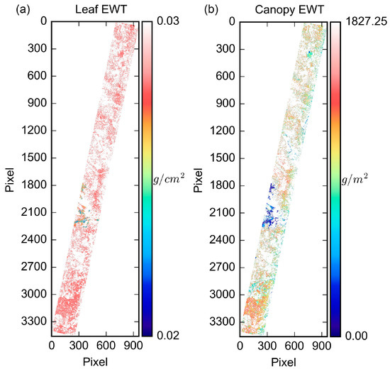
Figure 7.
Spatial distribution of average leaf EWT inverted from coupled down-scaling inversion strategy (a) and canopy water content per unit ground surface area derived based on the LAI image and retrieved average leaf EWT (b). The spatial resolution of the image is 30 × 30 m.
3.5. Canopy Water Content Retrieval and Mapping
Table 2 shows the comparison between the down-scaling inversion strategy and the direct inversion strategy. The R2 values for the direct inversion approach are generally low, with most values falling below 0.2. For the LWC, the highest R2 value is 0.0490 (SANI), indicating a very weak correlation. For the CWC, the highest R2 value is 0.1971 (SASI), which is still a weak correlation.
Table 2.
Correlations of measured leaf and canopy water content with SWI and spectral indices calculated from the Hyperion image using direct and down-scale approaches.
All models using the down-scaling inversion strategy outperformed models using the direct inversion strategy. The highest R2 value for the LWC is 0.0543 (SWI), which is still relatively low but better than the direct inversion approach. For the CWC, the R2 values are notably higher, with SWI achieving the highest value of 0.7869. The SWI-based model (R2 = 0.7869) performed far better than the best indices-based inversion model (SANI, R2 = 0.5424).
There is a scale mismatch problem at the leaf scale, where the leaf-level mean water content is retrieved, and the measured LWC has a large heterogeneity within each pixel, resulting in a very low R2 between the retrieved and measured values. At the canopy scale, the low R2 values in the direct inversion approach highlight the limitations of this method in accounting for the complexity of canopy structures and soil background variability. The down-scale inversion approach, however, accounts for the multiple scattering effects and the structural heterogeneity of the canopy and has validated its effectiveness in capturing water content variations at the canopy level.
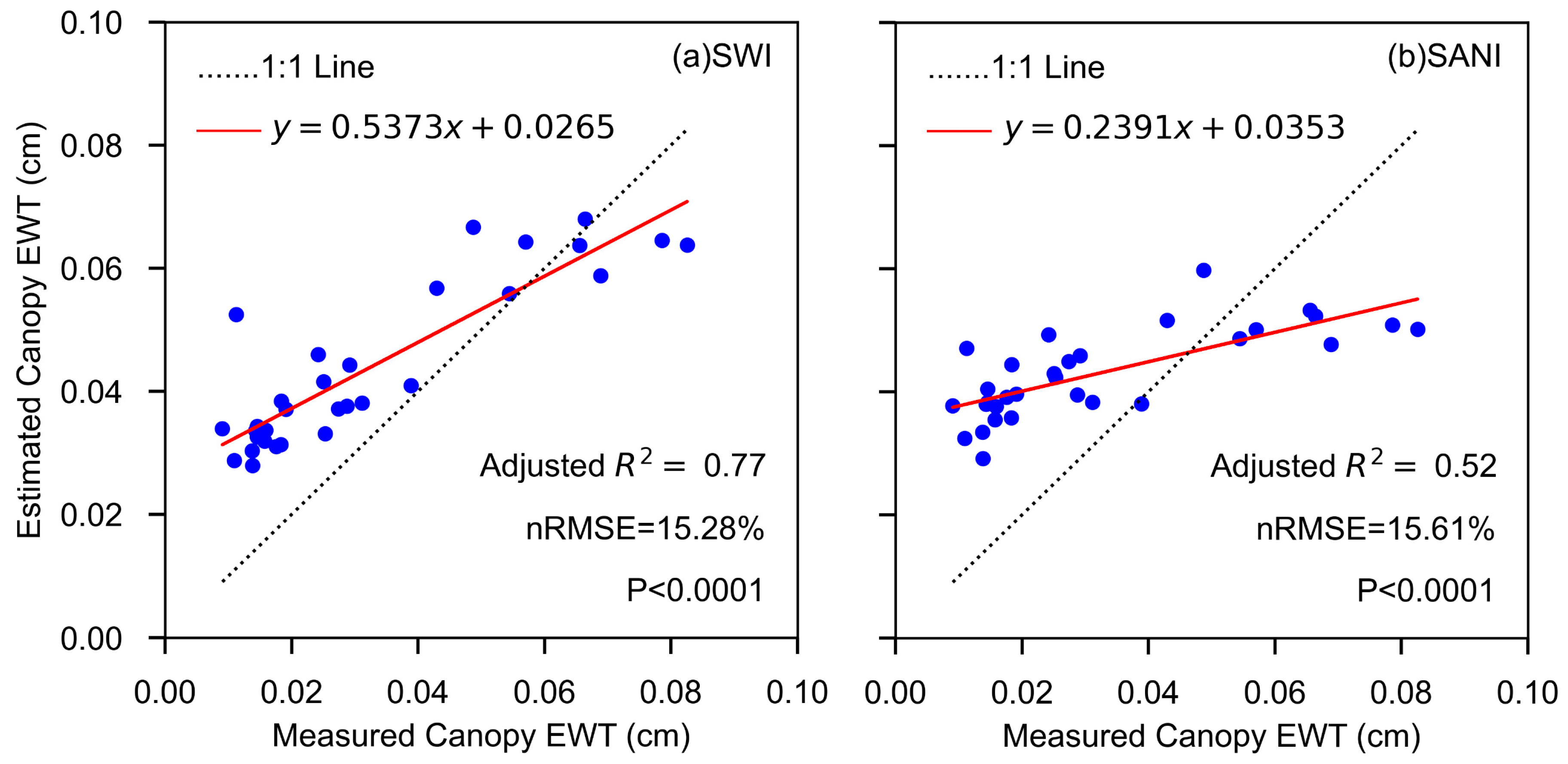
Figure 8 shows the comparisons of the canopy EWT obtained via the down-scaling inversion strategy using (a) the SWI-based and (b) the SANI-based model with ground observations, which was calculated as the product of the ground-measured LWC and LAI. The SWI-based inversion model obtained the most accurate estimation, with a nRMSE value of 15.28% ( = 0.77, NO. = 28) between the inverted CWC and measured data. The nRMSE of the CWC inverted from the SANI-based inversion model against the measured data is 15.61% (with = 0.52).
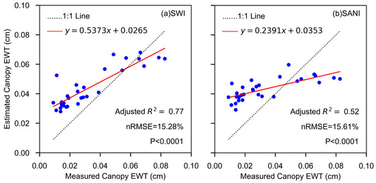
Figure 8.
Comparison of measured CWC against those retrieved from SWI-based (a) and SANI-based (b) coupled models using the down-scaling inversion strategy.
Figure 7b shows the canopy water content (EWTcanopy = × LAI) per unit ground area derived from the leaf EWT map and the LAI map. The value of EWTcanopy maximizes 1827.25 g/m2. The mean value is 1011.14 g/m2, and the standard deviation is 303.13 g/m2. The spatial distribution characteristics of EWTcanopy are influenced by both the and LAI. EWTcanopy is relatively high in the south of the study area.
4. Discussion
4.1. Comparison of Two Inversion Strategies
In order to evaluate the effect of the canopy structure and background on the inverted leaf and CWC, we performed a comparison of the two strategies. The first is the direct inversion strategy, which does not explicitly consider the influence of canopy structure and background and directly uses the canopy reflectance data from the Hyperion image to establish the leaf and CWC estimation models. The second is the down-scaling inversion strategy used in this study, which first inverts leaf spectra and then the leaf and CWCs. Using the direct inversion strategy, the correlations of the SWI index and six spectral indices directly calculated from Hyperion image data with ground-measured leaf and CWC were not significant, with all p values above 0.05 for all indices (Table 2). Using the down-scaling inversion strategy, the correlation between inverted CWC and the ground measurements was significantly improved for all indices. Among the six traditional spectral indices, SANI had the better performance (R2 = 0.5424, p < 0.0001), but SWI proposed by Fang et al. [32] had the best performance (R2 = 0.7869, p < 0.0001). The down-scaling inversion strategy is superior to the direct inversion because the effects of canopy structure and background reflections are well constrained.
4.2. Effect of Canopy Structure and Background
The effect of canopy structure on observed canopy reflectance in this study was quantitatively characterized by PT and PG, and the contributions of the two shaded components and multiple scattering were quantitatively characterized by the multiple scattering factor M. The LUT of M relies on prior knowledge of the LAI, which is the key input information for leaf reflectance extraction and CWC estimation. Fortunately, there are many LAI global products available today, and the quality of these products has been improving [33,34,35,36].
The effect of the ground background reflection is directly considered, and it is a necessary input parameter for the spectral down-scaling model. Ground background reflections can be obtained from field observations, extracted from pure soil pixels on an image, and estimated by querying a soil spectral library. Moreover, there have been studies specifically for the retrieval of soil background from multi-angle remote sensing, which can also provide accurate background reflectance information on a large region [37,38].
4.3. Advantages and Disadvantages of Proposed Models
The proposed models in this study have certain advantages, including being insensitive to the vegetation species, canopy structure, and soil background, and thus being usable in different ecosystems. Another advantage is the transferability of models, which can be calibrated using simulated data and then applied directly to satellite data.
Nevertheless, there are still some limitations that need to be addressed in the future.
The LAI is a key parameter in the proposed models. It affects the CWC estimation in two steps: in the conversion of the leaf to the CWC and in the determination of multiple scattering factor M. In this study, the LAI was estimated using a locally calibrated empirical model. This approach is not applicable at regional and global scales. Therefore, errors in estimated CWC induced by the LAI must be quantified. The improvement of the LAI quality is required for better estimation from satellite data.
The models retrieving leaf and CWC were proposed and tested using hyperspectral satellite data. The availability of hyperspectral satellite data is relatively low in comparison with that of multi-spectral satellite data. Because of the benefits of a regular revisit, rapid update, and large coverage, multi-spectral data can provide important data for real-time, rapid, and large-scale dynamic monitoring of the CWC. The applicability of models proposed in this study for multi-spectral satellite data needs further investigation.
5. Conclusions
This study proposed a novel strategy for retrieving the CWC by coupling a modified spectral down-scaling model and an LWC remote sensing inversion model. The down-scaling inversion strategy considered the influences of the canopy structure and background to improve the inversion accuracy of the CWC. Satellite-ground synchronous observation data were used for validation. Our down-scaling inversion strategy can be used to retrieve the CWC from Hyperion images accurately and outperform the direct inversion strategy based on the widely used spectral index approach. The modified spectral down-scaling model developed in this study efficiently retrieved the leaf reflectance spectra from the canopy spectra of remote sensing imagery. In combination with the leaf-level SWI-based model, the canopy EWT was estimated from remote sensing imagery with improved accuracy. Canopy EWT mapped at 30 m resolution can provide insight into forest growth and ecosystem health, as well as the potential for climate change. The down-scaling inversion strategy would also be useful for improving the inversion accuracy of other vegetation canopy biochemical components.
Author Contributions
M.F.: Conceptualization, Methodology, Software, Writing—original draft, Project administration; X.H.: Software, Validation, Visualization; J.M.C.: Software, Supervision, Writing—review and editing; X.Z.: Validation, Visualization; X.T.: Resources, Funding acquisition; H.L.: Formal analysis, Data curation; M.X.: Investigation; W.J.: Conceptualization, Methodology, Writing—review and editing. All authors have read and agreed to the published version of the manuscript.
Funding
This research was funded by the National Natural Science Foundation of China (41801251, 42201360, 41671343, and 42001302); the “Pioneer” and “Leading Goose” R&D Program of Zhejiang (2024C03226); the China Postdoctoral Science Foundation (2018M642207); and the Key Laboratory of National Geographic Census and Monitoring, Ministry of Natural Resources (2024NGCM06).
Data Availability Statement
The data presented in this study are available on request from the corresponding author.
Acknowledgments
The authors honestly thank Zheng Niu for providing the Yunnan satellite-ground synchronous observation data.
Conflicts of Interest
The authors declare no conflicts of interest.
Appendix A
This appendix includes two figures and five tables.
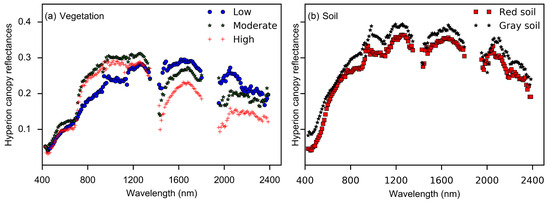
Figure A1.
After preprocessing of the Hyperion image, spectra were compared between (a) vegetation with different crown closures (high, moderate, and low coverage) and (b) soil background with red and gray hues. Data were adapted from Fang et al. [25].
Figure A1.
After preprocessing of the Hyperion image, spectra were compared between (a) vegetation with different crown closures (high, moderate, and low coverage) and (b) soil background with red and gray hues. Data were adapted from Fang et al. [25].


Figure A2.
Correlations of the viewing probabilities of sunlit crown and background (PT and PG) based on the 4-Scale GO model simulations from the Hyperion synthetic data, which includes 10,764 scenes.
Figure A2.
Correlations of the viewing probabilities of sunlit crown and background (PT and PG) based on the 4-Scale GO model simulations from the Hyperion synthetic data, which includes 10,764 scenes.
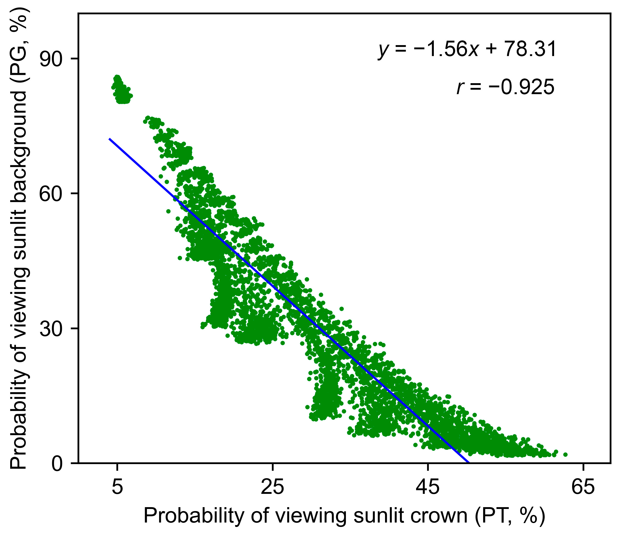
Table A1.
Hyperion includes 242 channels at a 10 nm spectral resolution covering the visible, near-infrared (NIR) and shortwave-infrared (SWIR) ranges, ranging from 400 nm to 2500 nm. The excluded and included Hyperion bands in our study are listed below.
Table A1.
Hyperion includes 242 channels at a 10 nm spectral resolution covering the visible, near-infrared (NIR) and shortwave-infrared (SWIR) ranges, ranging from 400 nm to 2500 nm. The excluded and included Hyperion bands in our study are listed below.
| Excluded Bands | Wavelength (nm) | Exclusion Criteria | Included Bands | Wavelength (nm) |
|---|---|---|---|---|
| VNIR 1–7 | 355–416 | Uncalibrated | VNIR 8–57 | 426–926 |
| VNIR 58–70 | 936–1058 | Uncalibrated | SWIR 79–120 | 933–1346 |
| SWIR 71–76 | 852–902 | Uncalibrated | SWIR 128–165 | 1427–1810 |
| SWIR 77–78 | 912–923 | Overlap and high noise | SWIR 180–223 | 1942–2385 |
| SWIR 121–127 | 1356–1417 | Water vapor interference | ||
| SWIR 166–179 | 1820–1931 | Water vapor interference | ||
| SWIR 224 | 2395 | Water vapor interference | ||
| SWIR 225–242 | 2405–2577 | Uncalibrated | ||
| Total: 68 | Total: 174 |
Note: VNIR (visible and near-infrared range); SWIR (shortwave infrared range).
Table A2.
Input parameter values for PROSPECT and 4-Scale GO models are used to simulate the Hyperion pixel-scale canopy reflectance spectra, adapted from Fang et al. [25].
Table A2.
Input parameter values for PROSPECT and 4-Scale GO models are used to simulate the Hyperion pixel-scale canopy reflectance spectra, adapted from Fang et al. [25].
| Model | Input Parameter | Unit | Values |
|---|---|---|---|
| PROSPECT | EWT | cm or g/cm2 | 0.005–0.055 (step = 0.01) |
| Cab | μg/cm2 | 5–95 (step = 30) | |
| Cm | g/cm2 | 0.002–0.038 (step = 0.012) | |
| N | 1–3.5 (step = 0.5) | ||
| 4-Scale GO model | Tree shape | Sphere/Ellipsoid | |
| Stick height | m | 4–18 (step = 7) | |
| Crown height | m | 1.4–7 (step = 2.8) | |
| Radius of crown | m | 0.6–2 (step = 0.7) | |
| Clumping index | 0.9 | ||
| Needle-to-shoot area ratio | 1 | ||
| Soil background | Normal, wet, dry | ||
| Pixel area | m2 | 30 × 30 | |
| Number of trees per ha | 1000–6000 (step = 2500) | ||
| Leaf area index | 0.4–7.3 (step = 0.15) | ||
| Solar zenith angle | degree | 31–36 (step = 0.2) |
Due to the Hyperion observation utilizing zenith observing, the view zenith angle and relative azimuthal angle between the sensor and Sun are the constant as zero (View zenith angle = 0, Relative azimuthal angle = 0).
Table A3.
Statistics for the comparison of canopy reflectance spectra simulated by the 4-Scale GO model with those retrieved from the Hyperion image at different sampling sites.
Table A3.
Statistics for the comparison of canopy reflectance spectra simulated by the 4-Scale GO model with those retrieved from the Hyperion image at different sampling sites.
| NO. | nRMSE (%) | NO. | nRMSE (%) | ||
|---|---|---|---|---|---|
| 1 | 0.947 | 11.124 | 20 | 0.973 | 5.961 |
| 2 | 0.986 | 3.686 | 21 | 0.949 | 6.535 |
| 3 | 0.979 | 4.203 | 22 | 0.981 | 4.280 |
| 4 | 0.976 | 4.522 | 23 | 0.976 | 4.731 |
| 5 | 0.974 | 5.209 | 24 | 0.984 | 4.917 |
| 6 | 0.978 | 4.654 | 25 | 0.982 | 4.294 |
| 7 | 0.983 | 4.228 | 26 | 0.985 | 3.903 |
| 8 | 0.974 | 4.863 | 27 | 0.982 | 4.407 |
| 9 | 0.985 | 3.858 | 28 | 0.975 | 5.109 |
| 10 | 0.951 | 7.225 | 29 | 0.948 | 13.292 |
| 11 | 0.983 | 4.044 | 30 | 0.955 | 6.651 |
| 12 | 0.973 | 6.280 | 31 | 0.972 | 4.794 |
| 14 | 0.987 | 3.406 | 32 | 0.984 | 4.069 |
| 16 | 0.955 | 6.311 | 33 | 0.974 | 5.423 |
| 17 | 0.989 | 3.268 | 34 | 0.975 | 4.848 |
| 18 | 0.969 | 5.785 | 35 | 0.975 | 4.860 |
| 19 | 0.970 | 5.024 |
Table A4.
The example of a lookup table for determining the spectral multiple scattering factor (M) according to LAI, PT and PG.
Table A4.
The example of a lookup table for determining the spectral multiple scattering factor (M) according to LAI, PT and PG.
| Wavelength (nm) | LAI = 0.8 | |||
|---|---|---|---|---|
| PT = 23.78% | PG = 48.56% | PT = 24.82% | PG = 50.50% | |
| 468 | 1.0282 | 1.0166 | ||
| 478 | 1.0304 | 1.0194 | ||
| 488 | 1.0332 | 1.0212 | ||
| 498 | 1.0369 | 1.0243 | ||
| 508 | 1.0434 | 1.0286 | ||
| 1003 | 1.5996 | 1.3636 | ||
| 1013 | 1.6176 | 1.3679 | ||
| 1023 | 1.6238 | 1.3751 | ||
| 1033 | 1.6260 | 1.3833 | ||
| 1044 | 1.6373 | 1.3871 | ||
| 1588 | 1.5338 | 1.4436 | ||
| 1599 | 1.5436 | 1.4530 | ||
| Wavelength (nm) | LAI = 5 | |||
| PT = 16.82% | PG = 36.33% | PT = 44.79% | PG = 1.71% | |
| 468 | 1.0185 | 1.0034 | ||
| 478 | 1.0197 | 1.0036 | ||
| 488 | 1.0214 | 1.0038 | ||
| 498 | 1.0237 | 1.0042 | ||
| 508 | 1.0282 | 1.0052 | ||
| 1003 | 1.9835 | 1.2837 | ||
| 1013 | 2.0104 | 1.2923 | ||
| 1023 | 2.0271 | 1.2979 | ||
| 1033 | 2.0468 | 1.3089 | ||
| 1044 | 2.0729 | 1.3198 | ||
| 1588 | 1.7686 | 1.0881 | ||
| 1599 | 1.7948 | 1.0921 | ||
Table A5.
Statistics for the comparison of leaf reflectance inverted from the Hyperion image using the modified spectral down-scaling model with measurements at different sampling sites.
Table A5.
Statistics for the comparison of leaf reflectance inverted from the Hyperion image using the modified spectral down-scaling model with measurements at different sampling sites.
| NO. | nRMSE (%) | NO. | nRMSE (%) | ||
|---|---|---|---|---|---|
| 1 | 0.029 | 45.377 | 20 | 0.959 | 8.917 |
| 2 | 0.959 | 7.444 | 21 | 0.388 | 32.424 |
| 3 | 0.947 | 8.065 | 22 | 0.939 | 9.944 |
| 4 | 0.961 | 7.874 | 23 | 0.957 | 8.855 |
| 5 | 0.941 | 11.867 | 24 | 0.979 | 6.987 |
| 6 | 0.952 | 8.335 | 25 | 0.961 | 7.636 |
| 7 | 0.973 | 6.394 | 26 | 0.967 | 7.209 |
| 8 | 0.922 | 10.611 | 27 | 0.958 | 7.888 |
| 9 | 0.950 | 8.739 | 28 | 0.948 | 9.005 |
| 10 | 0.851 | 14.192 | 29 | 0.921 | 17.345 |
| 11 | 0.935 | 9.790 | 30 | 0.122 | 44.586 |
| 12 | 0.963 | 8.716 | 31 | 0.675 | 24.454 |
| 14 | 0.974 | 6.394 | 32 | 0.979 | 5.388 |
| 16 | 0.808 | 17.736 | 33 | 0.807 | 17.178 |
| 17 | 0.963 | 8.036 | 34 | 0.930 | 9.868 |
| 18 | 0.952 | 8.673 | 35 | 0.918 | 11.156 |
| 19 | 0.848 | 15.213 |
References
- Bueso, D.; Piles, M.; Ciais, P.; Wigneron, J.P.; Moreno-Martinez, A.; Camps-Valls, G. Soil and vegetation water content identify the main terrestrial ecosystem changes. Natl. Sci. Rev. 2023, 10, nwad026. [Google Scholar] [CrossRef] [PubMed]
- Konings, A.G.; Saatchi, S.S.; Frankenberg, C.; Keller, M.; Leshyk, V.; Anderegg, W.R.L.; Humphrey, V.; Matheny, A.M.; Trugman, A.; Sack, L.; et al. Detecting forest response to droughts with global observations of vegetation water content. Glob. Chang. Biol. 2021, 27, 6005–6024. [Google Scholar] [CrossRef] [PubMed]
- Bernardino, P.N.; Oliveira, R.S.; Van Meerbeek, K.; Hirota, M.; Furtado, M.N.; Sanches, I.A.; Somers, B. Estimating vegetation water content from Sentinel-1 C-band SAR data over savanna and grassland ecosystems. Environ. Res. Lett. 2024, 19, 034019. [Google Scholar] [CrossRef]
- Ullah, S.; Skidmore, A.K.; Groen, T.A.; Schlerf, M. Evaluation of three proposed indices for the retrieval of leaf water content from the mid-wave infrared (2–6 μm) spectra. Agric. For. Meteorol. 2013, 171–172, 65–71. [Google Scholar] [CrossRef]
- Ullah, S.; Skidmore, A.K.; Naeem, M.; Schlerf, M. An accurate retrieval of leaf water content from mid to thermal infrared spectra using continuous wavelet analysis. Sci. Total Environ. 2012, 437, 145–152. [Google Scholar] [CrossRef]
- Zhang, F.; Zhou, G. Estimation of vegetation water content using hyperspectral vegetation indices: A comparison of crop water indicators in response to water stress treatments for summer maize. BMC Ecol. 2019, 19, 18. [Google Scholar] [CrossRef]
- Gao, Y.; Walker, J.P.; Allahmoradi, M.; Monerris, A.; Ryu, D.; Jackson, T.J. Optical sensing of vegetation water content: A synthesis study. IEEE J. Sel. Top. Appl. Earth Obs. Remote Sens. 2015, 8, 1456–1464. [Google Scholar] [CrossRef]
- Zhang, C.; Pattey, E.; Liu, J.; Cai, H.; Shang, J.; Dong, T. Retrieving leaf and canopy water content of winter wheat using vegetation water indices. IEEE J. Sel. Top. Appl. Earth Obs. Remote Sens. 2018, 11, 112–126. [Google Scholar] [CrossRef]
- Rouse, J.W., Jr.; Haas, R.; Schell, J.; Deering, D. Monitoring vegetation systems in the Great Plains with ERTS. NASA Spec. Publ. 1974, 351, 309–317. [Google Scholar]
- Gao, B.-C. NDWI—A normalized difference water index for remote sensing of vegetation liquid water from space. Remote Sens. Environ. 1996, 58, 257–266. [Google Scholar] [CrossRef]
- Jackson, T.J.; Chen, D.; Cosh, M.; Li, F.; Anderson, M.; Walthall, C.; Doriaswamy, P.; Hunt, E.R. Vegetation water content mapping using Landsat data derived normalized difference water index for corn and soybeans. Remote Sens. Environ. 2004, 92, 475–482. [Google Scholar] [CrossRef]
- Chai, L.; Jiang, H.; Crow, W.T.; Liu, S.; Zhao, S.; Liu, J.; Yang, S. Estimating corn canopy water content from normalized difference water index (NDWI): An optimized NDWI-based scheme and its feasibility for retrieving corn VWC. IEEE Trans. Geosci. Remote Sens. 2021, 59, 8168–8181. [Google Scholar] [CrossRef]
- Khanna, S.; Palacios-Orueta, A.; Whiting, M.L.; Ustin, S.L.; Riaño, D.; Litago, J. Development of angle indexes for soil moisture estimation, dry matter detection and land-cover discrimination. Remote Sens. Environ. 2007, 109, 154–165. [Google Scholar] [CrossRef]
- Ullah, S.; Skidmore, A.K.; Ramoelo, A.; Groen, T.A.; Naeem, M.; Ali, A. Retrieval of leaf water content spanning the visible to thermal infrared spectra. ISPRS J. Photogramm. Remote Sens. 2014, 93, 56–64. [Google Scholar] [CrossRef]
- Hardisky, M.; Klemas, V.; Smart, M. The influence of soil salinity, growth form, and leaf moisture on the spectral radiance of Spartina alterniflora Canopies. Photogramm. Eng. Remote Sens. 1983, 49, 77–83. [Google Scholar]
- Gao, B.-C.; Goetz, A.F. Retrieval of equivalent water thickness and information related to biochemical components of vegetation canopies from AVIRIS data. Remote Sens. Environ. 1995, 52, 155–162. [Google Scholar] [CrossRef]
- Gao, B.C.; Goetz, A.F. Column atmospheric water vapor and vegetation liquid water retrievals from airborne imaging spectrometer data. J. Geophys. Res. Atmos. 1990, 95, 3549–3564. [Google Scholar] [CrossRef]
- Zarco-Tejada, P.J.; Rueda, C.A.; Ustin, S.L. Water content estimation in vegetation with MODIS reflectance data and model inversion methods. Remote Sens. Environ. 2003, 85, 109–124. [Google Scholar] [CrossRef]
- Riaño, D.; Vaughan, P.; Chuvieco, E.; Zarco-Tejada, P.J.; Ustin, S.L. Estimation of fuel moisture content by inversion of radiative transfer models to simulate equivalent water thickness and dry matter content: Analysis at leaf and canopy level. IEEE Trans. Geosci. Remote Sens. 2005, 43, 819–826. [Google Scholar] [CrossRef]
- Cheng, T.; Riaño, D.; Ustin, S.L. Detecting diurnal and seasonal variation in canopy water content of nut tree orchards from airborne imaging spectroscopy data using continuous wavelet analysis. Remote Sens. Environ. 2014, 143, 39–53. [Google Scholar] [CrossRef]
- Casas, A.; Riaño, D.; Ustin, S.; Dennison, P.; Salas, J. Estimation of water-related biochemical and biophysical vegetation properties using multitemporal airborne hyperspectral data and its comparison to MODIS spectral response. Remote Sens. Environ. 2014, 148, 28–41. [Google Scholar] [CrossRef]
- Wang, L.; Qu, J.J. NMDI: A normalized multi-band drought index for monitoring soil and vegetation moisture with satellite remote sensing. Geophys. Res. Lett. 2007, 34, L20405. [Google Scholar] [CrossRef]
- Yilmaz, M.T.; Hunt, E.R.; Jackson, T.J. Remote sensing of vegetation water content from equivalent water thickness using satellite imagery. Remote Sens. Environ. 2008, 112, 2514–2522. [Google Scholar] [CrossRef]
- Zhang, Y.; Chen, J.M.; Miller, J.R.; Noland, T.L. Leaf chlorophyll content retrieval from airborne hyperspectral remote sensing imagery. Remote Sens. Environ. 2008, 112, 3234–3247. [Google Scholar] [CrossRef]
- Fang, M.; Ju, W.; Chen, J.M.; Fan, W.; He, W.; Qiu, F.; Hu, X.; Li, J. A Normalized Spectral Angle Index for Estimating the Probability of Viewing Sunlit Leaves From Satellite Data. IEEE Trans. Geosci. Remote Sens. 2023, 61, 4401519. [Google Scholar] [CrossRef]
- Wu, C.; Han, X.; Niu, Z.; Dong, J. An evaluation of EO-1 hyperspectral Hyperion data for chlorophyll content and leaf area index estimation. Int. J. Remote Sens. 2010, 31, 1079–1086. [Google Scholar] [CrossRef]
- Sun, Z.; Bu, Z.; Lu, S.; Omasa, K. A general algorithm of leaf chlorophyll content estimation for a wide range of plant species. IEEE Trans. Geosci. Remote Sens. 2022, 60, 4406814. [Google Scholar] [CrossRef]
- Pisek, J.; Ryu, Y.; Sprintsin, M.; He, L.; Oliphant, A.J.; Korhonen, L.; Kuusk, J.; Kuusk, A.; Bergstrom, R.; Verrelst, J.; et al. Retrieving vegetation clumping index from Multi-angle Imaging SpectroRadiometer (MISR) data at 275m resolution. Remote Sens. Environ. 2013, 138, 126–133. [Google Scholar] [CrossRef]
- Chen, J.M.; Leblanc, S.G. A four-scale bidirectional reflectance model based on canopy architecture. IEEE Trans. Geosci. Remote Sens. 1997, 35, 1316–1337. [Google Scholar] [CrossRef]
- Fan, W.; Li, J.; Liu, Q. GOST2: The Improvement of the Canopy Reflectance Model GOST in Separating the Sunlit and Shaded Leaves. IEEE J. Sel. Top. Appl. Earth Obs. Remote Sens. 2015, 8, 1423–1431. [Google Scholar] [CrossRef]
- Widlowski, J.L.; Pinty, B.; Gobron, N.; Verstraete, M.M.; Diner, D.J.; Davis, A.B. Canopy Structure Parameters Derived from Multi-Angular Remote Sensing Data for Terrestrial Carbon Studies. Clim. Chang. 2004, 67, 403–415. [Google Scholar] [CrossRef]
- Fang, M.; Ju, W.; Zhan, W.; Cheng, T.; Qiu, F.; Wang, J. A new spectral similarity water index for the estimation of leaf water content from hyperspectral data of leaves. Remote Sens. Environ. 2017, 196, 13–27. [Google Scholar] [CrossRef]
- Fang, H.; Wei, S.; Jiang, C.; Scipal, K. Theoretical uncertainty analysis of global MODIS, CYCLOPES, and GLOBCARBON LAI products using a triple collocation method. Remote Sens. Environ. 2012, 124, 610–621. [Google Scholar] [CrossRef]
- Fang, H.; Baret, F.; Plummer, S.; Schaepman-Strub, G. An overview of global leaf area index (LAI): Methods, products, validation, and applications. Rev. Geophys. 2019, 57, 739–799. [Google Scholar] [CrossRef]
- Xu, B.; Li, J.; Park, T.; Liu, Q.; Zeng, Y.; Yin, G.; Zhao, J.; Fan, W.; Yang, L.; Knyazikhin, Y.; et al. An integrated method for validating long-term leaf area index products using global networks of site-based measurements. Remote Sens. Environ. 2018, 209, 134–151. [Google Scholar] [CrossRef]
- Baret, F.; Hagolle, O.; Geiger, B.; Bicheron, P.; Miras, B.; Huc, M.; Berthelot, B.; Niño, F.; Weiss, M.; Samain, O. LAI, fAPAR and fCover CYCLOPES global products derived from VEGETATION: Part 1: Principles of the algorithm. Remote Sens. Environ. 2007, 110, 275–286. [Google Scholar] [CrossRef]
- Pisek, J.; Rautiainen, M.; Heiskanen, J.; Mõttus, M. Retrieval of seasonal dynamics of forest understory reflectance in a Northern European boreal forest from MODIS BRDF data. Remote Sens. Environ. 2012, 117, 464–468. [Google Scholar] [CrossRef]
- Canisius, F.; Chen, J.M. Retrieving forest background reflectance in a boreal region from Multi-angle Imaging SpectroRadiometer (MISR) data. Remote Sens. Environ. 2007, 107, 312–321. [Google Scholar] [CrossRef]


Disclaimer/Publisher’s Note: The statements, opinions and data contained in all publications are solely those of the individual author(s) and contributor(s) and not of MDPI and/or the editor(s). MDPI and/or the editor(s) disclaim responsibility for any injury to people or property resulting from any ideas, methods, instructions or products referred to in the content. |
© 2024 by the authors. Licensee MDPI, Basel, Switzerland. This article is an open access article distributed under the terms and conditions of the Creative Commons Attribution (CC BY) license (https://creativecommons.org/licenses/by/4.0/).