Article

Temporal Variations in Methane Emissions from a Restored Mangrove Ecosystem in Southern China

by
Pengpeng Tian
1,
Xianglan Li
1,*,
Zhe Xu
1,
Liangxu Wu
1,
Yuting Huang
1,
Zhao Zhang
2,
Mengna Chen
2,
Shumin Zhang
2,
Houcai Cai
3,
Minghai Xu
4 and
Wei Chen
4
1
State Key Laboratory of Remote Sensing, College of Global Change and Earth System Science, Faculty of Geographical Science, Beijing Normal University, Beijing 100875, China
2
Wenzhou Marine Center, Ministry of Natural Resources, Wenzhou 325011, China
3
Administration of Nanji Archipelago National Marine Nature Reserve, Wenzhou 325408, China
4
Pingyang Natural Resources and Planning Bureau, Wenzhou 325400, China
*
Author to whom correspondence should be addressed.
Forests 2024, 15(9), 1487; https://doi.org/10.3390/f15091487 (registering DOI)
Submission received: 5 August 2024 / Revised: 21 August 2024 / Accepted: 23 August 2024 / Published: 24 August 2024
(This article belongs to the Section Forest Ecology and Management)

Abstract

:
The role of coastal mangrove wetlands in sequestering atmospheric carbon dioxide has been increasingly investigated in recent years. While studies have shown that mangroves are weak sources of methane (CH4) emissions, measurements of CH4 fluxes from these ecosystems remain scarce. In this study, we examined the temporal variation and biophysical drivers of ecosystem-scale CH4 fluxes in China’s northernmost mangrove ecosystem based on eddy covariance measurements obtained over a 3-year period. In this mangrove, the annual CH4 emissions ranged from 6.15 to 9.07 g C m−2 year−1. The daily CH4 flux reached a peak of over 0.07 g C m−2 day−1 during the summer, while the winter CH4 flux was negligible. Latent heat, soil temperature, photosynthetically active radiation, and tide water level were the primary factors controlling CH4 emissions. This study not only elucidates the mechanisms influencing CH4 emissions from mangroves, strengthening the understanding of these processes but also provides a valuable benchmark dataset to validate the model-derived carbon budget estimates for these ecosystems.

1. Introduction

Coastal wetlands such as mangroves, seagrass meadows, and salt marshes are recognized as critical components of what is termed blue carbon, due to their ability to capture and store carbon (C) [1,2]. Among these, mangroves have increasingly been acknowledged as a potent natural C sink, capable of trapping large quantities of carbon [3,4]. These ecosystems act as substantial carbon reservoirs worldwide, storing an estimated 3.7–6.2 Pg C [5]. Despite covering less than 0.1% of the world’s continental area, mangrove forests are highly efficient in sequestering carbon dioxide (CO2) [6,7], with their contribution to carbon sequestration significantly affecting the global carbon budget and assisting in climate change mitigation [8]. Policy initiatives for mangrove conservation and restoration have been widely advocated as a nature-based approach to address climate change and both preserve and enhance blue carbon storage [9,10,11]. However, the anoxic conditions in mangrove sediments also favor the production of other greenhouse gases such as methane (CH4) [12], which is the second largest contributor to the human-induced greenhouse effect after CO2 [13].
The substantial carbon sequestration in mangroves is accompanied by CH4 emissions [14,15]. Mangroves are weak sources of CH4, with an annual flux of 0.05–41.50 g C m−2 [16,17]. The global warming potential of CH4 is approximately 27.9 times that of CO2 over a 100-year period and 81.2 times over a 20-year period [18,19]. These emissions could offset the cooling effect of CO2 uptake by approximately 20%–50% over time horizons of 20 and 100 years [8,15]. Despite being relatively low, CH4 emissions should be considered in blue carbon assessments of mangrove ecosystems [20], as their inclusion would increase the global marine CH4 budget by nearly 50% [12]. However, CH4 emissions from mangroves have not received much attention to date, as saline coastal wetlands (which include mangroves) are usually considered negligible CH4 sources [10]. In mangrove ecosystems, changes in CH4 between the atmosphere and biosphere are primarily driven by methanogens [21,22,23]. As observed in other tropical forests, in mangroves these processes are greatly influenced by climate factors such as temperature and precipitation [24,25,26]. For example, based on a 3-year period of continuous measurements conducted in mangroves located in subtropical estuaries, the analysis revealed that CH4 emissions from these ecosystems were significant, and soil temperature and salinity were the main factors controlling the CH4 flux [15].
The eddy covariance (EC) technique has been extensively employed to monitor long-term, near-continuous exchanges of carbon between the atmosphere and biosphere in diverse ecosystems [27]. Multi-year measurements of CH4 fluxes are essential for better understanding their patterns in mangroves, thereby enhancing the accuracy of CH4 budget assessments [15]. In recent years, the EC technique has become a standard tool for measuring greenhouse gas fluxes across different ecosystems [28,29,30]. Despite more than 200 EC sites globally conducting regular CH4 flux measurements [17], only five currently provide data specifically for mangrove ecosystems [4,8,15,31,32]. Furthermore, previous studies have mostly focused on regions between 20° N and 26° N, with a lack of research at higher latitudes.
The annual CH4 emissions recorded in these regions using the EC technique showed considerable variation, ranging from 3.1 to 40.15 g C m−2 year−1, highlighting substantial regional differences [32,33]. In this study, EC measurements of CH4 fluxes were conducted in a restored mangrove forest in Zhejiang Province between 2020 and 2022. The monitoring site was located in an area corresponding to the northernmost distribution of mangroves in China, aiming to provide an important reference dataset and theoretical support for calculating the blue carbon balance. The primary goals were to (1) characterize the temporal variations in CH4 fluxes in the northernmost restored mangrove forest in China during 2020–2022, capturing both seasonal and interannual changes, and (2) explore the key environmental drivers that influence these CH4 fluxes, identifying the specific factors and their relative contributions.

2. Materials and Methods

2.1. Study Site

This study was conducted in a mangrove restoration region situated along the estuary of the Aojiang River in Wenzhou, Zhejiang Province, southern China (27°34′58″ N, 120°34′13″ E, Figure 1). The mangrove restoration area covered roughly 11 hm2, consisting of two sections that were rehabilitated in 2014 and 2018. The restoration primarily involved Kandelia obovata, with a planting arrangement spaced at 1 m × 1 m. This location corresponds to the northernmost boundary of China’s mangrove distribution and is one of the earliest sites used for mangrove transplantation, making it a special area for studying the blue carbon sink potential. The region is characterized by a subtropical marine monsoon climate with warm and humid conditions all year round. Between 2020 and 2022, the mean annual temperature was 20.4 °C, with an average yearly precipitation of 1588 mm. Zou et al. [34] found that the sediment at the Aojiang restored mangrove exhibited a consistently alkaline pH, averaging 8.01 ± 0.12, with minimal variation throughout the site. The average soil organic carbon content across different layers varied between 6.82 and 7.86 g kg−1 [34]. Additionally, the soil’s electrical conductivity and total dissolved solids concentrations were recorded between 3.86 and 4.07 ms cm−1 and 10.85 and 11.33 g kg−1, respectively [34].

2.2. EC Flux and Meteorological Measurements

The EC system was installed on a 4 m tower positioned at the center of the restoration area (Figure 1). The molar density of CH4 was measured using open-path infrared gas analyzers (LI-7700, LI-COR, Inc., Lincoln, NE, USA) that had been installed in 2019. These were also used to continuously monitor the turbulent fluxes of CO2 and CH4 as well as several environmental parameters, including latent heat (LE), sensible heat (H), horizontal wind speed (WS), wind direction (WD), and barometric pressure (PA). To ensure the gas analyzers maintained strong signal quality, their upper and lower windows were cleaned two to three times weekly, either manually on-site or remotely online. The Biomet system (7900-101, LI-COR Inc.) was used to continuously measure a number of additional environmental parameters from 2020 to 2022. These variables included air temperature (Tair), relative humidity (RH), precipitation, and photosynthetically active radiation (PAR), and were measured at a height of 4 m. Measurements for soil temperature (Tsoil) and soil water content (SWC) were taken at a depth of 5 cm. The vapor pressure difference (VPD) was derived from the Tair and RH measurements [35]. Data were recorded every 30 min and averaged using a data recorder (7900-120 Sutron, LI-COR Inc.). Tidal water level (TWL) data were acquired from the Aojiang tide level station, located 5.50 km upstream of the Aojiang River estuary.

2.3. Processing of Flux Data and Gap-Filling

The raw 10 Hz EC data were processed using EddyPro (Version 7.0.9, LI-COR) to produce fluxes averaged over 30 min intervals. The data processing included steps like double rotation [36], covariance maximization [37], analytical corrections for high-pass and low-pass filtering, as well as spectral attenuations [38]. Additional adjustments were made for air density [39] and flux distortions caused by heat, water vapor transfer, steady-state conditions, and turbulence [40]. After processing in EddyPro, additional quality control was applied by excluding CH4 flux data labeled as “2”. The friction velocity (u*) threshold was determined according to the method described by Papale et al. [41] to classify low-turbulence conditions. Fluxes were discarded when u* fell below the thresholds of 0.149, 0.155, and 0.117 m s⁻1 for the years 2020, 2021, and 2022, respectively. Anomalous data (i.e., values that were 1.96 times higher than the standard deviation of five continuous values, including itself) and data collected during rainy periods were discarded [15]. The analysis included CH4 flux data only when the signal strength was above 10, indicating a reliable optical path condition [15]. Overall, 40% of the CH4 flux data were retained.
Based on the eddy covariance method, CH4 flux commonly includes gaps due to unsuitable atmospheric conditions and system failures [27]. CH4 flux data were gap-filled using the random forest (RF) algorithm with an R package, which outperformed other techniques at all sites [27]. The method first assessed the importance of biological drivers for CH4 and then used these insights to train the model and fill the gaps in the CH4 flux.

2.4. Random Forest Models

CH4 emissions are governed by a multitude of nonlinear biogeochemical processes [8,33,42,43]. To tackle the challenges arising from nonlinearity and collinearity among explanatory variables, we used RF models, which allowed us to analyze the relative importance between daily CH4 flux and different environmental drivers. We also conducted a stepwise regression analysis to comparatively evaluate the importance of these drivers. Both the RF model and regression models utilized the original measured flux data.
RF models fit an extensive ensemble of regression trees to bootstrapped samples of a response variable and average the outputs to produce a simulated response. This method, which is used for regression analysis and evaluating the importance of variables, has been widely applied in ecological studies focusing on model predictions and the analysis of environmental drivers [44]. RF models have been frequently employed in mangrove studies to analyze environmental drivers and forecast variations in carbon fluxes [8,15]. We conducted 200 iterations of RF estimation, reporting the mean values and standard deviations to reduce model uncertainty. This analysis was executed using the scikit-learn library in Python v3.10.7 [45].

2.5. Statistical Analysis

To explore the relationships between both daily and monthly CH4 flux and various abiotic variables, Pearson correlation analysis was employed to compute the correlation coefficients. Specifically, the variables included in the models were Tair, Tsoil, LE, H, RH, VPD, PAR, SWC, precipitation, and TWL. The Pearson correlation coefficients were calculated and visualized using the Correlation Plot APPs of Origin software (version 2021, OriginLab). The areas with different colors in the heat maps indicated the positivity or negativity of correlations between variables.
Path analysis, which builds upon multiple regression techniques, is a valuable tool for examining variable relationships [46,47]. For this study, we employed the piecewise structural equation modeling (piecewise SEM) package in R (Version 2.3.0) to conduct the analysis [48]. The design of the path analysis was informed by existing knowledge of the causal links between CH4 emissions and environmental variables.

3. Results

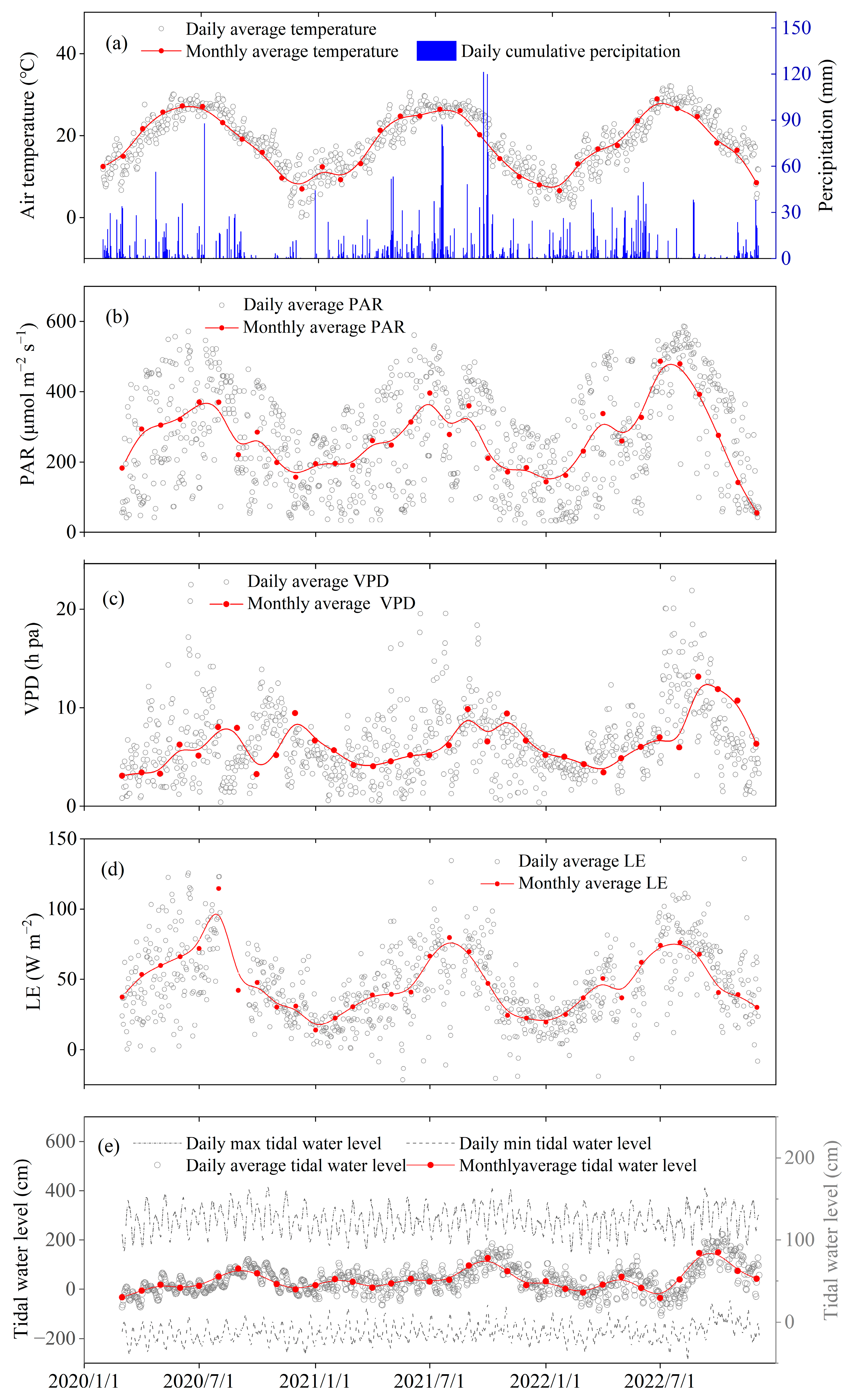
3.1. Environmental Conditions in the Restored Mangrove Ecosystem during 2020–2022

Meteorological data from the study site revealed distinct seasonal patterns typical of a subtropical monsoonal climate, with summers characterized by heat and rainfall, and winters by cold and dryness (Figure 2). The average monthly Tair during summer was 25.63 °C, while in winter it was 15.25 °C. The mean annual air temperature fluctuated between 19.72 °C and 20.85 °C, with only minor variations (Figure 2a). The mean monthly Tsoil ranged from 11.0 to 28.0 °C during the 2020–2022 period. On the monthly scale, Tsoil varied less than Tair. Significant variation in annual precipitation was observed across the three years examined, with totals of 1204 mm, 2116 mm, and 1442 mm for 2020, 2021, and 2022, respectively (Figure 2a). Daily PAR showed a unimodal pattern during 2020–2022, with values ranging from 2.39 to 676 μmol m–2 s–1 and peaking in August (Figure 2b). The average monthly VPD varied between 3.09 and 13.15 hPa, with a daily peak of 2.31 kPa recorded in July 2022 (Figure 2c). Daily LE showed clear seasonality, with values ranging from −14.47 to 125.60 W m−2 (Figure 2d). The daily LE values also showed seasonal variations. The tidal water level (TWL) exhibited distinct variations at the seasonal scale but not at the interannual scale (Figure 2e). Its daily mean values ranged from 8.34 to 107 cm.

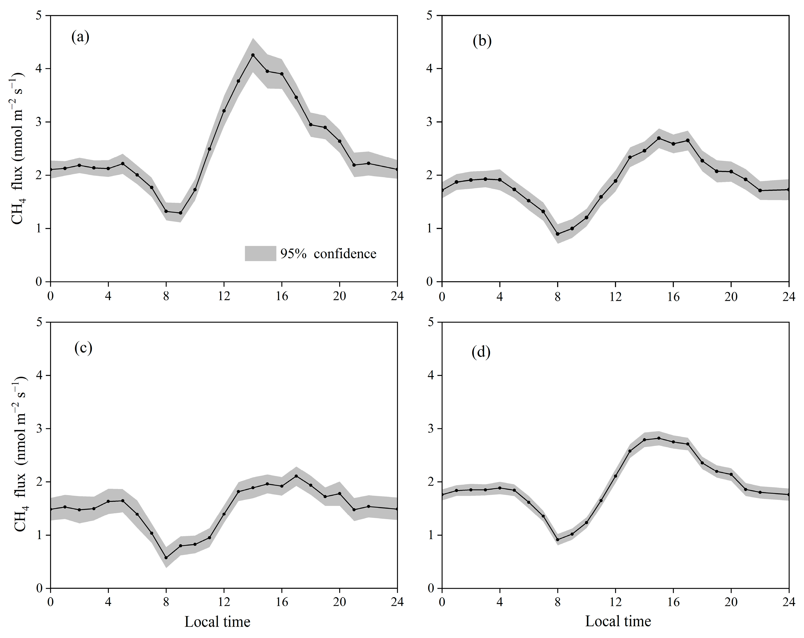
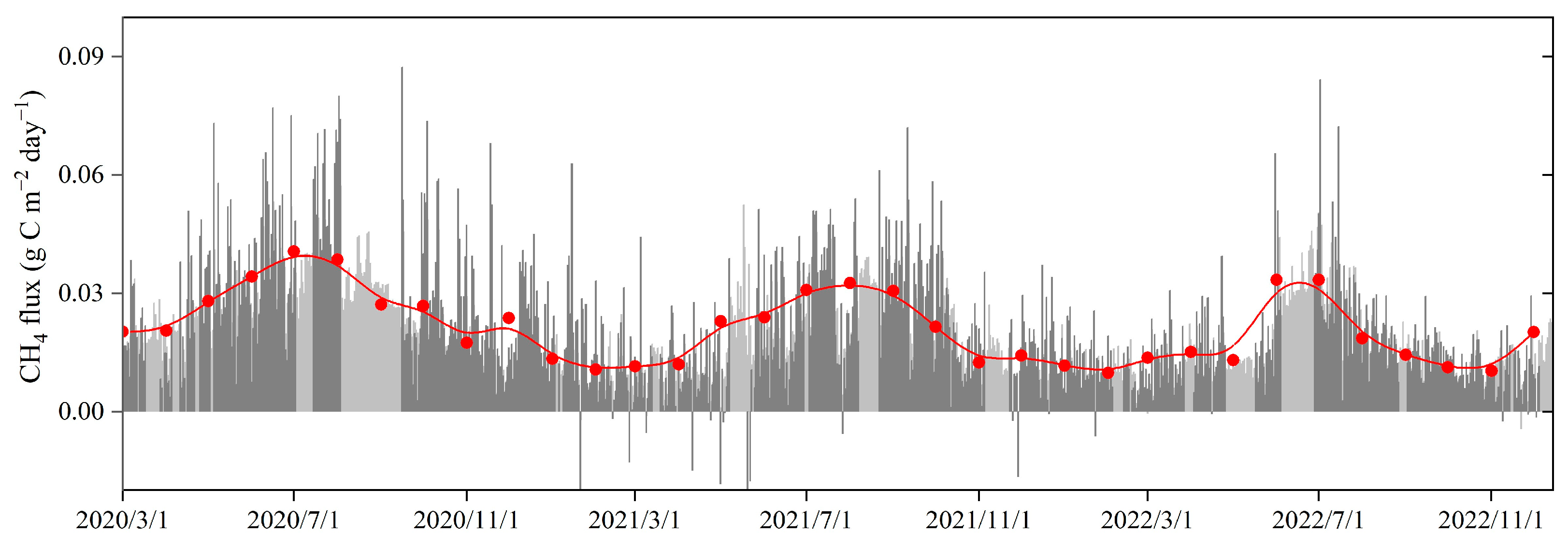
3.2. Temporal Variations in CH4 Fluxes in the Restored Mangrove

The CH4 flux measurements in the restored mangrove fluctuated significantly on the half-hour scale and were mostly positive. The median and mean values of the half-hourly CH4 fluxes were 16.8 and 19.6 nmol m−2 s−1, respectively. Few negative half-hourly CH4 fluxes were observed during the measurement period. When averaged over the entire study duration, the diurnal flux exhibited an M-shaped trend. Specifically, the flux attained a value of 2 nmol m−2 s−1 at midnight, remained stable from midnight until 6 a.m., and subsequently decreased to 0.906 nmol m−2 s−1 by 9 a.m. The second peak in CH4 flux was recorded at 4 p.m. This M-shaped diurnal trend was consistently observed across various years (Figure 3) and has also been documented in wetlands dominated by reeds [49].
The mangrove examined acted consistently as a source of CH4 fluxes throughout the day, with values ranging from −0.256 to 0.288 μmol m−2 s−1. Over the three-year observation period, the daily CH4 flux values were largely above zero, varying from −0.006 to 0.087 g C m−2 day−1, while the monthly averaged daily values ranged between 0.009 and 0.041 g C m−2 day−1 (Figure 4). A clear seasonal trend was observed, with CH4 emissions peaking in the summer and declining during the winter (Figure 4). It is evident that the CH4 emissions from June to September were significantly higher than those in the other months during the study period, cumulatively accounting for as much as 40% of the annual emissions (Figure 4). The overall standard deviation of residual interpolation in the dataset, based on the RF interpolation model, is 0.0281. The CH4 flux showed a decreasing trend over the years, with mean emissions of 9.07, 7.10, and 6.15 g C m−2 year−1 in 2020, 2021, and 2022, respectively.

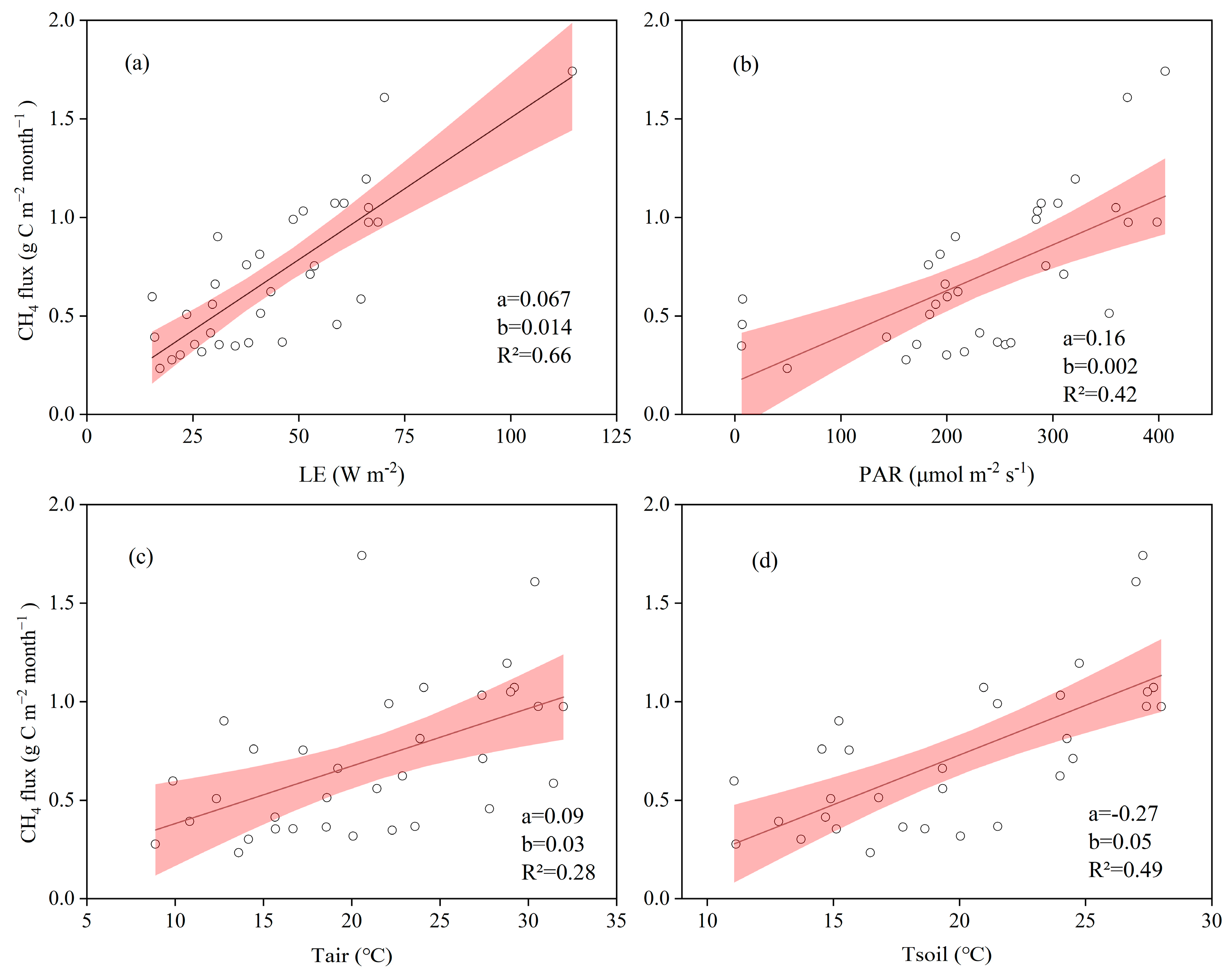
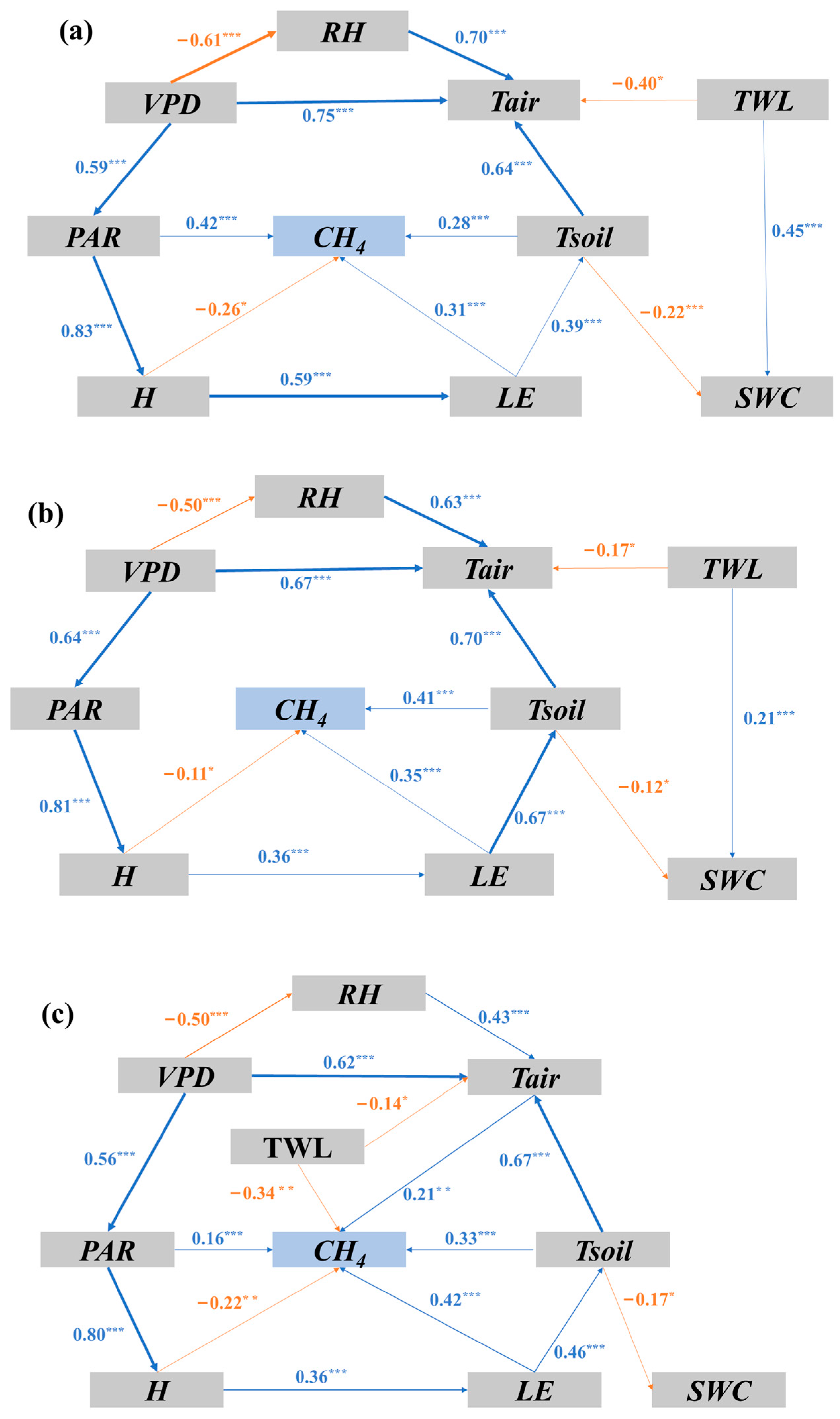
3.3. Biophysical Drivers of CH4 Fluxes in the Restored Mangrove

The heat map revealed significant correlations (p ≤ 0.001) between the daily CH4 flux and several environmental drivers, including LE, H, Tair, Tsoil, PAR, VPD, RH, and TWL (Figure 5). The correlation coefficient (r) for the relationship between LE and CH4 was 0.71 (p ≤ 0.001) in 2022, the highest among all environmental factors during the study period. Different environmental variables were shown to be significantly associated with the CH4 flux during the 3-year period, with Tair (r > 0.6) and Tsoil (r > 0.6) showing the strongest correlations (p ≤ 0.001). The correlations of LE, TWL, and VPD with the CH4 flux increased annually during the study period, while SWC showed a significant correlation only in 2020 (p ≤ 0.001).
The RF model results indicated that LE and rainfall were the dominant factors influencing daily integrated CH4 emissions, as evidenced by feature importance (FI) values of 0.157 and 0.117, respectively (Table 1). Other factors had FI values ranging from 0.031 to 0.086, which were lower than those for them (Table 1). After the screening of stepwise variables, a total of three variables remained, i.e., LE, Tsoil, and rainfall (Table 1). The RF algorithm explained 39% of the variance in daily CH4 emissions, markedly surpassing the stepwise regression model, which accounted for just 18% of the variation. This comparison highlights the superior performance of the RF algorithm compared to conventional statistical methods in tackling ecological issues. Figure 6 presents the linear relationships between the monthly aggregated CH4 emissions and the environmental drivers. On the monthly scale, the integrated CH4 emissions exhibited linear correlations with LE, PAR, Tair, and Tsoil (p < 0.001). The CH4 flux from June to September was significantly higher than in other months, and LE, PAR, Tair, and Tsoil also showed consistent patterns of change.
According to the path analysis findings, the environmental variables were prioritized by their influence on CH4 emissions: Tsoil > LE > PAR > H > TWL (Figure 7). The impact of H and TWL on CH4 emissions was minimal, as their total effect magnitudes were consistently below −0.11 (p ≤ 0.01). On the other hand, Tsoil and LE demonstrated a substantial influence, with their effect magnitudes consistently surpassing 0.28 (p ≤ 0.01). PAR affected CH4 emissions in 2020 and 2022 but not in 2021, while Tair and TWL were shown to influence emissions only in 2022.

4. Discussion

4.1. CH4 Emissions from Natural and Restored Mangrove Ecosystems

The restored mangrove ecosystem, whose location corresponded to the northernmost distribution of mangroves in China, acted as a CH4 source from 2020 to 2022. The daily CH4 flux exhibited a unimodal pattern with values ranging from −0.02 to 0.09 g C m−2 day−1 (Figure 4), showing clear seasonal variation by peaking in summer (June–September) and being lower in winter (December–February). Processes governing CH4 emissions include those related to its production, oxidation, and transport, all of which interact to regulate its levels [33,50]. In this study, the CH4 flux peaked in the late afternoon (between 4 and 6 p.m.; Figure 3), possibly due to a combination of elevated soil temperatures and significantly reduced PAR, which likely led to pronounced CH4 production alongside limited CH4 oxidation [33]. The CH4 flux during the day was often 23% lower than at nighttime (Figure 3), possibly because daytime photosynthesis increased oxygen levels in the mangrove root zones through diffusion via the pneumatophores, which in turn enhanced CH4 oxidation [4,51]. Seasonal fluctuations in CH4 emissions from the restored mangrove, with increased emissions in summer relative to winter, are consistent with patterns observed in other wetlands experiencing similar temperature and precipitation variations [24,52]. Under high temperatures in July and August, plants close their stomata to reduce water transpiration, blocking this important pathway for CH4 emissions and causing them to decrease [53]. The annual CH4 budget of the restored mangrove (7.2 g C m−2 year−1) was below the typical budgets found in inland wetlands (average of 16.5 g C m−2 year−1) [17]. In contrast, it was seven times higher than the median mangrove CH4 budget (1.22 g C m−2 year−1) reported in a global study of 54 mangrove sites [12].
In previous investigations, CH4 emissions from mangrove ecosystems were predominantly quantified using static chambers covering a limited area [54,55,56]. Table 2 shows a comparison between the CH4 flux from our mangrove measured via EC and that from other mangroves measured via EC and chambers in tropical or subtropical regions. In both cases, mangroves were shown to be sources of CH4 emissions, with values ranging from −0.03 to 40.15 g C m−2 year−1. Specifically, chamber measurements covered a range from −0.03 to 11 g C m−2 year−1 and EC measurements from 3.1 to 40.15 g C m−2 year−1 (Table 2).
Due to variations in spatial extent and temporal scales, notable discrepancies have been observed between chamber-based and EC-based studies, indicating that measurements of CH4 flux from the same mangrove forest, when conducted via the EC method, typically yield higher values compared to those obtained using chamber-based approaches [15,57,58].This discrepancy is because the EC technique encompasses all potential CH4 emission pathways within the entire ecosystem [59]. In contrast, the chamber method focuses solely on measuring CH4 fluxes at the boundary between soil and atmosphere within the chamber [15]. The CH4 emissions measured in our restored mangrove fell within these ranges and were slightly lower than those recorded in regions at lower latitudes (Figure 8). CH4 emissions from salt marshes are generally higher than those from mangroves [16,60]. In the salt marshes of the Mississippi River in the United States, which is at a similar latitude to Aojiang station, CH4 emissions (10.35 g C m−2 year−1) are slightly higher than those from Aojiang station [16]. In saline–alkali wetlands at higher latitudes (38.04° N), CH4 emissions can rise up to 58.3 g C m−2 year−1 [60].
Table 2. Comparison of annual CH4 fluxes between restored and natural mangroves across the world.
SiteLocationMethodAnnual CH4 FluxRef
(g C m−2 Year−1)
Sundarbans, IND21.46° S, 81.43° EEddy Covariance40.15[32]
Guangdong, China22.60° N, 113.64° EEddy Covariance25.50[8]
Hong Kang, China22.49° N, 114.02° EEddy Covariance11.70[15]
Zhejiang, China27.58° N, 120.57° EEddy Covariance7.44This study
Pichavaram, IND25.61° S, 79.79° EEddy Covariance6.00[31]
Fujian, China23.92° N, 117.41° EEddy Covariance3.10[33]
Hainan, China19.96° N, 110.58° EChamber11.00[61]
Guangdong, China23.27° N, 116.52° EChamber4.90[62]
Hainan, China19.96°S, 110.54° EChamber3.63[63]
Fujian, China23.92° N, 117.41° EChamber1.83[64]
Hainan, China19.63° N, 110.77° EChamber1.49[55]
Fujian, China23.92° N, 117.41° EChamber1.26[54]
Guangxi, China21.50° N, 109.20° EChamber1.05[65]
Taiwan, China24.68° N, 120.84° EChamber0.88[56]
Fujian, China24.55° N, 118.03° EChamber0.47[66]
Taiwan, China23.36° N, 120.13° EChamber0.15[56]
Guangdong, China22.45° N, 113.63° EChamber-0.03[67]

4.2. Complex Effects of Environmental Factors on CH4 Fluxes in the Restored Mangrove Ecosystem

Although factors such as PAR, Tair, TWL, WS, and LE are recognized as significant environmental influences, their relative impact may differ between various ecosystems [33,42]. Previous studies indicate that the RF algorithm offers benefits compared to conventional statistical approaches, particularly in ecological issues where explanatory variables exhibit high collinearity and nonlinear relationships [15]. Based on the RF model results, LE was found to be the most influential predictor of CH4 emissions in the restored mangrove (Table 1). This parameter exerted an indirect influence on CH4 emissions by augmenting evapotranspiration, thereby facilitating the translocation of CH4 from the soil to the ambient surroundings. In addition, plant rhizome conductance has been shown to assume a pivotal role in controlling emissions across diverse ecosystems [68,69]. Jeffrey et al. [70] found that mangrove tree trunks, particularly those of dead trees, constitute a significant source of CH4 emissions, accounting for 26% of the net ecosystem CH4 flux. Precipitation emerged as the second most significant factor affecting CH4 emissions on the daily scale (Table 1). The significant seasonal fluctuations in precipitation observed in low-latitude regions make this parameter a key regulator of CH4 emissions in wetlands within these areas [15]. In the flooded forests of the Pantanal, CH4 emissions during the dry season were 50 times lower than the average emissions observed during the flood period (0.11 g C m−2 day−1) [52]. As the third most significant environmental factor revealed by the RF model (Table 1), TWL creates an anoxic soil environment that enhances CH4 production by methanogenic bacteria [33,71]. However, due to tidal inundation preventing the gas from being released, the impact on the CH4 flux is delayed.
On the monthly scale, PAR and Tsoil were significantly correlated with CH4 emissions, with R2 values of 0.42 and 0.49, respectively. Peltola et al. [72] and Li et al. [73] both identified soil temperature as a crucial variable for estimating CH4 emissions from EC measurements using RF models. Zhejiang Province represents the northernmost extent of the mangrove habitat in China, and soil temperature in these ecosystems is frequently lower than that in mangroves located at lower latitudes. The monthly average soil temperature does not exceed 30 °C, which is below the optimal range for the activity of methanogenic bacteria (i.e., 33–39 °C; [74]). This explains the significant linear correlation detected between soil temperature and CH4 emissions (p < 0.01). In addition, PAR has been shown to have a pronounced direct influence on the gross primary productivity of mangroves [42], possibly augmenting the channeling effects and thereby leading to increased CH4 fluxes.
Salinity is also a crucial factor influencing CH4 emissions from a biophysical perspective [15,33,75]. Numerous studies have reported an inverse relationship between CH4 emissions and salinity, as sulfate from seawater inhibits CH4 production in tidal wetlands [16,75]. In the Mississippi River salt marsh wetlands, CH4 emissions from brackish areas (46.72 g C m−2 year−1) are much higher than those from freshwater areas (10.35 g C m−2 year−1) [16]. Salt marshes with salinities >18 ppt can have a net radiative cooling effect. Zhu, Qin, and Song [33] also found that in high-salinity areas (>18 ppt), CH4 emissions from mangroves were lower than those from other similar environments. In the Nansha Wetland Park in China, an area with lower salinity (9.41 ppt), the annual emission from mangroves was 24.5 g C m−2 year−1, which was much higher than that recorded in other sites [76]. A previous study of the soils in our restored mangrove showed that soil salinity varied with tidal levels, with values ranging from 10.50 to 13.44 ppt [77]. In future studies, we will measure tidal salinity to examine its correlation with carbon fluxes in mangroves, aiming to deepen our understanding of flux dynamics and their potential impacts.

5. Conclusions

This study examined the CH4 flux from a restored mangrove ecosystem located at the northernmost boundary of China’s mangrove habitat from 2020 to 2022 using the open-path EC system. The annual CH4 emissions recorded in 2020, 2021, and 2022 were 6.15, 7.09, and 9.07 g C m−2 year−1, respectively. The CH4 flux showed strong temporal variations. The seasonal mean CH4 flux in the Aojiang restored mangrove was 170% greater in summer compared to winter, due to elevated temperatures and increased precipitation that enhanced microbial methanogenesis during the warmer months. The combined results of the RF model and path analysis showed that the CH4 emissions from this mangrove ecosystem were mainly influenced by soil temperature and LE. In general, mangroves were revealed as sources of CH4 emissions, which therefore need to be taken into consideration when calculating the carbon balance of these ecosystems. This study highlights the beneficial impacts of mangrove restoration on climate change mitigation and offers valuable insights into the local carbon balance. We also recommend that sustained long-term monitoring is essential for more accurately estimating the carbon budget and its climate impacts.

Author Contributions

Conceptualization, X.L. and P.T.; methodology, L.W.; software, Z.X.; investigation, M.X. and W.C.; resources, H.C.; data curation, Z.Z., M.C. and S.Z.; writing, P.T.; visualization, Y.H.; project administration, X.L. All authors have read and agreed to the published version of the manuscript.

Funding

This work was supported by the National Key Research and Development Program of China (No. 2022YFC3703300) and the BNU-FGS Global Environmental Change Program of Beijing Normal University (No. 2023-GC-ZYTS-07).

Data Availability Statement

Primary data for this research are available at Zenodo via https://doi.org/10.5281/zenodo.11277065, provided by Xu, Li, Tian, Huang, Zhu, Zou, Huang, Zhang, Zhang, and Chen [77].

Acknowledgments

The authors are very grateful to the editors and anonymous reviewers for their valuable time and advice on this manuscript.

Conflicts of Interest

The authors declare no conflicts of interest.

References

  1. Duarte, C.M.; Losada, I.J.; Hendriks, I.E.; Mazarrasa, I.; Marbà, N. The role of coastal plant communities for climate change mitigation and adaptation. Nat. Clim. Chang. 2013, 3, 961–968. [Google Scholar] [CrossRef]
  2. Macreadie, P.I.; Nielsen, D.A.; Kelleway, J.J.; Atwood, T.B.; Seymour, J.R.; Petrou, K.; Connolly, R.M.; Thomson, A.C.G.; Trevathan-Tackett, S.M.; Ralph, P.J. Can we manage coastal ecosystems to sequester more blue carbon? Front. Ecol. Environ. 2017, 15, 206–213. [Google Scholar] [CrossRef]
  3. Nellemann, C.; Corcoran, E.; Duarte, C.M. Blue Carbon: The Role of Healthy Oceans in Binding Carbon—A Rapid Response Assessment. U. N. Environ. Programme GRID 2009, 32, 589–598. [Google Scholar]
  4. Zhu, X.; Sun, C.; Qin, Z. Drought-Induced Salinity Enhancement Weakens Mangrove Greenhouse Gas Cycling. J. Geophys. Res. Biogeosci. 2021, 126, e2021JG006416. [Google Scholar] [CrossRef]
  5. Ouyang, X.; Lee, S. Improved estimates on global carbon stock and carbon pools in tidal wetlands. Nat. Commun. 2020, 11, 317. [Google Scholar] [CrossRef] [PubMed]
  6. Friess, D.A.; Krauss, K.W.; Taillardat, P.; Adame, M.F.; Yando, E.S.; Cameron, C.; Sasmito, S.D.; Sillanpää, M. Mangrove Blue Carbon in the Face of Deforestation, Climate Change, and Restoration. Annu. Plant Rev. 2020, 3, 427–456. [Google Scholar]
  7. Gou, R.; Buchmann, N.; Chi, J.; Luo, Y.; Mo, L.; Shekhar, A.; Feigenwinter, I.; Hörtnagl, L.; Lu, W.; Cui, X. Temporal variations of carbon and water fluxes in a subtropical mangrove forest: Insights from a decade-long eddy covariance measurement. Agric. For. Meteorol. 2023, 343, 109764. [Google Scholar] [CrossRef]
  8. Zhao, X.; Wang, C.; Li, T.; Zhang, C.; Fan, X.; Zhang, Q.; Zhang, Q.; Chen, X.; Zou, X.; Shen, C.; et al. Net CO2 and CH4 emissions from restored mangrove wetland: New insights based on a case study in estuary of the Pearl River, China. Sci. Total Environ. 2022, 811, 151619. [Google Scholar] [CrossRef] [PubMed]
  9. Sasmito, S.D.; Taillardat, P.; Clendenning, J.N.; Cameron, C.; Friess, D.A.; Murdiyarso, D.; Hutley, L.B. Effect of land-use and land-cover change on mangrove blue carbon: A systematic review. Glob. Chang. Biol. 2019, 25, 4291–4302. [Google Scholar] [CrossRef]
  10. Zhu, X.; Chen, J.; Li, L.; Li, M.; Li, T.; Qin, Z.; Wang, F.; Zhao, X. Asynchronous methane and carbon dioxide fluxes drive temporal variability of mangrove blue carbon sequestration. Geophys. Res. Lett. 2024, 51, e2023GL107235. [Google Scholar] [CrossRef]
  11. Macreadie, P.I.; Costa, M.D.; Atwood, T.B.; Friess, D.A.; Kelleway, J.J.; Kennedy, H.; Lovelock, C.E.; Serrano, O.; Duarte, C.M. Blue carbon as a natural climate solution. Nat. Rev. Earth Environ. 2021, 2, 826–839. [Google Scholar] [CrossRef]
  12. Al-Haj, A.N.; Fulweiler, R.W. A synthesis of methane emissions from shallow vegetated coastal ecosystems. Glob. Chang. Biol. 2020, 26, 2988–3005. [Google Scholar] [CrossRef] [PubMed]
  13. Saunois, M.; Stavert, A.R.; Poulter, B.; Bousquet, P.; Canadell, J.G.; Jackson, R.B.; Raymond, P.A.; Dlugokencky, E.J.; Houweling, S.; Patra, P.K. The global methane budget 2000–2017. Earth Syst. Sci. Data Discuss. 2019, 2019, 1561–1623. [Google Scholar] [CrossRef]
  14. Hemes, K.S.; Chamberlain, S.D.; Eichelmann, E.; Knox, S.H.; Baldocchi, D.D. A biogeochemical compromise: The high methane cost of sequestering carbon in restored wetlands. Geophys. Res. Lett. 2018, 45, 6081–6091. [Google Scholar] [CrossRef]
  15. Liu, J.; Zhou, Y.; Valach, A.; Shortt, R.; Kasak, K.; Rey-Sanchez, C.; Hemes, K.S.; Baldocchi, D.; Lai, D.Y.F. Methane emissions reduce the radiative cooling effect of a subtropical estuarine mangrove wetland by half. Glob. Chang. Biol. 2020, 26, 4998–5016. [Google Scholar] [CrossRef] [PubMed]
  16. Holm, G.O.; Perez, B.C.; McWhorter, D.E.; Krauss, K.W.; Johnson, D.J.; Raynie, R.C.; Killebrew, C.J. Ecosystem Level Methane Fluxes from Tidal Freshwater and Brackish Marshes of the Mississippi River Delta: Implications for Coastal Wetland Carbon Projects. Wetlands 2016, 36, 401–413. [Google Scholar] [CrossRef]
  17. Knox, S.H.; Jackson, R.B.; Poulter, B.; McNicol, G.; Fluet-Chouinard, E.; Zhang, Z.; Hugelius, G.; Bousquet, P.; Canadell, J.G.; Saunois, M. FLUXNET-CH4 synthesis activity: Objectives, observations, and future directions. Bull. Am. Meteorol. Soc. 2019, 100, 2607–2632. [Google Scholar] [CrossRef]
  18. Neubauer, S.C.; Megonigal, J.P. Moving beyond global warming potentials to quantify the climatic role of ecosystems. Ecosystems 2015, 18, 1000–1013. [Google Scholar] [CrossRef]
  19. IPCC. Climate Change 2021: Summary for Policymakers; IPCC: Geneva, Switzerland, 2021. [Google Scholar]
  20. Rosentreter, J.A.; Al-Haj, A.N.; Fulweiler, R.W.; Williamson, P. Methane and nitrous oxide emissions complicate coastal blue carbon assessments. Glob. Biogeochem. Cycles 2021, 35, e2020GB006858. [Google Scholar] [CrossRef]
  21. Zheng, Y.; Takeuchi, W. Estimating mangrove forest gross primary production by quantifying environmental stressors in the coastal area. Sci. Rep. 2022, 12, 2238. [Google Scholar] [CrossRef]
  22. Wang, H.; Liao, G.; D’Souza, M.; Yu, X.; Yang, J.; Yang, X.; Zheng, T. Temporal and spatial variations of greenhouse gas fluxes from a tidal mangrove wetland in Southeast China. Environ. Sci. Pollut. Res. 2016, 23, 1873–1885. [Google Scholar] [CrossRef]
  23. Rodda, S.R.; Thumaty, K.C.; Praveen, M.S.S.; Jha, C.S.; Dadhwal, V.K. Multi-year eddy covariance measurements of net ecosystem exchange in tropical dry deciduous forest of India. Agric. For. Meteorol. 2021, 301–302, 108351. [Google Scholar] [CrossRef]
  24. Philipp, K.; Juang, J.-Y.; Deventer, M.J.; Klemm, O. Methane emissions from a subtropical grass marshland, northern Taiwan. Wetlands 2017, 37, 1145–1157. [Google Scholar] [CrossRef]
  25. Nobrega, G.N.; Ferreira, T.O.; Siqueira Neto, M.; Queiroz, H.M.; Artur, A.G.; Mendonca Ede, S.; Silva Ede, O.; Otero, X.L. Edaphic factors controlling summer (rainy season) greenhouse gas emissions (CO2 and CH4) from semiarid mangrove soils (NE-Brazil). Sci. Total Environ. 2016, 542, 685–693. [Google Scholar] [CrossRef] [PubMed]
  26. Meng, Y.; Bai, J.; Gou, R.; Cui, X.; Feng, J.; Dai, Z.; Diao, X.; Zhu, X.; Lin, G. Relationships between above- and below-ground carbon stocks in mangrove forests facilitate better estimation of total mangrove blue carbon. Carbon Balance Manag. 2021, 16, 8. [Google Scholar] [CrossRef]
  27. Kim, Y.; Johnson, M.S.; Knox, S.H.; Black, T.A.; Dalmagro, H.J.; Kang, M.; Kim, J.; Baldocchi, D. Gap-filling approaches for eddy covariance methane fluxes: A comparison of three machine learning algorithms and a traditional method with principal component analysis. Glob. Chang. Biol. 2020, 26, 1499–1518. [Google Scholar] [CrossRef] [PubMed]
  28. Barr, J.G.; Engel, V.; Fuentes, J.D.; Zieman, J.C.; O’Halloran, T.L.; Smith, T.J.; Anderson, G.H. Controls on mangrove forest-atmosphere carbon dioxide exchanges in western Everglades National Park. J. Geophys. Res. Biogeosci. 2010, 115, G02020. [Google Scholar] [CrossRef]
  29. Leopold, A.; Marchand, C.; Renchon, A.; Deborde, J.; Quiniou, T.; Allenbach, M. Net ecosystem CO2 exchange in the “Coeur de Voh” mangrove, New Caledonia: Effects of water stress on mangrove productivity in a semi-arid climate. Agric. For. Meteorol. 2016, 223, 217–232. [Google Scholar] [CrossRef]
  30. Rodda, S.; Thumaty, K.; Jha, C.; Dadhwal, V. Seasonal Variations of Carbon Dioxide, Water Vapor and Energy Fluxes in Tropical Indian Mangroves. Forests 2016, 7, 35. [Google Scholar] [CrossRef]
  31. Gnanamoorthy, P.; Chakraborty, S.; Nagarajan, R.; Ramasubramanian, R.; Selvam, V.; Burman, P.K.D.; Sarathy, P.P.; Zeeshan, M.; Song, Q.; Zhang, Y. Seasonal variation of methane fluxes in a mangrove ecosystem in south India: An eddy covariance-based approach. Estuaries Coasts 2022, 45, 551–566. [Google Scholar] [CrossRef]
  32. Jha, C.S.; Rodda, S.R.; Thumaty, K.C.; Raha, A.; Dadhwal, V. Eddy covariance based methane flux in Sundarbans mangroves, India. J. Earth Syst. Sci. 2014, 123, 1089–1096. [Google Scholar] [CrossRef]
  33. Zhu, X.; Qin, Z.; Song, L. How Land-Sea Interaction of Tidal and Sea Breeze Activity Affect Mangrove Net Ecosystem Exchange? J. Geophys. Res. Atmos. 2021, 126, e2020JD034047. [Google Scholar] [CrossRef]
  34. Zou, H.; Li, X.; Li, S.; Xu, Z.; Yu, Z.; Cai, H.; Chen, W.; Ni, X.; Wu, E.; Zeng, G. Soil organic carbon stocks increased across the tide-induced salinity transect in restored mangrove region. Sci. Rep. 2023, 13, 19758. [Google Scholar] [CrossRef] [PubMed]
  35. Castellví, F.; Perez, P.J.; Villar, J.M.; Rosell, J.I. Analysis of methods for estimating vapor pressure deficits and relative humidity. Agric. For. Meteorol. 1996, 82, 29–45. [Google Scholar] [CrossRef]
  36. Wilczak, J.M.; Oncley, S.P.; Stage, S.A. Sonic anemometer tilt correction algorithms. Bound.-Layer Meteorol. 2001, 99, 127–150. [Google Scholar] [CrossRef]
  37. Fan, S.M.; Wofsy, S.C.; Bakwin, P.S.; Jacob, D.J.; Fitzjarrald, D.R. Atmosphere-Biosphere Exchange of CO2 and O3 in the Central-Amazon-Forest. J. Geophys. Res. Atmos. 1990, 95, 16851–16864. [Google Scholar] [CrossRef]
  38. Moncrieff, J.B.; Massheder, J.M.; de Bruin, H.; Elbers, J.; Friborg, T.; Heusinkveld, B.; Kabat, P.; Scott, S.; Soegaard, H.; Verhoef, A. A system to measure surface fluxes of momentum, sensible heat, water vapour and carbon dioxide. J. Hydrol. 1997, 188, 589–611. [Google Scholar] [CrossRef]
  39. Webb, E.K.; Pearman, G.I.; Leuning, R. Correction of Flux Measurements for Density Effects Due to Heat and Water-Vapor Transfer. Q. J. R. Meteorol. Soc. 1980, 106, 85–100. [Google Scholar] [CrossRef]
  40. Mauder, M.; Foken, T. Documentation and Instruction Manual of the Eddy Covariance Software Package TK2; Universität Bayreuth: Bayreuth, Germany, 2011. [Google Scholar]
  41. Papale, D.; Reichstein, M.; Aubinet, M.; Canfora, E.; Bernhofer, C.; Kutsch, W.; Longdoz, B.; Rambal, S.; Valentini, R.; Vesala, T.; et al. Towards a standardized processing of Net Ecosystem Exchange measured with eddy covariance technique: Algorithms and uncertainty estimation. Biogeosciences 2006, 3, 571–583. [Google Scholar] [CrossRef]
  42. Liu, J.G.; Lai, D.Y.F. Subtropical mangrove wetland is a stronger carbon dioxide sink in the dry than wet seasons. Agric. For. Meteorol. 2019, 278, 107644. [Google Scholar] [CrossRef]
  43. Chen, J. Biophysical Models and Applications in Ecosystem Analysis; Michigan State University Press: East Lansing, MI, USA, 2021. [Google Scholar]
  44. Archer, K.J.; Kimes, R.V. Empirical characterization of random forest variable importance measures. Comput. Stat. Data Anal. 2008, 52, 2249–2260. [Google Scholar] [CrossRef]
  45. Pedregosa, F.; Varoquaux, G.; Gramfort, A.; Michel, V.; Thirion, B.; Grisel, O.; Blondel, M.; Prettenhofer, P.; Weiss, R.; Dubourg, V.; et al. Scikit-learn: Machine Learning in Python. J. Mach. Learn. Res. 2011, 12, 2825–2830. [Google Scholar]
  46. Helman, D.; Osem, Y.; Yakir, D.; Lensky, I.M. Relationships between climate, topography, water use and productivity in two key Mediterranean forest types with different water-use strategies. Agric. For. Meteorol. 2017, 232, 319–330. [Google Scholar] [CrossRef]
  47. Wang, Y.; Zhou, L.; Ping, X.Y.; Jia, Q.Y.; Li, R.P. Ten-year variability and environmental controls of ecosystem water use efficiency in a rainfed maize cropland in Northeast China. Field Crops Res. 2018, 226, 48–55. [Google Scholar] [CrossRef]
  48. Lefcheck, J.S. piecewiseSEM: Piecewise structural equation modelling in r for ecology, evolution, and systematics. Methods Ecol. Evol. 2016, 7, 573–579. [Google Scholar] [CrossRef]
  49. Van Der Nat, F.-F.W.; Middelburg, J.J.; Van Meteren, D.; Wielemakers, A. Diel methane emission patterns from Scirpus lacustris and Phragmites australis. Biogeochemistry 1998, 41, 1–22. [Google Scholar] [CrossRef]
  50. Bridgham, S.D.; Cadillo-Quiroz, H.; Keller, J.K.; Zhuang, Q. Methane emissions from wetlands: Biogeochemical, microbial, and modeling perspectives from local to global scales. Glob. Chang. Biol. 2013, 19, 1325–1346. [Google Scholar] [CrossRef]
  51. Timmers, P.H.; Welte, C.U.; Koehorst, J.J.; Plugge, C.M.; Jetten, M.S.; Stams, A.J. Reverse methanogenesis and respiration in methanotrophic archaea. Archaea 2017, 2017, 1654237. [Google Scholar] [CrossRef] [PubMed]
  52. Dalmagro, H.J.; Zanella de Arruda, P.H.; Vourlitis, G.L.; Lathuilliere, M.J.; de S. Nogueira, J.; Couto, E.G.; Johnson, M.S. Radiative forcing of methane fluxes offsets net carbon dioxide uptake for a tropical flooded forest. Glob. Chang. Biol. 2019, 25, 1967–1981. [Google Scholar] [CrossRef]
  53. Bukoski, J.J.; Dronova, I.; Potts, M.D. Net loss statistics underestimate carbon emissions from mangrove land use and land cover change. Ecography 2022, 2022, e05982. [Google Scholar] [CrossRef]
  54. Gao, C.-H.; Zhang, S.; Ding, Q.-S.; Wei, M.-Y.; Li, H.; Li, J.; Wen, C.; Gao, G.-F.; Liu, Y.; Zhou, J.-J. Source or sink? A study on the methane flux from mangroves stems in Zhangjiang estuary, southeast coast of China. Sci. Total Environ. 2021, 788, 147782. [Google Scholar] [CrossRef]
  55. Zheng, X.; Guo, J.; Song, W.; Feng, J.; Lin, G. Methane emission from mangrove wetland soils is marginal but can be stimulated significantly by anthropogenic activities. Forests 2018, 9, 738. [Google Scholar] [CrossRef]
  56. Lin, C.-W.; Kao, Y.-C.; Chou, M.-C.; Wu, H.-H.; Ho, C.-W.; Lin, H.-J. Methane emissions from subtropical and tropical mangrove ecosystems in Taiwan. Forests 2020, 11, 470. [Google Scholar] [CrossRef]
  57. Krauss, K.W.; Holm, G.O.; Perez, B.C.; McWhorter, D.E.; Cormier, N.; Moss, R.F.; Johnson, D.J.; Neubauer, S.C.; Raynie, R.C. Component greenhouse gas fluxes and radiative balance from two deltaic marshes in Louisiana: Pairing chamber techniques and eddy covariance. J. Geophys. Res. Biogeosci. 2016, 121, 1503–1521. [Google Scholar] [CrossRef]
  58. Petrescu, A.M.R.; Lohila, A.; Tuovinen, J.-P.; Baldocchi, D.D.; Desai, A.R.; Roulet, N.T.; Vesala, T.; Dolman, A.J.; Oechel, W.C.; Marcolla, B. The uncertain climate footprint of wetlands under human pressure. Proc. Natl. Acad. Sci. USA 2015, 112, 4594–4599. [Google Scholar] [CrossRef] [PubMed]
  59. Chen, G.C.; Tam, N.F.Y.; Ye, Y. Summer fluxes of atmospheric greenhouse gases N2O, CH4 and CO2 from mangrove soil in South China. Sci. Total Environ. 2010, 408, 2761–2767. [Google Scholar] [CrossRef] [PubMed]
  60. Chamberlain, S.D.; Hemes, K.S.; Eichelmann, E.; Szutu, D.J.; Verfaillie, J.G.; Baldocchi, D.D. Effect of drought-induced salinization on wetland methane emissions, gross ecosystem productivity, and their interactions. Ecosystems 2020, 23, 675–688. [Google Scholar] [CrossRef]
  61. He, Y.; Guan, W.; Xue, D.; Liu, L.; Peng, C.; Liao, B.; Hu, J.; Yang, Y.; Wang, X.; Zhou, G. Comparison of methane emissions among invasive and native mangrove species in Dongzhaigang, Hainan Island. Sci. Total Environ. 2019, 697, 133945. [Google Scholar] [CrossRef]
  62. Yu, X.; Yang, X.; Wu, Y.; Peng, Y.; Yang, T.; Xiao, F.; Zhong, Q.; Xu, K.; Shu, L.; He, Q. Sonneratia apetala introduction alters methane cycling microbial communities and increases methane emissions in mangrove ecosystems. Soil Biol. Biochem. 2020, 144, 107775. [Google Scholar] [CrossRef]
  63. Sheng, N.; Wu, F.; Liao, B.; Xin, K. Methane and carbon dioxide emissions from cultivated and native mangrove species in Dongzhai Harbor, Hainan. Ecol. Eng. 2021, 168, 106285. [Google Scholar] [CrossRef]
  64. Zhang, C.; Zhang, Y.; Luo, M.; Tan, J.; Chen, X.; Tan, F.; Huang, J. Massive methane emission from tree stems and pneumatophores in a subtropical mangrove wetland. Plant Soil 2022, 473, 489–505. [Google Scholar] [CrossRef]
  65. Liu, J.; Zhan, L.; Ye, W.; Wen, J.; Chen, G.; Li, Y.; Chen, L. Fluxes of dissolved methane and nitrous oxide in the tidal cycle in a mangrove in South China. Environ. Chem. 2021, 18, 261–273. [Google Scholar] [CrossRef]
  66. Chen, J.; Zeng, S.; Gao, M.; Chen, G.; Zhu, H.; Ye, Y. Potential effects of sea level rise on the soil-atmosphere greenhouse gas emissions in Kandelia obovata mangrove forests. Acta Oceanol. Sin. 2023, 42, 25–32. [Google Scholar] [CrossRef]
  67. Xu, Y.; Liao, B.; Jiang, Z.; Xin, K.; Xiong, Y.; Guan, W. Emission of greenhouse gases (CH4 and CO2) into the atmosphere from restored mangrove soil in South China. J. Coast. Res. 2021, 37, 52–58. [Google Scholar] [CrossRef]
  68. Covey, K.R.; Megonigal, J.P. Methane production and emissions in trees and forests. New Phytol. 2019, 222, 35–51. [Google Scholar] [CrossRef] [PubMed]
  69. Morin, T.H. Advances in the eddy covariance approach to CH4 monitoring over two and a half decades. J. Geophys. Res. Biogeosci. 2019, 124, 453–460. [Google Scholar] [CrossRef]
  70. Jeffrey, L.C.; Maher, D.T.; Santos, I.R.; Call, M.; Reading, M.J.; Holloway, C.; Tait, D.R. The spatial and temporal drivers of pCO2, pCH4 and gas transfer velocity within a subtropical estuary. Estuar. Coast. Shelf Sci. 2018, 208, 83–95. [Google Scholar] [CrossRef]
  71. Alongi, D. The contribution of mangrove ecosystems to global carbon cycling and greenhouse gas emissions. In Greenhouse Gas and Carbon Balances in Mangrove Coastal Ecosystems; Maruzen Publishing: Tokyo, Japan, 2007. [Google Scholar]
  72. Peltola, O.; Vesala, T.; Gao, Y.; Räty, O.; Alekseychik, P.; Aurela, M.; Chojnicki, B.; Desai, A.R.; Dolman, A.J.; Euskirchen, E.S. Monthly gridded data product of northern wetland methane emissions based on upscaling eddy covariance observations. Earth Syst. Sci. Data 2019, 11, 1263–1289. [Google Scholar] [CrossRef]
  73. Li, J.; Pei, J.; Fang, C.; Li, B.; Nie, M. Opposing seasonal temperature dependencies of CO2 and CH4 emissions from wetlands. Glob. Chang. Biol. 2022, 29, 1133–1143. [Google Scholar] [CrossRef]
  74. Alongi, D.M. Carbon Cycling and Storage in Mangrove Forests. Annu. Rev. Mar. Sci. 2014, 6, 195–219. [Google Scholar] [CrossRef]
  75. Poffenbarger, H.J.; Needelman, B.A.; Megonigal, J.P. Salinity influence on methane emissions from tidal marshes. Wetlands 2011, 31, 831–842. [Google Scholar] [CrossRef]
  76. Wang, C.; Zhao, X.; Chen, X.; Xiao, C.; Fan, X.; Shen, C.; Sun, M.; Shen, Z.; Zhang, Q. Variations in CO2 and CH4 Exchange in Response to Multiple Biophysical Factors from a Mangrove Wetland Park in Southeastern China. Atmosphere 2023, 14, 805. [Google Scholar] [CrossRef]
  77. Xu, Z.; Li, X.; Tian, P.; Huang, Y.; Zhu, Q.; Zou, H.; Huang, Y.; Zhang, Z.; Zhang, S.; Chen, M. Global warming potentials of CO2 uptake, CH4 emissions, and albedo changes in a restored mangrove ecosystem. J. Geophys. Res. Biogeosci. 2024, 129, e2023JG007924. [Google Scholar] [CrossRef]
Figure 1. Photograph (a) and location (b) of the eddy covariance flux tower established for measuring net ecosystem exchange of greenhouse gases over a restored mangrove in China (c).
Forests 15 01487 g001
Figure 2. Time series plots of measured biophysical variables in the restored mangrove between 2020 and 2022, including (a) daily and monthly average air temperature and daily precipitation, (b) daily and monthly average PAR, (c) daily and monthly average VPD, (d) daily and monthly average LE, and (e) daily average, minimum, and maximum as well as monthly average tidal water levels.
Forests 15 01487 g002
Figure 3. Diurnal patterns of the CH4 flux in 2020 (a), 2021 (b), and 2022 (c), and average pattern for the 3-year period (2020–2022) (d). The gray area denotes the 95% confidence interval.
Forests 15 01487 g003
Figure 4. Daily (gray bars) and monthly (red dots) variations in CH4 flux from March 2020 to December 2020. The lighter gray bars represent daily values filled in using RF model simulations.
Forests 15 01487 g004
Figure 5. Coefficients of correlation between environmental variables and the CH4 flux in (a) 2020, (b) 2021, and (c) 2022. The environmental variables included soil water content (SWC), air temperature (Tair), sensible heat (H), photosynthetically active radiation (PAR), vapor pressure deficit (VPD), soil temperature (Tsoil), rainfall, relative humidity (RH), latent heat (LE), and tide water level (TWL). These parameters are expressed as daily averages, except for precipitation, which, here, is indicated as a cumulative value.
Forests 15 01487 g005
Figure 6. Relationships between the monthly integrated CH4 flux and (a) latent heat, (b) photosynthetically active radiation, (c) air temperature, and (d) soil temperature. All the relationships shown were significant at p ≤ 0.001. Red area represents the 95% confidence interval of the fitted line.
Forests 15 01487 g006
Figure 7. Results of path analysis examining the relationships between the CH4 flux and environmental variables in (a) 2020, (b) 2021, and (c) 2022. The environmental variables included soil water content (SWC), photosynthetically active radiation (PAR), vapor pressure deficit (VPD), sensible heat (H), air temperature (Tair), tide water level (TWL), relative humidity (RH), latent heat (LE), and soil temperature (Tsoil). The values of these parameters are expressed as daily averages. Blue represents a positive effect; orange represents a negative effect. * indicates p < 0.05, ** indicates p < 0.01, and *** indicates p < 0.001.
Forests 15 01487 g007
Figure 8. Latitudinal patterns of CH4 fluxes from mangroves measured using chambers (blue points) and EC (green points), and their regression.
Forests 15 01487 g008
Table 1. Relationships between the CH4 flux and various environmental drivers determined using the RF algorithm and stepwise linear regression.
Environmental DriversStepwise Linear RegressionRandom Forest Algorithm
R2Feature ImportanceSD
LE0.090.1570.012
Tsoil0.180.0440.037
rainfall0.190.1170.017
Tide0.19 a0.0860.014
VPD0.19 a0.0610.018
H0.19 a0.0460.011
PAR0.19 a0.0440.014
SWC0.19 a0.0430.002
TA0.19 a0.0340.020
RH0.19 a0.0310.008
a Variables rejected from the final model.
Disclaimer/Publisher’s Note: The statements, opinions and data contained in all publications are solely those of the individual author(s) and contributor(s) and not of MDPI and/or the editor(s). MDPI and/or the editor(s) disclaim responsibility for any injury to people or property resulting from any ideas, methods, instructions or products referred to in the content.

