
The Characteristics of Visitor Behavior and Driving Factors in Urban Mountain Parks: A Case Study of Fuzhou, China
 , , ,
, , ,
Abstract
:1. Introduction
2. Materials and Methods
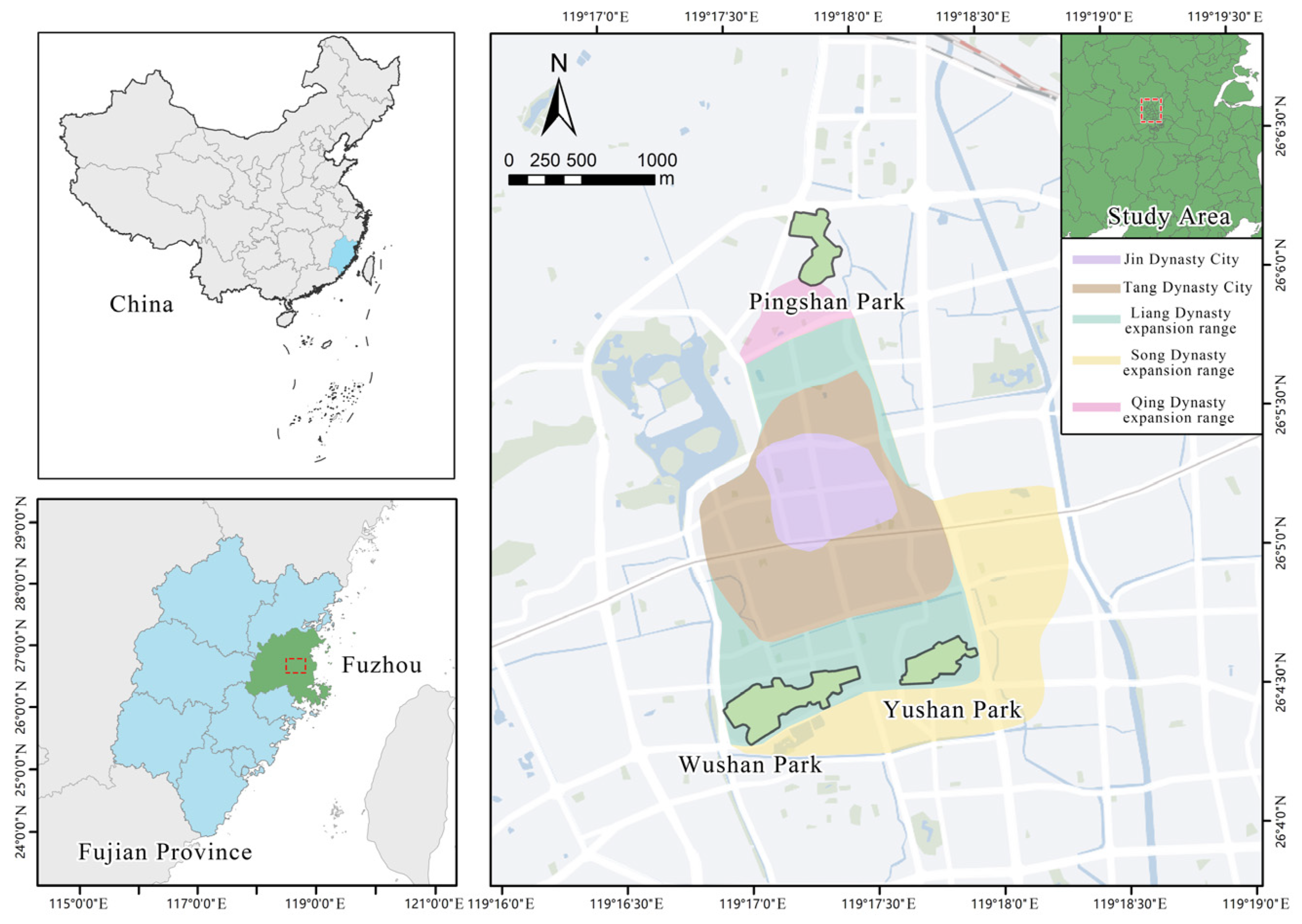
2.1. Research Site
2.2. Spatial Typology
2.3. Data Acquisition
2.3.1. Acquisition of Visitor Behavior Data
2.3.2. Acquisition of Behavioral Driving Factors
2.4. Methodology
2.4.1. Visitor Density Calculator
2.4.2. Tourist Behavioral Diversity Calculator
2.4.3. Tourist Behavioral Variability Calculator
2.4.4. Geographical Detector Model (GDM) Calculation Method
2.5. Data Analysis
3. Results
3.1. Characteristics of Visitors’ Distribution in the Three Mountain Parks
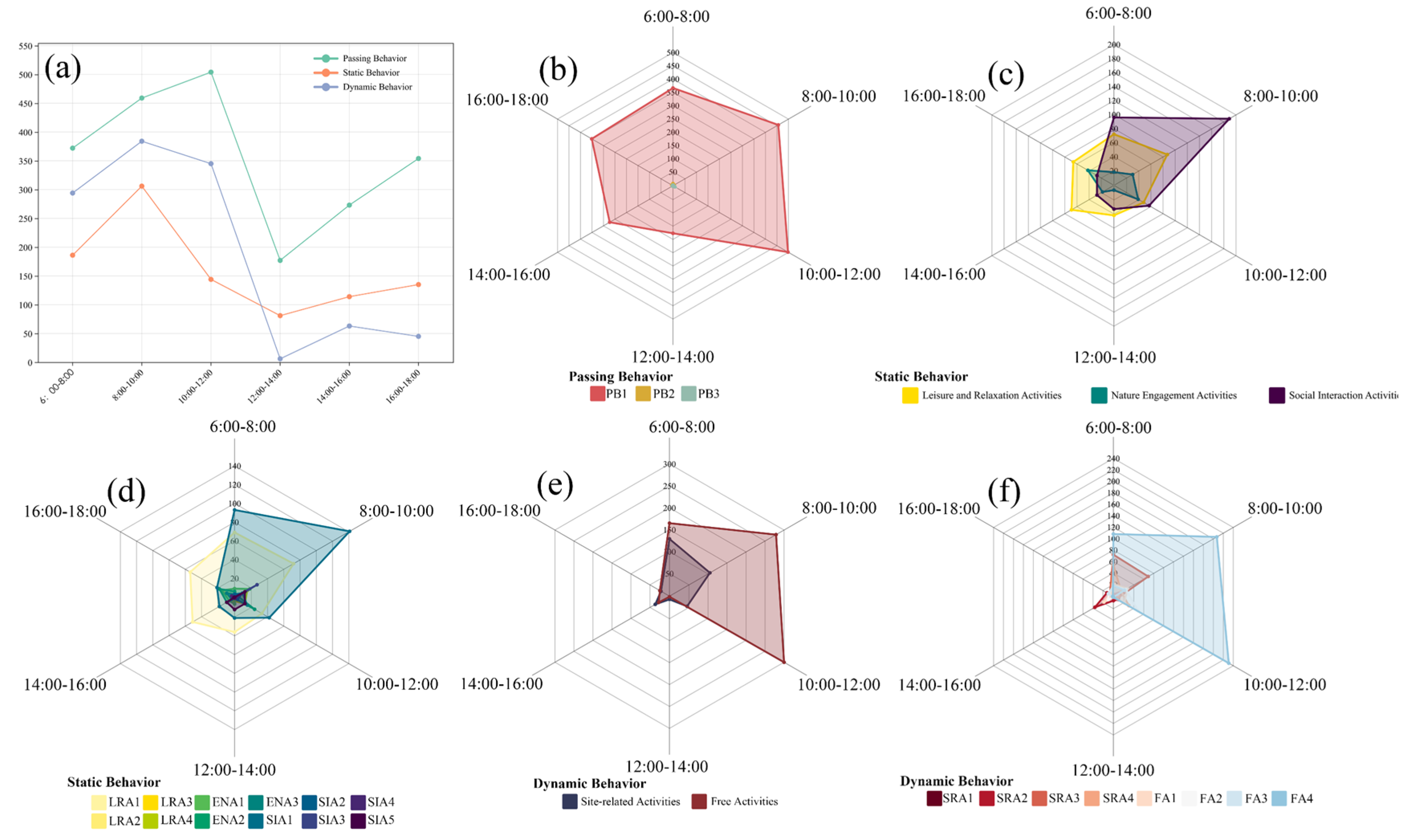
3.1.1. Characteristics of the Overall Number of Visitors’ Behavior
3.1.2. Characteristics of the Spatial and Temporal Distribution of Visitors’ Behavior
3.2. Characteristics of Behavioral Diversity
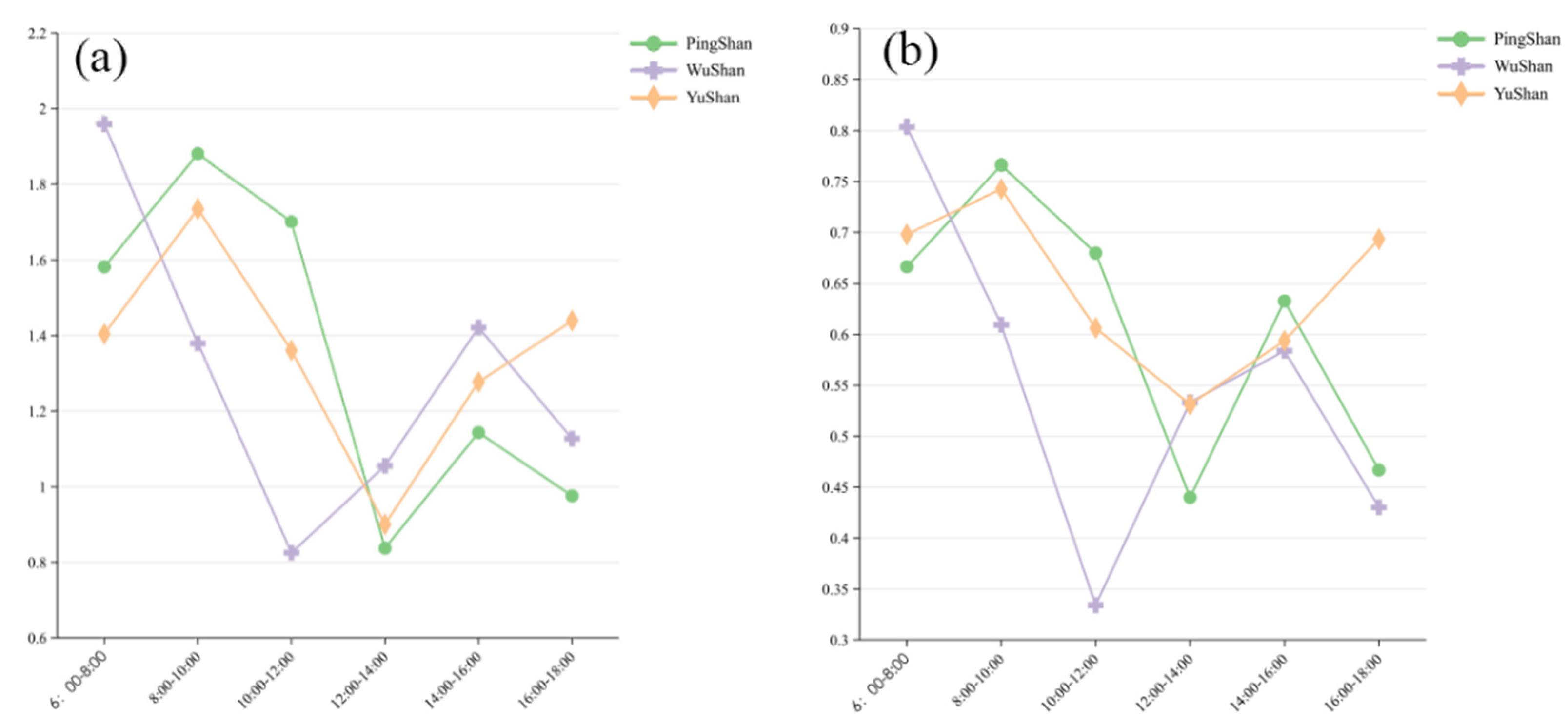
3.2.1. Distribution of Behavioral Diversity
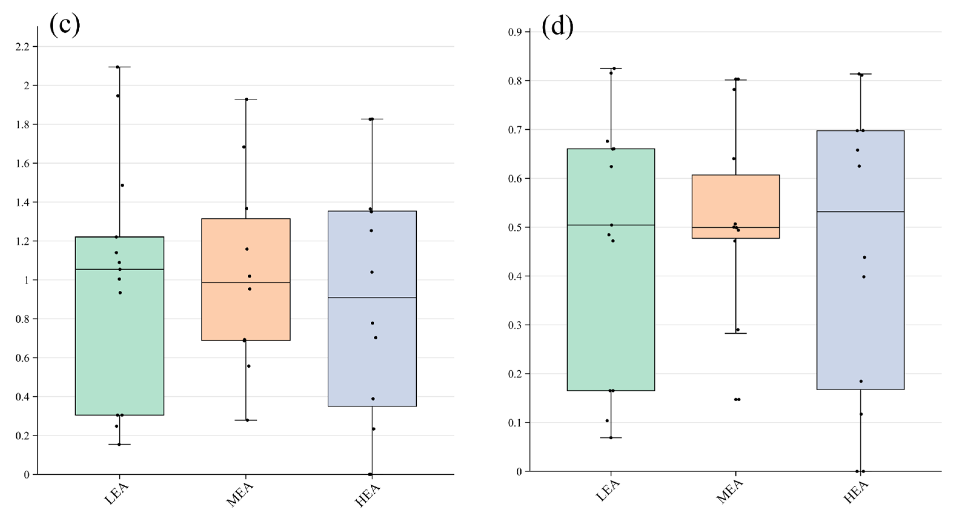
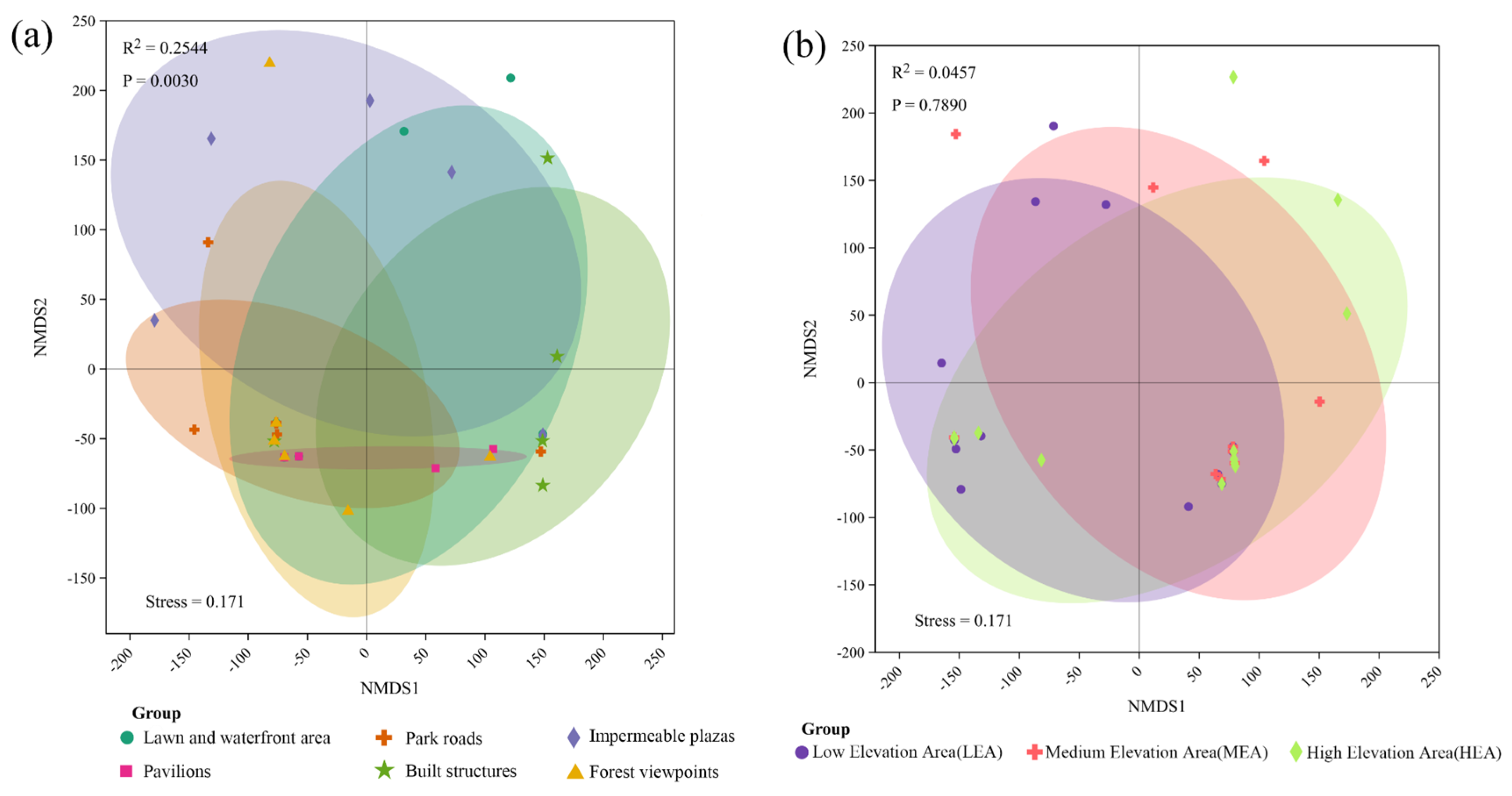
3.2.2. Differences in Behavioral Composition between Spaces
3.3. Visitor Behavior Relevance Exploration
3.3.1. Environmental Factors That Influence Recreational Behavior
3.3.2. Landscape Pattern Factors That Influence Recreational Behavior
3.3.3. Extraction of Major Landscape Factors
3.4. Driving Factor Analysis
3.4.1. Analysis of Visitors’ Behavior Drivers
3.4.2. Analysis of Behavioral Diversity Driver
4. Discussion
4.1. Characteristics of Visitors’ Recreational Behavior
4.2. Environmental Factors That Influence the Behavior of Tourists
4.3. Limitations and Perspectives
5. Conclusions
Author Contributions
Funding
Data Availability Statement
Acknowledgments
Conflicts of Interest
References
- Yeh, C.; Huang, S. Global urbanization and demand for natural resources. In Carbon Sequestration in Urban Ecosystems; Springer: Berlin/Heidelberg, Germany, 2012; pp. 355–371. [Google Scholar]
- Gianfredi, V.; Buffoli, M.; Rebecchi, A.; Croci, R.; Oradini-Alacreu, A.; Stirparo, G.; Marino, A.; Odone, A.; Capolongo, S.; Signorelli, C. Urban Green Spaces and Public Health Outcomes: A systematic review of literature. Eur. J. Public Health 2021, 31, b164–b638. [Google Scholar] [CrossRef]
- Buxbaum, O.; Buxbaum, O. The SOR-model. In Key Insights into Basic Mechanisms of Mental Activity; Springer: Berlin/Heidelberg, Germany, 2016; pp. 7–9. [Google Scholar]
- Jie, D. The Influence of Functional Attributes of Forest Wellness Tourism Destination on Tourists’ Behavioral Intention Based on SOR Theory. Tour. Manag. Technol. Econ. 2023, 6, 53–62. [Google Scholar]
- Jiang, J. The role of natural soundscape in nature-based tourism experience: An extension of the stimulus–organism–response model. Curr. Issues Tour. 2022, 25, 707–726. [Google Scholar] [CrossRef]
- Jabbar, M.; Yusoff, M.M.; Shafie, A. Assessing the role of urban green spaces for human well-being: A systematic review. Geojournal 2022, 87, 4405–4423. [Google Scholar] [CrossRef] [PubMed]
- Larson, L.R.; Jennings, V.; Cloutier, S.A. Public parks and wellbeing in urban areas of the United States. PLoS ONE 2016, 11, e153211. [Google Scholar] [CrossRef] [PubMed]
- Ullah, H.; Wan, W.; Ali Haidery, S.; Khan, N.U.; Ebrahimpour, Z.; Luo, T. Analyzing the spatiotemporal patterns in green spaces for urban studies using location-based social media data. ISPRS Int. J. Geo-Inf. 2019, 8, 506. [Google Scholar] [CrossRef]
- Liu, J.; Kang, J.; Behm, H.; Luo, T. Effects of landscape on soundscape perception: Soundwalks in city parks. Landscape Urban Plan. 2014, 123, 30–40. [Google Scholar] [CrossRef]
- Matsinos, Y.G.; Mazaris, A.D.; Papadimitriou, K.D.; Mniestris, A.; Hatzigiannidis, G.; Maioglou, D.; Pantis, J.D. Spatio-temporal variability in human and natural sounds in a rural landscape. Landscape Ecol. 2008, 23, 945–959. [Google Scholar] [CrossRef]
- Daniel, T.C. Whither scenic beauty? Visual landscape quality assessment in the 21st century. Landscape Urban Plan. 2001, 54, 267–281. [Google Scholar] [CrossRef]
- Dramstad, W.E.; Tveit, M.S.; Fjellstad, W.J.; Fry, G.L. Relationships between visual landscape preferences and map-based indicators of landscape structure. Landscape Urban Plan. 2006, 78, 465–474. [Google Scholar] [CrossRef]
- Quintal, V.A.; Lwin, M.; Phau, I.; Lee, S. Personality attributes of botanic parks and their effects on visitor attitude and behavioural intentions. J. Vacat. Mark. 2019, 25, 176–192. [Google Scholar] [CrossRef]
- Wang, D.; Brown, G.; Liu, Y.; Mateo-Babiano, I. A comparison of perceived and geographic access to predict urban park use. Cities 2015, 42, 85–96. [Google Scholar] [CrossRef]
- Wang, M.; Liu, S.; Wang, C. Spatial distribution and influencing factors of high-quality tourist attractions in Shandong Province, China. PLoS ONE 2023, 18, e288472. [Google Scholar] [CrossRef]
- Li, F.; Li, F.; Li, S.; Long, Y. Deciphering the recreational use of urban parks: Experiments using multi-source big data for all Chinese cities. Sci. Total Environ. 2020, 701, 134896. [Google Scholar] [CrossRef]
- Jian, Z.; Hao, S. Geo-spatial analysis and optimization strategy of park green space landscape pattern of Garden City—A case study of the central district of Mianyang City Sichuan Province. Eur. J. Remote Sens. 2020, 53, 309–315. [Google Scholar] [CrossRef]
- Wartmann, F.M.; Frick, J.; Kienast, F.; Hunziker, M. Factors influencing visual landscape quality perceived by the public. Results from a national survey. Landscape Urban Plan. 2021, 208, 104024. [Google Scholar] [CrossRef]
- Svobodova, K.; Vondrus, J.; Filova, L.; Besta, M. The role of familiarity with the landscape in visual landscape preferences. J. Landsc. Stud. 2011, 4, 11–24. [Google Scholar]
- Skřivanová, Z.; Kalivoda, O.; Sklenička, P. Driving factors for visual landscape preferences in protected landscape areas. Sci. Agric. Bohem. 2014, 45, 36–43. [Google Scholar] [CrossRef]
- Zhou, X.; Cen, Q.; Qiu, H. Effects of urban waterfront park landscape elements on visual behavior and public preference: Evidence from eye-tracking experiments. Urban For. Urban Green. 2023, 82, 127889. [Google Scholar] [CrossRef]
- Zhai, Y.; Baran, P. Application of space syntax theory in study of urban parks and walking. In Proceedings of the Ninth International Space Syntax Symposium, Seoul, Republic of Korea, 31 October–3 November 2013; Sejong University Press: Seoul, Republic of Korea, 2013; pp. 1–13. [Google Scholar]
- Gustafson, E.J. Quantifying landscape spatial pattern: What is the state of the art? Ecosystems 1998, 1, 143–156. [Google Scholar] [CrossRef]
- Wang, J.; Zhang, T.; Fu, B. A measure of spatial stratified heterogeneity. Ecol. Indic. 2016, 67, 250–256. [Google Scholar] [CrossRef]
- Luo, L.; Mei, K.; Qu, L.; Zhang, C.; Chen, H.; Wang, S.; Di, D.; Huang, H.; Wang, Z.; Xia, F. Assessment of the Geographical Detector Method for investigating heavy metal source apportionment in an urban watershed of Eastern China. Sci. Total Environ. 2019, 653, 714–722. [Google Scholar] [CrossRef] [PubMed]
- García-Ayllón, S.; Martínez, G. Analysis of correlation between anthropization phenomena and landscape values of the territory: A GIS framework based on spatial statistics. ISPRS Int. J. Geo-Inf. 2023, 12, 323. [Google Scholar] [CrossRef]
- Wang, S.; Wang, M.; Liu, Y. Access to urban parks: Comparing spatial accessibility measures using three GIS-based approaches. Comput. Environ. Urban Syst. 2021, 90, 101713. [Google Scholar] [CrossRef]
- Heikinheimo, V.; Tenkanen, H.; Bergroth, C.; Järv, O.; Hiippala, T.; Toivonen, T. Understanding the use of urban green spaces from user-generated geographic information. Landscape Urban Plan. 2020, 201, 103845. [Google Scholar] [CrossRef]
- Huang, Z.; Dong, J.; Chen, Z.; Zhao, Y.; Huang, S.; Xu, W.; Zheng, D.; Huang, P.; Fu, W. Spatiotemporal characteristics of public recreational activity in urban green space under summer heat. Forests 2022, 13, 1268. [Google Scholar] [CrossRef]
- Chen, J.; van den Bosch, C.C.K.; Lin, C.; Liu, F.; Huang, Y.; Huang, Q.; Wang, M.; Zhou, Q.; Dong, J. Effects of personality, health and mood on satisfaction and quality perception of urban mountain parks. Urban For. Urban Green. 2021, 63, 127210. [Google Scholar]
- Chen, Z.; Sheng, Y.; Luo, D.; Huang, Y.; Huang, J.; Zhu, Z.; Yao, X.; Fu, W.; Dong, J.; Lan, Y. Landscape Characteristics in Mountain Parks across Different Urban Gradients and Their Relationship with Public Response. Forests 2023, 14, 2406. [Google Scholar] [CrossRef]
- Creany, N.; Monz, C.A.; Esser, S.M. Understanding visitor attitudes towards the timed-entry reservation system in Rocky Mountain National Park: Contemporary managed access as a social-ecological system. J. Outdoor Recreat. Tour. 2024, 45, 100736. [Google Scholar] [CrossRef]
- Huang, X.; Li, M.; Zhang, J.; Zhang, L.; Zhang, H.; Yan, S. Tourists’ spatial-temporal behavior patterns in theme parks: A case study of Ocean Park Hong Kong. J. Destin. Mark. Manag. 2020, 15, 100411. [Google Scholar] [CrossRef]
- Zheng, Y.; Mou, N.; Zhang, L.; Makkonen, T.; Yang, T. Chinese tourists in Nordic countries: An analysis of spatio-temporal behavior using geo-located travel blog data. Comput. Environ. Urban Syst. 2021, 85, 101561. [Google Scholar] [CrossRef] [PubMed]
- Yao, Q.; Shi, Y.; Li, H.; Wen, J.; Xi, J.; Wang, Q. Understanding the tourists’ Spatio-Temporal behavior using open GPS trajectory data: A case study of yuanmingyuan park (Beijing, China). Sustainability 2020, 13, 94. [Google Scholar] [CrossRef]
- Liu, Y.; Lu, A.; Yang, W.; Tian, Z. Investigating factors influencing park visit flows and duration using mobile phone signaling data. Urban For. Urban Green. 2023, 85, 127952. [Google Scholar] [CrossRef]
- Wang, X.; Wu, C. An observational study of park attributes and physical activity in neighborhood parks of Shanghai, China. Int. J. Environ. Res. Public Health 2020, 17, 2080. [Google Scholar] [CrossRef] [PubMed]
- Park, K. Park and neighborhood attributes associated with park use: An observational study using unmanned aerial vehicles. Environ. Behav. 2020, 52, 518–543. [Google Scholar] [CrossRef]
- Xia, J.C.; Zeephongsekul, P.; Packer, D. Spatial and temporal modelling of tourist movements using Semi-Markov processes. Tour. Manag. 2011, 32, 844–851. [Google Scholar] [CrossRef]
- Shoval, N.; Isaacson, M. Tracking tourists in the digital age. Ann. Tour. Res. 2007, 34, 141–159. [Google Scholar] [CrossRef]
- Cheng, B.; Gou, Z.; Zhang, F.; Feng, Q.; Huang, Z. Thermal comfort in urban mountain parks in the hot summer and cold winter climate. Sustain. Cities Soc. 2019, 51, 101756. [Google Scholar] [CrossRef]
- Wang, H.; Qin, F.; Xu, C.; Li, B.; Guo, L.; Wang, Z. Evaluating the suitability of urban development land with a Geodetector. Ecol. Indic. 2021, 123, 107339. [Google Scholar] [CrossRef]
- Liang, Y.; Xu, C. Knowledge diffusion of Geodetector: A perspective of the literature review and Geotree. Heliyon 2023, 9, E19651. [Google Scholar] [CrossRef]
- Qi, J.; Mazumdar, S.; Vasconcelos, A.C. Understanding the Relationship between Urban Public Space and Social Cohesion: A Systematic Review. Int. J. Community Well-Being 2024, 7, 1–58. [Google Scholar] [CrossRef]
- Evenson, K.R.; Jones, S.A.; Holliday, K.M.; Cohen, D.A.; McKenzie, T.L. Park characteristics, use, and physical activity: A review of studies using SOPARC (System for Observing Play and Recreation in Communities). Prev. Med. 2016, 86, 153–166. [Google Scholar] [CrossRef] [PubMed]
- Kordi, A.O.; Galal Ahmed, K. Towards a socially vibrant city: Exploring urban typologies and morphologies of the emerging “CityWalks” in Dubai. City Territ. Archit. 2023, 10, 34. [Google Scholar] [CrossRef]
- Cabanek, A.; Zingoni De Baro, M.E.; Newman, P. Biophilic streets: A design framework for creating multiple urban benefits. Sustain. Earth 2020, 3, 7. [Google Scholar] [CrossRef]
- Liu, H.; Huang, B.; Cheng, X.; Yin, M.; Shang, C.; Luo, Y.; He, B. Sensing-based park cooling performance observation and assessment: A review. Build Environ. 2023, 245, 110915. [Google Scholar] [CrossRef]
- Li, J.; Huang, Z.; Zheng, D.; Zhao, Y.; Huang, P.; Huang, S.; Fang, W.; Fu, W.; Zhu, Z. Effect of landscape elements on public psychology in urban park waterfront green space: A quantitative study by semantic segmentation. Forests 2023, 14, 244. [Google Scholar] [CrossRef]
- Xu, Y.; Chen, X. Uncovering the relationship among spatial vitality, perception, and environment of urban underground space in the metro zone. Undergr. Space 2023, 12, 167–182. [Google Scholar]
- Can Traunmüller, I.; İnce Keller, İ.; Şenol, F. Application of space syntax in neighbourhood park research: An investigation of multiple socio-spatial attributes of park use. Local Environ. 2023, 28, 529–546. [Google Scholar]
- Li, B.; Shi, X.; Wang, H.; Qin, M. Analysis of the relationship between urban landscape patterns and thermal environment: A case study of Zhengzhou City, China. Environ. Monit. Assess. 2020, 192, 540. [Google Scholar]
- Mao, Q.; Sun, J.; Deng, Y.; Wu, Z.; Bai, H. Assessing effects of multi-scale landscape pattern and habitats attributes on taxonomic and functional diversity of Urban River birds. Diversity 2023, 15, 486. [Google Scholar] [CrossRef]
- Ostermann, F.O. Digital representation of park use and visual analysis of visitor activities. Comput. Environ. Urban Syst. 2010, 34, 452–464. [Google Scholar] [CrossRef]
- Sueur, J.; Pavoine, S.; Hamerlynck, O.; Duvail, S. Rapid acoustic survey for biodiversity appraisal. PLoS ONE 2008, 3, e4065. [Google Scholar] [CrossRef] [PubMed]
- Shannon, C.E. A mathematical theory of communication. Bell Syst. Tech. J. 1948, 27, 379–423. [Google Scholar] [CrossRef]
- Simpson, E.H. Measurement of diversity. Nature 1949, 163, 688. [Google Scholar] [CrossRef]
- Bray, J.R.; Curtis, J.T. An ordination of the upland forest communities of southern Wisconsin. Ecol. Monogr. 1957, 27, 326–349. [Google Scholar] [CrossRef]
- Zhu, L.; Meng, J.; Zhu, L. Applying Geodetector to disentangle the contributions of natural and anthropogenic factors to NDVI variations in the middle reaches of the Heihe River Basin. Ecol. Indic. 2020, 117, 106545. [Google Scholar] [CrossRef]
- Duo, L.; Wang, J.; Zhang, F.; Xia, Y.; Xiao, S.; He, B.-J. Assessing the Spatiotemporal Evolution and Drivers of Ecological Environment Quality Using an Enhanced Remote Sensing Ecological Index in Lanzhou City, China. Remote Sens. 2023, 15, 4704. [Google Scholar] [CrossRef]
- Wang, J.F.; Li, X.H.; Christakos, G.; Liao, Y.L.; Zhang, T.; Gu, X.; Zheng, X.Y. Geographical detectors-based health risk assessment and its application in the neural tube defects study of the Heshun Region, China. Int. J. Geogr. Inf. Sci. 2010, 24, 107–127. [Google Scholar] [CrossRef]
- Chacón-Borrego, F.; Corral-Pernía, J.A.; Martínez-Martínez, A.; Castañeda-Vázquez, C. Usage behaviour of public spaces associated with sport and recreational activities. Sustainability 2018, 10, 2377. [Google Scholar] [CrossRef]
- Del Deporte Andaluz, O. Hábitos y Actitudes de la Población Andaluza Ante el Deporte. 2012. Encuentro Nacional de Observatorios del Deporte. Consejería de Turismo, Comercio y Deporte. Junta de Andalucía 2012. Available online: https://www.munideporte.com/seccion/Actualidad/15485/Andalucia:-Habitos-y-Actitudes-de-la-poblacion-ante-el-deporte-2012.html (accessed on 3 March 2024).
- Marques, J.; Teixeira, M. The Elderly and Leisure Activities: A Case Study. Eur. J. Interdiscip. Stud. 2022, 8, 49–67. [Google Scholar] [CrossRef]
- Qi, J.; Ding, L.; Lim, S. A decision-making framework to support urban heat mitigation by local governments. Resour. Conserv. Recycl. 2022, 184, 106420. [Google Scholar] [CrossRef]
- Onose, D.A.; Iojă, I.C.; Niță, M.R.; Vânău, G.O.; Popa, A.M. Too old for recreation? How friendly are urban parks for elderly people? Sustainability 2020, 12, 790. [Google Scholar] [CrossRef]
- Qi, J.; Ding, L.; Lim, S. Application of a decision-making framework for multi-objective optimisation of urban heat mitigation strategies. Urban Clim. 2023, 47, 101372. [Google Scholar] [CrossRef]
- Wang, X.; Li, G.; Pan, J.; Shen, J.; Han, C. The difference in the elderly’s visual impact assessment of pocket park landscape. Sci. Rep. 2023, 13, 16895. [Google Scholar] [CrossRef]
- Zhu, W.; Chi, A.; Sun, Y. Physical activity among older Chinese adults living in urban and rural areas: A review. J. Sport Health Sci. 2016, 5, 281–286. [Google Scholar] [CrossRef]
- Sadia, T. Exploring the Design Preferences of Neurodivergent Populations for Quiet Spaces. 2020. Available online: https://www.researchgate.net/publication/347809450_Exploring_the_Design_Preferences_of_Neurodivergent_Populations_for_Quiet_Spaces (accessed on 3 March 2024).
- Xiang, Y.; Meng, Q.; Zhang, X.; Li, M.; Yang, D.; Wu, Y. Soundscape diversity: Evaluation indices of the sound environment in urban green spaces–Effectiveness, role, and interpretation. Ecol. Indic. 2023, 154, 110725. [Google Scholar] [CrossRef]
- Wang, X.; Tang, P.; He, Y.; Woolley, H.; Hu, X.; Yang, L.; Luo, J. The correlation between children’s outdoor activities and community space characteristics: A case study utilizing SOPARC and KDE methods in Chengdu, China. Cities 2024, 150, 105002. [Google Scholar] [CrossRef]
- Park, K.; Ewing, R. The usability of unmanned aerial vehicles (UAVs) for measuring park-based physical activity. Landscape Urban Plan. 2017, 167, 157–164. [Google Scholar] [CrossRef]
- Beals, E.W. Bray-Curtis ordination: An effective strategy for analysis of multivariate ecological data. In Advances in Ecological Research; Elsevier: Amsterdam, The Netherlands, 1984; Volume 14, pp. 1–55. [Google Scholar]
- Ricotta, C.; Podani, J. On some properties of the Bray-Curtis dissimilarity and their ecological meaning. Ecol. Complex. 2017, 31, 201–205. [Google Scholar] [CrossRef]
- Kou, R.; Hunter, R.F.; Cleland, C.; Ellis, G. Physical environmental factors influencing older adults’ park use: A qualitative study. Urban For. Urban Green. 2021, 65, 127353. [Google Scholar] [CrossRef]
- Apollo, M.; Andreychouk, V.; Moolio, P.; Wengel, Y.; Myga-Piątek, U. Does the altitude of habitat influence residents’ attitudes to guests? A new dimension in the residents’ attitudes to tourism. J. Outdoor Recreat. Tour. 2020, 31, 100312. [Google Scholar] [CrossRef]
- Zhang, S.; Li, X.; Yang, M.; Song, H. Older adults’ heterogeneous preferences for climate-proof urban blue-green spaces: A case of Chengdu, China. Urban For. Urban Green. 2023, 90, 128139. [Google Scholar] [CrossRef]
- GB 51192-2016; Code for the Design of Public Park. China. 2016. Available online: https://www.mystandards.biz/standard/gb-51192-2016-26.8.2016.html (accessed on 3 March 2024).
- Yun, H.; Kang, D.; Kang, Y. Outdoor recreation planning and management considering FROS and Carrying capacities: A case study of forest wetland in Yeongam-gum, South Korea. Environ. Dev. Sustain. 2022, 24, 502–526. [Google Scholar] [CrossRef]
- Lee, J.; Hwang, H.; Eum, T.; Bae, H.; Rhim, S. Cascade effects of slope gradient on ground vegetation and small-rodent populations in a forest ecosystem. Anim. Biol. 2020, 70, 203–213. [Google Scholar] [CrossRef]
- Arifwidodo, S.D.; Chandrasiri, O. Association between park characteristics and park-based physical activity using systematic observation: Insights from Bangkok, Thailand. Sustainability 2020, 12, 2559. [Google Scholar] [CrossRef]
- Roemmich, J.N.; Epstein, L.H.; Raja, S.; Yin, L.; Robinson, J.; Winiewicz, D. Association of access to parks and recreational facilities with the physical activity of young children. Prev. Med. 2006, 43, 437–441. [Google Scholar] [CrossRef]
- Werneck, A.O.; Oyeyemi, A.L.; Araújo, R.H.; Barboza, L.L.; Szwarcwald, C.L.; Silva, D.R. Association of public physical activity facilities and participation in community programs with leisure-time physical activity: Does the association differ according to educational level and income? BMC Public Health 2022, 22, 279. [Google Scholar] [CrossRef]
- Cerin, E.; Lee, K.; Barnett, A.; Sit, C.H.; Cheung, M.; Chan, W. Objectively-measured neighborhood environments and leisure-time physical activity in Chinese urban elders. Prev. Med. 2013, 56, 86–89. [Google Scholar] [CrossRef]
- Henderson, K.A. Urban parks and trails and physical activity. Ann. Leis. Res. 2006, 9, 201–213. [Google Scholar] [CrossRef]
- McCormack, G.R.; Rock, M.; Toohey, A.M.; Hignell, D. Characteristics of urban parks associated with park use and physical activity: A review of qualitative research. Health Place 2010, 16, 712–726. [Google Scholar] [CrossRef]
- Zhang, R.; Wulff, H.; Duan, Y.; Wagner, P. Associations between the physical environment and park-based physical activity: A systematic review. J. Sport Health Sci. 2019, 8, 412–421. [Google Scholar] [CrossRef] [PubMed]
- Ries, A.V.; Voorhees, C.C.; Roche, K.M.; Gittelsohn, J.; Yan, A.F.; Astone, N.M. A quantitative examination of park characteristics related to park use and physical activity among urban youth. J. Adolescent Health 2009, 45, S64–S70. [Google Scholar] [CrossRef] [PubMed]
- Heinrich, K.M.; Haddock, C.K.; Jitnarin, N.; Hughey, J.; Berkel, L.A.; Poston, W.S. Perceptions of important characteristics of physical activity facilities: Implications for engagement in walking, moderate and vigorous physical activity. Front. Public Health 2017, 5, 319. [Google Scholar] [CrossRef] [PubMed]
- Humpel, N.; Owen, N.; Leslie, E. Environmental factors associated with adults’ participation in physical activity: A review. Am. J. Prev. Med. 2002, 22, 188–199. [Google Scholar] [CrossRef] [PubMed]
- Stewart, O.T.; Moudon, A.V.; Littman, A.; Seto, E.; Saelens, B.E. The association between park facilities and the occurrence of physical activity during park visits. J. Leisure Res. 2018, 49, 217–235. [Google Scholar] [CrossRef]
- Lee, K.Y.; Lee, P.H.; Macfarlane, D. Associations between moderate-to-vigorous physical activity and neighbourhood recreational facilities: The features of the facilities matter. Int. J. Environ. Res. Public Health 2014, 11, 12594–12610. [Google Scholar] [CrossRef]
- Booth, N. Foundations of Landscape Architecture: Integrating Form and Space Using the Language of Site Design; John Wiley & Sons: Hoboken, NJ, USA, 2011. [Google Scholar]
- Zhai, Y.; Baran, P.K.; Wu, C. Can trail spatial attributes predict trail use level in urban forest park? An examination integrating GPS data and space syntax theory. Urban For. Urban Green. 2018, 29, 171–182. [Google Scholar] [CrossRef]


| Major Behavioral Categories | Sub-Behavioral Categories | Specific Behavioral Categories | Behavioral Schematic Diagram |
|---|---|---|---|
| Static Behavior (SB) | SB1. Leisure and Relaxation Activities (LRA) | LRA1. Sitting |  |
| LRA2. Stationary Standing | |||
| LRA3. Short Sleep | |||
| LRA4. Smartphone Usage | |||
| SB2. Nature Engagement Activities (ENA) | ENA1. Observing Flora or Fauna |  | |
| ENA2. Viewing Scenery | |||
| ENA3. Photograph | |||
| SB3. Social Interaction Activities (SIA) | SIA1. Communicating |  | |
| SIA2. Phone Conversation | |||
| SIA3. Playing Chess and Cards. | |||
| SIA4. Tea Gatherings | |||
| SIA5. Set Up a Stall | |||
| Dynamic Behavior (DB) | DB1. Site- related Activities (SRA) | SRA1. Dancing |  |
| SRA2. Physical Fitness | |||
| SRA3. Choral Singing. | |||
| SRA4. Ball Games. | |||
| DB2. Free Activities (FA) | FA1. Group Photo Session |  | |
| FA2. Visiting an Exhibition | |||
| FA3. Frolicsome Play | |||
| FA4. Childcare | |||
| Passing Behavior (PB) | PB1. Walking |  | |
| PB2. Running | |||
| PB3. Ridding | |||
| Landscape Factors Types | Indicators of Factors | Indicators Calculation Content | Quantitative Methods |
|---|---|---|---|
| Visual Factors (VF) | VF1. Sky Visibility | The proportion of sky in the visible range | Image Semantic Segmentation [49] |
| VF2. Green View Ratio | The proportion of all vegetation in the visible range | Image Semantic Segmentation | |
| VF3. Arboreal Proportions | The respective proportions of arboreal within the visible range | Image Semantic Segmentation | |
| VF4. Shrub Proportions | The respective proportions of shrub within the visible range | Image Semantic Segmentation | |
| VF5. Herbaceous Plants Proportions | The respective proportions of herbaceous plants within the visible range | Image Semantic Segmentation | |
| VF6. Bare Ground Proportion | The proportion of bare ground and dead wood within the visible range | Image Semantic Segmentation | |
| Hardscape Factors (HF) | HF1. Hard Space Proportion | The proportion of buildings and roads in the landscape view or visual field | Image Semantic Segmentation |
| Facility Factors (FF) | FF1. Number of Leisure Facility | The number of benches, seats, and pavilions specifically designed for visitor relaxation | Counting [50] |
| Spatial Factors (SF) | SF1. Harmonic Mean Depth | Refers to a measure used to describe the depth or distance of spatial relations within linguistic structures | Spatial Syntax [51] |
| SF2. Spatial Connectivity | Number of nodes in the system that are directly connected to a particular node | Spatial Syntax | |
| SF3. Holistic Integration | Indicates the degree of connectivity between this space and all other spaces within the entire system | Spatial Syntax | |
| SF4. Localized Integration | Indicates the degree of connectivity between this space and the surrounding areas | Spatial Syntax | |
| Natural Factors (NF) | NF1. Average Temperature | The temperature recordings in Celsius | Field Measurement |
| NF2. Average Humidity | The amount of moisture present in the air | Field Measurement | |
| NF3. Gradient | The ratio of the vertical height h to the horizontal width l of the slope | Dem Data Analysis | |
| NF4. Elevation | - | Dem Data Analysis |
| Interaction | Presentation Formula |
|---|---|
| Weakened, nonlinear | |
| Weakened, unique | |
| Enhanced, bilinear | |
| Independent | |
| Enhanced, nonlinear |
| Male | Female | Children (Age < 18 Years) | Young Adults (Age 18–40 Years) | Adults (Age 40–60 Years) | Seniors (Age > 60 Years) | |
|---|---|---|---|---|---|---|
| Yushan Park | 765 | 741 | 96 | 75 | 393 | 942 |
| Wushan Park | 852 | 864 | 171 | 252 | 864 | 288 |
| Pingshan park | 558 | 609 | 63 | 108 | 354 | 642 |
| Factors | Covariance Statistics | |
|---|---|---|
| Tolerances | VIF | |
| Number of leisure facilities (NLF) | 0.796 | 1.256 |
| Spatial Connectivity (SC) | 0.516 | 1.936 |
| Green view ratio (GVR) | 0.332 | 3.011 |
| Hard space proportion (HP) | 0.516 | 1.938 |
| Sky visibility (SV) | 0.274 | 3.651 |
| Bare ground proportion (BP) | 0.740 | 1.351 |
| Arboreal proportion (AP) | 0.265 | 3.774 |
| Shrubs proportion (SP) | 0.624 | 1.603 |
| Factors | BDI | BDO | Total Number | Static Behavior | Dynamic Behavior | Passing Behavior |
|---|---|---|---|---|---|---|
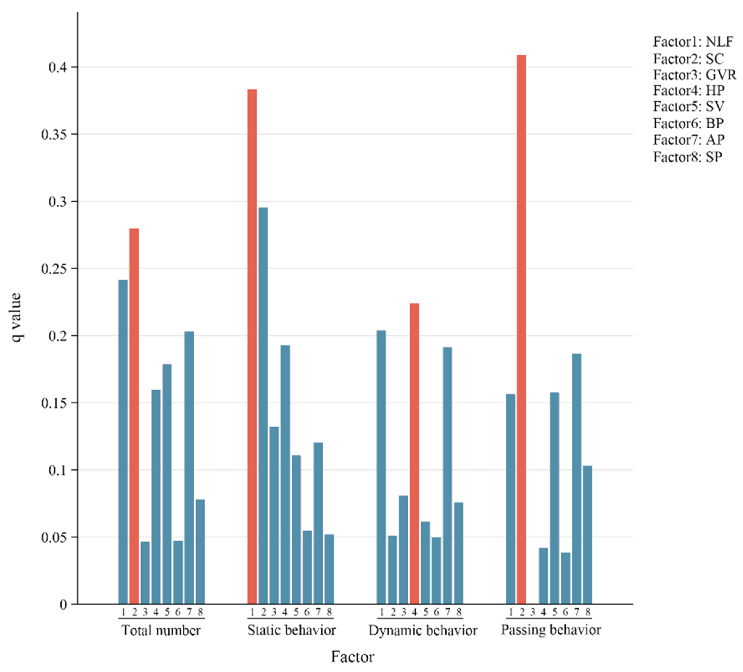
| NLF | 0.305223 | 0.19159 | 0.241322 | 0.383413 | 0.203616 | 0.156245 |
| SC | 0.167488 | 0.128352 | 0.279607 | 0.295082 | 0.050766 | 0.408536 |
| GVR | 0.166849 | 0.132109 | 0.046521 | 0.132047 | 0.080607 | 0.000581 |
| HP | 0.323279 | 0.279227 | 0.1598 | 0.192634 | 0.224013 | 0.041819 |
| SV | 0.151975 | 0.140865 | 0.178616 | 0.110659 | 0.061234 | 0.157544 |
| BP | 0.012177 | 0.02718 | 0.047045 | 0.05449 | 0.049493 | 0.038515 |
| AP | 0.198535 | 0.168921 | 0.202913 | 0.120521 | 0.191272 | 0.186338 |
| SP | 0.032529 | 0.012226 | 0.078083 | 0.051718 | 0.075686 | 0.102993 |
| Factors | BDI | BDO |
|---|---|---|
| NLF | 0.305223 | 0.19159 |
| SC | 0.167488 | 0.128352 |
| GVR | 0.166849 | 0.132109 |
| HP | 0.323279 | 0.279227 |
| SV | 0.151975 | 0.140865 |
| BP | 0.012177 | 0.02718 |
| AP | 0.198535 | 0.168921 |
| SP | 0.032529 | 0.012226 |
Disclaimer/Publisher’s Note: The statements, opinions and data contained in all publications are solely those of the individual author(s) and contributor(s) and not of MDPI and/or the editor(s). MDPI and/or the editor(s) disclaim responsibility for any injury to people or property resulting from any ideas, methods, instructions or products referred to in the content. |
© 2024 by the authors. Licensee MDPI, Basel, Switzerland. This article is an open access article distributed under the terms and conditions of the Creative Commons Attribution (CC BY) license (https://creativecommons.org/licenses/by/4.0/).
Share and Cite
Fan, S.; Huang, J.; Gao, C.; Liu, Y.; Zhao, S.; Fang, W.; Ran, C.; Jin, J.; Fu, W. The Characteristics of Visitor Behavior and Driving Factors in Urban Mountain Parks: A Case Study of Fuzhou, China. Forests 2024, 15, 1519. https://doi.org/10.3390/f15091519
Fan S, Huang J, Gao C, Liu Y, Zhao S, Fang W, Ran C, Jin J, Fu W. The Characteristics of Visitor Behavior and Driving Factors in Urban Mountain Parks: A Case Study of Fuzhou, China. Forests. 2024; 15(9):1519. https://doi.org/10.3390/f15091519
Chicago/Turabian StyleFan, Shiyuan, Jingkai Huang, Chengfei Gao, Yuxiang Liu, Shuang Zhao, Wenqiang Fang, Chengyu Ran, Jiali Jin, and Weicong Fu. 2024. "The Characteristics of Visitor Behavior and Driving Factors in Urban Mountain Parks: A Case Study of Fuzhou, China" Forests 15, no. 9: 1519. https://doi.org/10.3390/f15091519