Abstract
Rubber is a perennial plant grown for natural rubber production, which is used in various global products. Ensuring the sustainability of rubber cultivation is crucial for smallholder farmers and economic development. Accurately predicting rubber yields is necessary to maintain price stability. Remote sensing technology is a valuable tool for collecting spatial data on a large scale. However, for smaller plots of land owned by smallholder farmers, it is necessary to process productivity estimates from high-resolution satellite data that are accurate and reliable. This study examines the impact of spatial factors on rubber yield and evaluates the technical suitability of using grouping analysis with the forest classification and regression (FCR) method. We developed a high-density variable using spatial data from rubber plots in close proximity to each other. Our approach incorporates eight environmental variables (proximity to streamlines, proximity to main river, soil drainage, slope, aspect, NDWI, NDVI, and precipitation) using an FCR model and GIS. We obtained a dataset of 1951 rubber yield locations, which we split into a training set (60%) for model development and a validation set (40%) for assessment using area under the curve (AUC) analysis. The results of the alternative FCR models indicate that Model 1 performs the best. It achieved the lowest root mean square error (RMSE) value of 19.15 kg/ha, the highest R-squared (R2) value (FCR) of 0.787, and also the highest R2 (OLS) value of 0.642. The AUC scores for Model 1, Model 2, and Model 3 were 0.792, 0.764, and 0.732, respectively. Overall, Model 4 exhibited the highest performance according to the AUC scores, while Model 3 performed the poorest with the lowest AUC score. Based on these findings, it can be concluded that Model 1 is the most effective in predicting FCR compared to the other alternative models.
1. Introduction
Rubber, scientifically known as Hevea brasiliensis, is a perennial plant cultivated for harvesting natural rubber [1]. In addition to its economic value, rubber plants play a crucial role in absorbing carbon dioxide stored in biomass [2]. Rubber plantations cover approximately 78% (9.2 million hectares) of the agricultural land in Southeast Asia, with Indonesia accounting for about 31% (3.67 million hectares) and Thailand for about 28% (3.23 million hectares) [3]. These plantations mainly flourish in tropical regions, and the average lifespan of this species ranges from 30 to 35 years. Rubber trees are being cut down for their timber. This has resulted in an annual clearance and replacement of approximately 3%–4% of the plantation area with a new generation of rubber trees [4,5]. Rubber cultivation has undergone significant changes over the past century. Initially, rubber trees were grown over large areas, but there has been a gradual shift towards smallholder agriculture [6]. As of 2018, smallholder farmers have emerged as the predominant contributors to the production of natural rubber in the majority of Southeast Asian nations. Presently, they represent over 75% of the global production of natural rubber. The prominent countries in the natural rubber industry include Thailand, Indonesia, Vietnam, India, China, and Malaysia. Collectively, these countries achieved an astounding production output of 14.33 million tons of natural rubber in 2018 [2]. Due to its tropical location, Thailand provides a favorable environment for rubber cultivation. In the past, rubber cultivation in Thailand was primarily concentrated in the southern and eastern regions. However, there has been a discernible decline in the rate of growth of rubber plantations, particularly in the southern region. The government has implemented a policy that allows farmers to replace unproductive land for rubber trees with oil palm or fruit trees. As a result, the rubber industry has experienced recent growth in the northeast region, where it was previously absent. This expansion highlights the substantial contribution of rubber as a vital cash crop to the Thai economy.
Natural rubber production holds immense significance for more than 20 million farmers globally. Over the course of the last century, the onus of rubber cultivation has increasingly shifted towards small-scale farmers, who currently account for over 75% of the total global natural rubber output. While the sizes of rubber plantations may differ across countries, it has been documented that the majority of small-scale farmers possess less than 4 hectares of land. Remarkably, these small-scale farmers consistently achieve impressive rates of natural rubber production, ranging from 85% to 93%. However, smallholder rubber farmers continue to encounter various challenges, such as insufficient income and limited access to financial resources. Therefore, it is imperative to establish sustainability in the production of natural rubber, specifically to promote the growth of the global economy.
Remote sensing technology is a highly valuable tool for collecting extensive amounts of spatial data [7,8,9,10,11]. Satellite imagery is particularly useful because it is freely available, covers wide geographic areas, and has high temporal resolution. In the case of rubber plantations, satellite images with multiple spectra can be used to identify harvesting areas using different photo indices [12]. Technology plays a pivotal role in the accurate mapping of rubber plantations at both the local and regional levels [13,14,15]. Furthermore, remote survey tools facilitate real-time monitoring of any modifications that take place in rubber plantation areas. This not only obviates the need for laborious and costly field inspections but also permits potential access restrictions [16,17]. Yield estimation is of paramount importance in maintaining price stability, and numerous countries rely on commonly employed techniques such as yield data collection and field-based reports. However, it is worth noting that a significant proportion of these methods heavily depend on relatively time-consuming post-harvest surveys [18]. Remote sensing using satellites can serve as an alternative approach for the estimation and prediction of agricultural yield. This area of research is of great importance [19] and forms a crucial component of assessing and forecasting agricultural yields [2,20]. Several studies have utilized vegetation indices derived from remote sensing data to estimate crop yields in various crops, including rice, wheat, barley [20,21,22,23,24], potato [25,26,27], maize [28,29,30,31,32], and oil palm [33,34,35,36]. Remote sensing technology in agriculture, particularly in yield estimation and crop forecasting, is a critical area of research [37,38]. Several studies have utilized low-resolution MODIS satellites to effectively address the classification challenge. These studies have made use of biophysical properties derived from time-series data, yielding encouraging outcomes [14,39]. The Landsat satellites, known for their moderate spatial resolution of 30 m, have been successfully utilized to estimate the growth and age of rubber trees [40,41,42]. The THEOS satellite was used to analyze changes and expansions in rubber plantation areas in northeastern Thailand. However, most studies relied on low-resolution MODIS data, and only one study utilized THEOS satellite data for tire yield applications. Satellite data are commonly used in the rubber industry but are ineffective in accurately assessing rubber yields due to their limited spatial resolution [43]. The Sentinel-2 satellites, known for their high resolution, can differentiate between rubber plantations and intricate natural forests [44,45]. Sentinel-2A and Sentinel-2B work together to provide high temporal and optimum spatial resolutions. This makes them ideal for continuous monitoring and small-area coverage [46]. Previous research has primarily focused on increasing natural rubber production in large areas, neglecting the challenges faced by smallholder primary producers.
Remote sensing information systems are an invaluable resource for the geographical study of rubber yield. Geographic Information System (GIS) expertise serves as a highly effective analytical tool in this field. Satellite imagery, obtained through remote sensing (RS), enables a comprehensive analysis of latex rubber yield. This analysis can encompass a wide range of indicators, such as the standardized vegetation index, the soil moisture index, and the soil cover index, in addition to spatial factors that are intricately linked to rubber production. Previous studies by [47,48,49,50] have employed spatial statistics to explore the geographical factors that correlate with rubber yield. However, these studies analyzed large areas, resulting in inconsistencies and discrepancies in the raster data. To address this issue, GWR (geographic weighted regression) models were developed for hydrological factor analysis, focusing on small-area unit systems. These models have proven effective, with high R2 values observed across all models [47]. By combining spatial modeling with mathematical models, the accuracy of linear models and yield prediction can be enhanced. However, when using spatial statistical models for forecasting, risk analysis is limited to the level of the sub-basin. In order to generate relevant trendlines, it is crucial to have enough independent variable data. Therefore, by incorporating machine learning (ML) and leveraging spatial characteristics, it becomes possible to estimate rubber yield in specific water supply locations.
Machine learning (ML) has been used in modern research to perform spatial risk assessment tasks, as discussed in [51]. In recent years, there have been significant advancements in ML algorithms, computing power, and geospatial innovations, such as software. These developments have greatly simplified the process of creating spatial maps [52]. Recent papers have presented machine learning algorithms, including knowledge-based methods [53], multivariate logistic regression methods [54,55,56], and multivariate binary logistic regression methods [57], as effective tools for enhancing the accuracy of spatial maps. Additionally, various other methods, including general linear models [58,59], quadratic discriminant analysis [49,60], boosted regression trees [59,61], random forest classification (RFC) [62,63,64,65], multivariate adaptive regression splines [66,67], classification and regression trees [59,68], support vector machines [69,70,71], naïve Bayes [72,73], generalized additive models [58,68], neuro-fuzzy and adaptive neuro-fuzzy inference [74,75,76], fuzzy logic [77], artificial neural networks [78,79,80,81,82,83], maximum entropy [84,85], and decision trees [86,87], have also been presented. ML applications are commonly used to create landslide maps (LSM). According to Merghadi et al. [88], tree-based ensemble optimization algorithms are more effective than other ML algorithms. In a comparative analysis conducted by Sahin [89], Catboost was found to have the highest precision (85%), followed by XGBoost (83.36%). Catboost also demonstrated more accurate prediction of sample proportions compared to other models. The main advantages of ML and probabilistic processes include their objective statistical foundation, repeatability, ability to quantitatively analyze the impact of variables on spatial prediction, and the potential for regular updates. During the review of different machine learning approaches for predicting agricultural output, it was discovered that the random forest classification (RFC) technique consistently provided accurate results in numerous tests. Therefore, for this study, a random forest model in the form of the forest classification and regression (FCR) function within the ArcGIS program, which is widely used for geographic information analysis, was chosen as the primary tool for conducting the research.
There is a scarcity of research on rubber yield in small river basins, particularly regarding the influence of spatial factors. Currently, there is no existing direct model for predicting rubber yield in areas adjacent to major rivers such as the Mekong River. This study proposes the utilization of spatial features as indicators of rubber yield through the application of the FCR modeling technique. The primary objective of this study was to identify the key features of small river basins that have the most significant impact on variations in rubber yield. These identified characteristics were then utilized to develop a forecasting model based on FCR. This research holds the distinction of being the first to apply FCR in predicting rubber yield within this specific context, setting it apart from previous studies.
The previous study utilized FCR methodologies to predict rubber yield by analyzing spatial parameters at the watershed level and learning from specific rubber parcels. This approach enables effective management of training clustering points for accurate predictions, as long as the spatial distribution of each parcel’s features remains significant within each sub-basin unit [90]. However, this method requires estimation methods from point data to match the grid size, which may introduce multicollinearity—a correlation between independent variables—due to data increase or decrease.
2. Materials and Methods
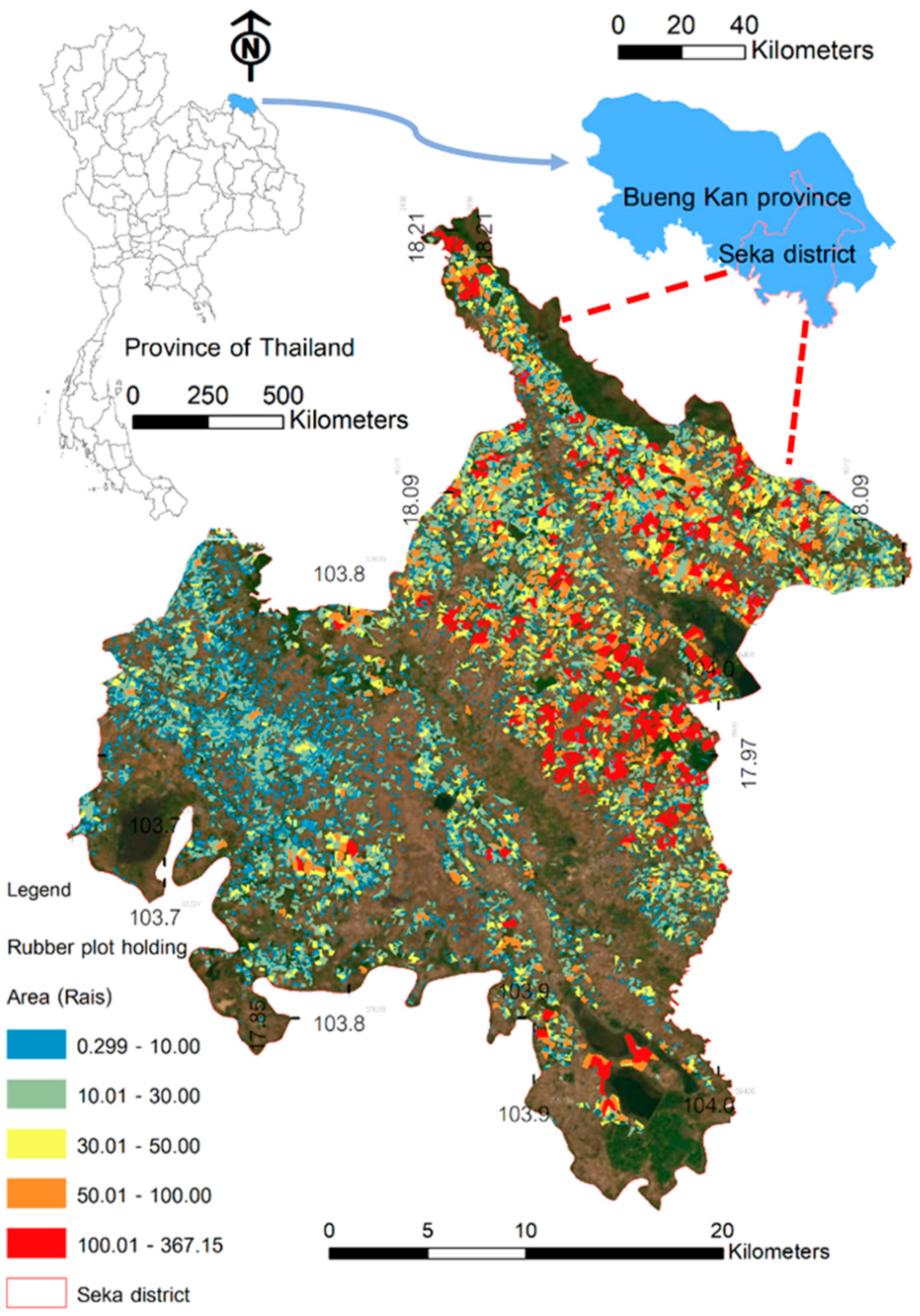
The study was conducted in the Seka district of Bueng Kan Province, situated in the upper northeast region of Thailand. Bueng Kan Province has geographical coordinates ranging from 17°46′ to 18°26′ N and 103°14′ to 104°11′. Renowned for its favorable conditions for rubber cultivation, Bueng Kan is the ninth largest area for rubber plantations in Thailand and is home to the largest rubber plantation in northeastern Thailand. The province covers a total area of 2,777,570 rai (444,411.2 hectares), with a rubber plantation area of up to 1,198,965.45 rai (191,834.472 hectares). This equates to approximately 4300 km2 of lowlands (refer to Figure 1). The region experiences a favorable climate, with an average temperature of 27 °C and annual rainfall ranging between 1500 and 2500 mm. The terrain predominantly consists of plateaus. Classified as tropical and characterized by dry rain, the climate in the Seka district is particularly suitable for rubber cultivation. Consequently, it is one of the districts in Bueng Kan Province where rubber cultivation is preferred by the majority of the population over other agricultural crops.

Figure 1.
The study area: Bueng kan Province and the Seka district.
Rubber plantations cover the largest expanse, totaling 775,994 rai (124,159.04 hectares), which accounts for 59.90% of the overall cultivated area. Seasonal rice covers 492,181 rai (78,748.96 hectares), representing 38% of the total cultivated area. Oil palm occupies 14,184 rai (2269.44 hectares), making up 1.09% of the cultivated area, while off-season rice covers 13,030 rai (2084.8 hectares), accounting for 1.01% of the total cultivated area (Office of Agricultural Economics 2014). In the study area, most of the rubber plant species planted were RRIM 600, and the typical plantations in the area range from 5 to 30 rai in size. Seka District in Bueng Kan Province is an ideal location for rubber cultivation due to its humid climate, adequate rainfall, and loam soil that is well-suited for growing rubber trees. These factors not only prevent the plants from withering but also promote fast root growth. Ultimately, this will result in robust rubber tree growth and a high yield in the future.
2.1. Spatial Factors
The FCR model utilized in this study incorporates nine spatial factors that are linked to tire yield percentages. These factors include the index of land use type, soil drainage, road networks, and the proximity to surface water sources. In this study, an independent set of variables was reconstructed within a grid size of 10 m × 10 m to accurately describe the data values of all the variables. Border distances were defined using distance analysis variables. The mathematical model was adjusted to fit the grid, and the score values of the independent variables were obtained from data provided by the Rubber Authority of Thailand (RAOT). Based on previous research, this study identified the following guidelines for implementing the model: A machine learning model using FCR was developed to analyze the spatial factors associated with rubber yield. The study had two objectives: (1) to analyze the spatial factors that are correlated with rubber yield and (2) to predict rubber yield using a machine learning-based FCR model. The purpose of this study was to develop a set of independent variables for predicting rubber production based on spatial factors. The chosen prototype area was suitable for cultivating rubber under controlled conditions similar to other variables. Our study aimed to evaluate physical factors that may impact yield and reduce the number of variables from 8 to a more representative set for an alternative model. This was achieved through an analysis of spatial correlations.
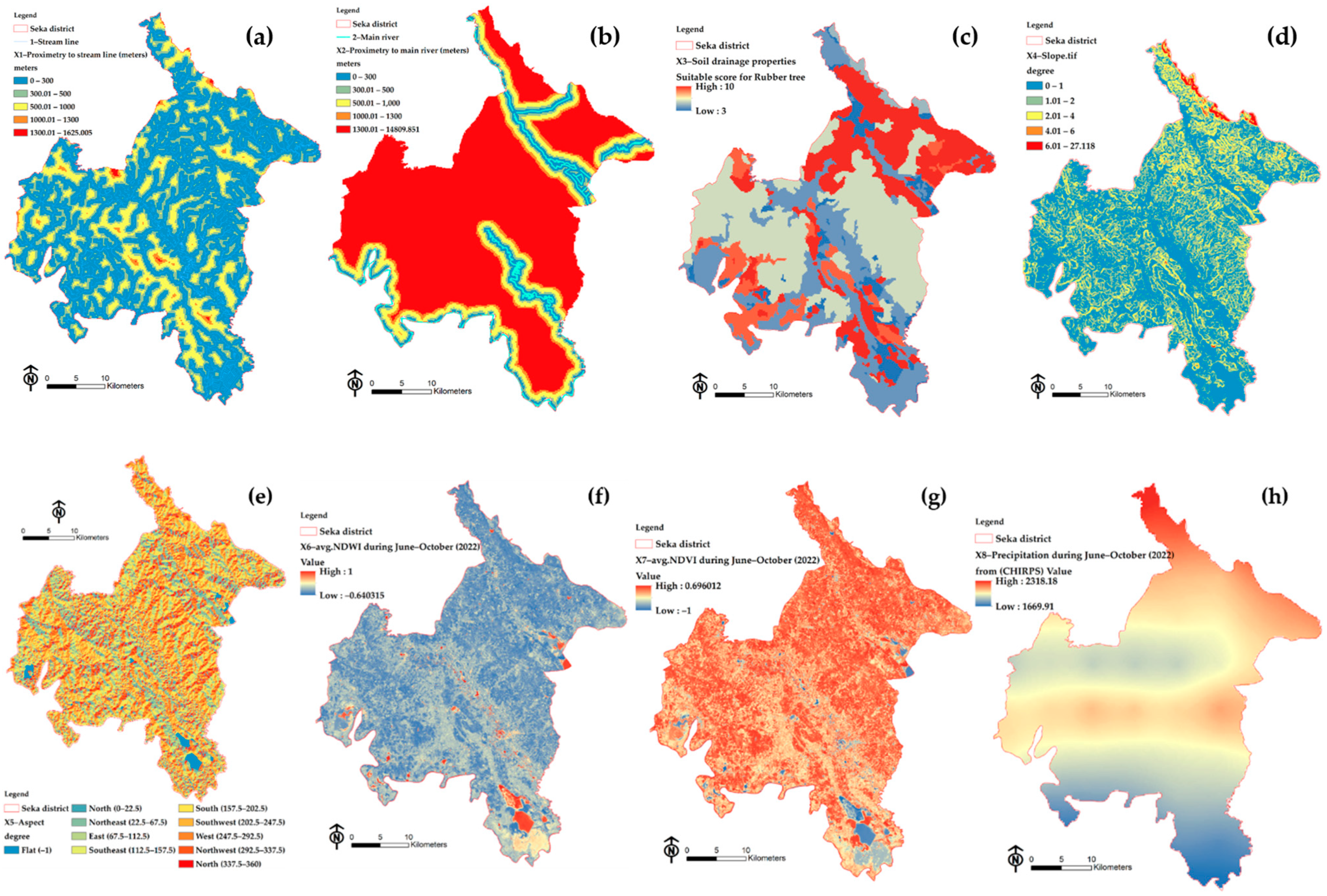
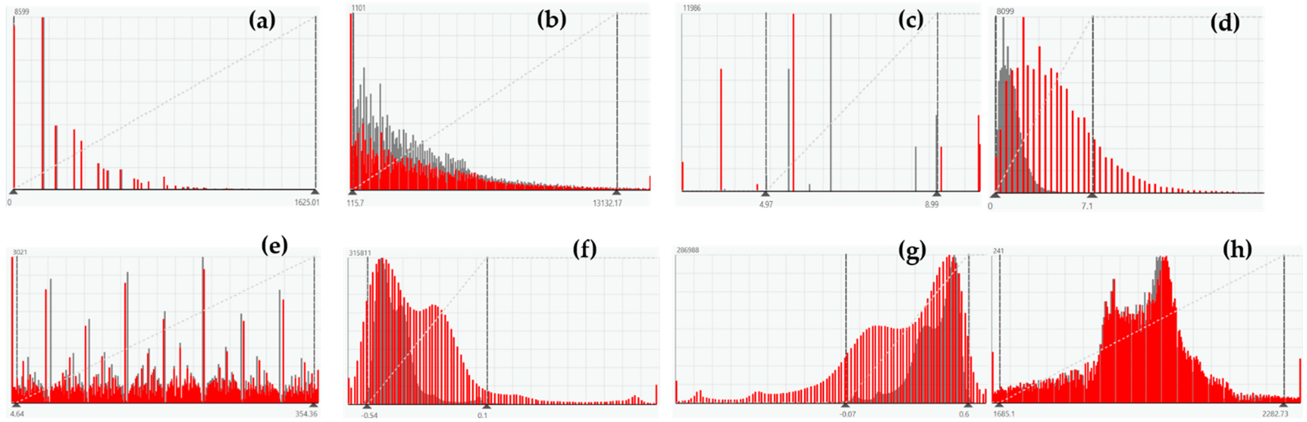
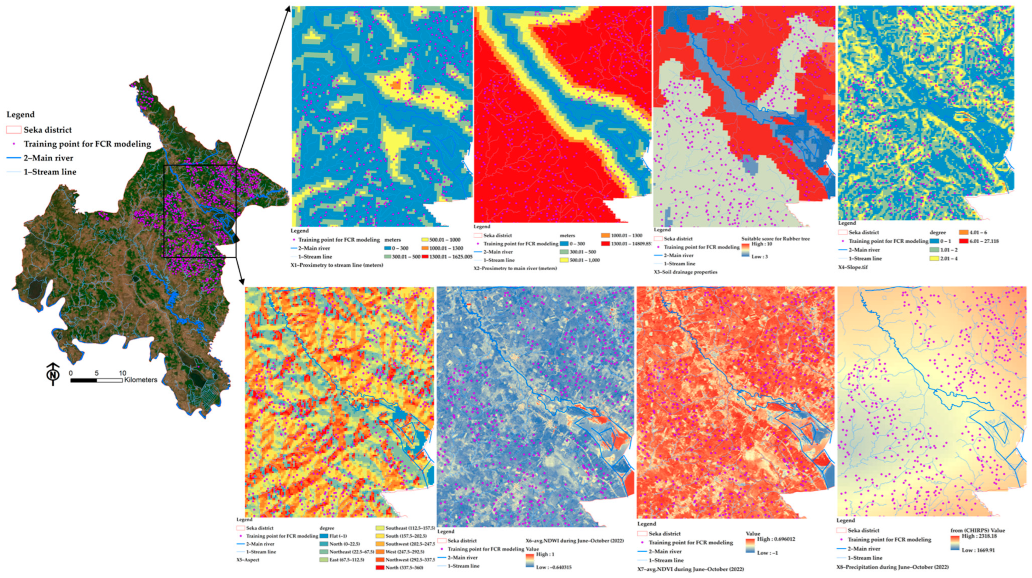
The set of independent variable factors included both spatial factors and remote perception index factors [91]. In the first test, these factors were divided into two cases, one of which used grid-specific attribute values as learning agents. Figure 2 depicts the map for each factor, and histograms are displayed in Figure 3.
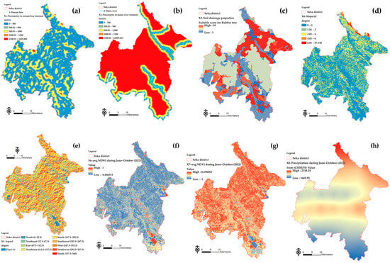
Figure 2.
Criterion maps of spatial factors for FCR modeling: (a) X1, (b) X2, (c) X3, (d) X4, (e) X5, (f) X6, (g) X7, and (h) X8.
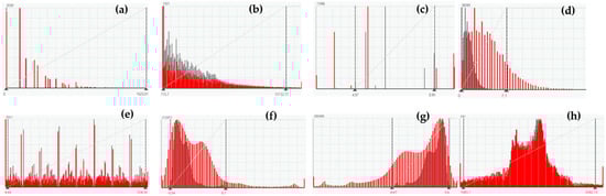
Figure 3.
Histograms of spatial factors: (a) X1, (b) X2, (c) X3, (d) X4, (e) X5, (f) X6, (g) X7, and (h) X8.
2.1.1. Proximity to Streamlines (X1)
The presence of a significant water source nearby has a significant impact on rubber production in the following areas: Watering: Having a nearby water source makes it easier to water rubber trees, which directly affects their growth and leads to greater yields. Humidity control: The availability of nearby water sources also plays a crucial role in controlling soil moisture in rubber growing areas. This ensures that the rubber trees receive the optimal amount of water for their growth. Growth: A significant water source nearby greatly aids in the growth of rubber trees, ultimately affecting the quantity and quality of the rubber produced. Therefore, it is imperative to have a significant water source nearby in order to efficiently produce rubber of the highest quality.
2.1.2. Proximity to Main River (X2)
Planting rubber trees in close proximity to major rivers has resulted in a significant boost in rubber yields. This can be attributed to the invaluable contribution of rivers in providing a substantial water source for optimal rubber growth. Additionally, the availability of an ample water supply further augments the delivery of essential nutrients to the rubber trees, resulting in higher quality and more efficient tire production. Furthermore, locating rubber plantations near rivers helps to regulate the temperature in the area, ensuring optimal conditions for the growth of rubber trees.
2.1.3. Soil Drainage (X3)
The growth of rubber trees depends on the soil’s drainage properties. When the soil has high porosity, it allows the roots of the rubber trees to penetrate easily. This helps with the absorption of water and nutrients, resulting in better growth. Additionally, the drainage properties of the soil affect the drainage and moisture control of rubber plantations. Well-drained soil reduces the risk of waterlogging and the buildup of harmful pathogens. It is therefore important to choose soil with excellent drainage for optimal rubber tree growth and efficient yield production.
2.1.4. Slope (X4)
The slope of the rubber growing area has a significant impact on rubber yield. A steep slope can cause rainwater to flow rapidly, resulting in uneven seepage into rubber tree roots. Insufficient water absorption in the tree hampers the development of synthetic substances and the overall growth of rubber trees.
2.1.5. Aspect (X5)
These factors have a direct impact on the growth of rubber trees and the synthesis of food in plants. When a rubber tree is exposed to sufficient light, it adjusts to optimize the intake of light waves during its initial development. The process of cell division is enhanced, facilitating effective external and internal tracking of rubber pressure. As a result, pressure transfer becomes faster and power escape is minimized. This leads to the production of high-quality rubber with a high yield. It is observed that the best direction for optimal rubber yield is when the rubber plantation is situated perpendicular to the east–west axis.
2.1.6. NDWI (X6)
NDWI (the Normalized Difference Water Index) is a widely utilized metric for assessing soil moisture and canopy water content. This index operates by analyzing the interaction between water molecules present in the canopy and sunlight [52]. It is influenced by regional climate and soil characteristics which impact water availability, and it is highly responsive to alterations in liquid water [53]. The NDWI derived from Sentinel-2 utilizes two near-infrared channels, each with a spatial resolution of 10 m. The purpose of calculating NDWI is to identify discrepancies in color levels between dry and watery substances within imagery data. The process involves the following steps: NDWI = (Green Band − NIR Band)/(Green Band + NIR Band). The green band represents the color value within the green range, while the NIR band represents the color value in the spectrum near bright colors. The NIR band can be used to identify various elements nearby, such as water and heat. By analyzing and monitoring water status in different areas, this index helps make accurate predictions about future water conditions.
2.1.7. NDVI (X7)
The Normalized Difference Vegetation Index (NDVI) is widely regarded as the most suitable index for global vegetation monitoring through satellite data. This index is particularly advantageous, as it incorporates variations in lighting conditions, surface slope, exposure, and other external factors [40]. This index is calculated using the near-infrared (NIR) and red bands. Sentinel-2 calculates NDVI by utilizing wavelengths found in the red and near-infrared spectra. Specifically, the red band covers a range of about 0.64–0.68 μm, whereas the near-infrared band spans approximately 0.78–0.90 μm. Through the comparison of reflectance values in these two bands, NDVI can be computed to evaluate the health and density of vegetation.
2.1.8. Precipitation (X8)
The yield of rubber is consistently affected by rainfall due to its impact on the growth of rubber trees. Adequate rainfall promotes good growth, leading to increased latex formation and higher rubber production. However, excessive rainfall can be detrimental to rubber trees, causing their deterioration and reducing yield. Therefore, it is crucial to properly manage rainfall to ensure effective rubber production.
2.2. Clustering Analysis for Training Point Selection
Clustering analysis is a helpful technique for grouping data. It involves using the cluster method to group data that have similar amounts of rubber yield. This method focuses on the similarity of data within the same group and the differences between groups. By grouping data, we are able to understand the relationships between different data points and analyze them efficiently. There are various methods available for data grouping, such as K-means clustering, hierarchical clustering, and Getis–Ord. Each clustering method possesses unique advantages and disadvantages. Therefore, it is essential to meticulously choose a clustering method that aligns with the specific data and analysis objectives. In this study, our methodology enabled the analysis and categorization of data within the same group to create FCR models and accuracy test sets. The data groups utilized for machine learning were classified using the clustering method, as illustrated in the enlarged image in Figure 4.
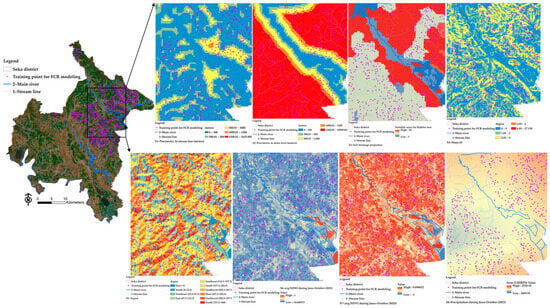
Figure 4.
The example of clustering of training points (hot spots > 90% confidence) for FCR modeling.
2.3. Predicting Rubber Yield
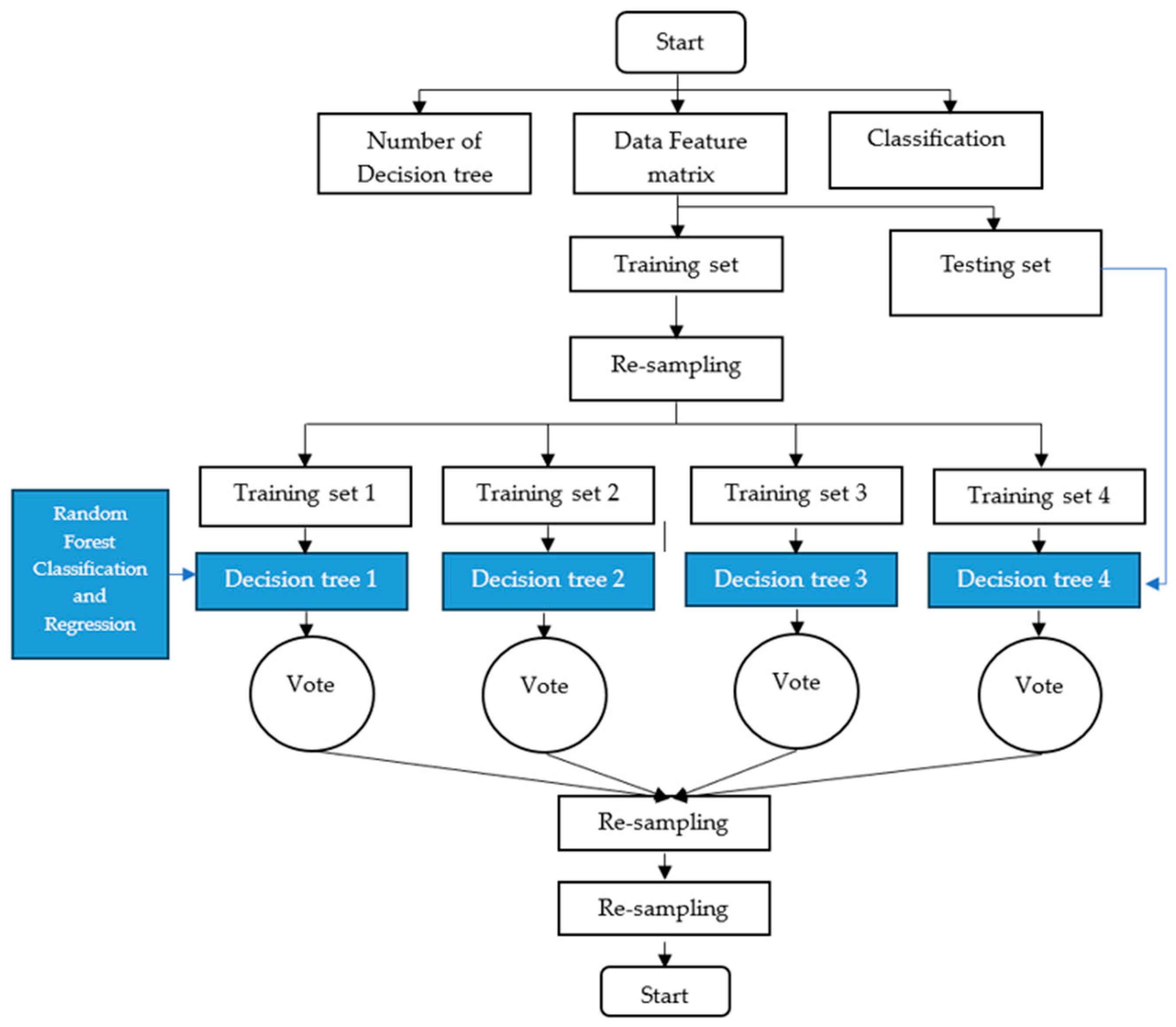
The model utilized in this study was designed to assess the accuracy of rubber yield prediction per rubber plot in a specific region. However, the aim of this study was to evaluate the extent to which the independent variable set employed could enhance the predictive capability of rubber yield. The random forest (RF) algorithm, introduced by Leo Breiman in 2001, is a highly regarded algorithm in the field of machine learning [92] and a popular ensemble technique in supervised machine learning. It can be used for both classification and regression tasks. Known for its reliability, RF is able to make accurate predictions even with large datasets, as it is resistant to overfitting. This system has the ability to handle a significant volume of input features and assess the predictive strength of all variables [92,93]. RF operates by generating an ensemble of diverse trees, each derived from bootstrap samples [94]. The model uses “in-bag” data for training and “out-of-bag” data for validation. Generally, two-thirds of the bootstrap samples are used for training. To enhance prediction accuracy and maximize the model’s effectiveness, it is crucial to optimize two factors: the number of trees generated (ntree) and the number of splitable parameters at each tree node (mtry), as suggested by Taalab et al. [95]. Extensive research, both theoretical and empirical, has demonstrated the many advantages of RF models. These models are highly regarded for their ability to accurately forecast, handle outliers and noise, and avoid overfitting. Because of these strengths, RF shows great potential in assessing flood hazard risks, especially when confronted with intricate challenges that involve multiple variables and non-linear dynamics [96]. Unlike traditional methods such as bagging, RF structures can effectively decrease the attributes in each decision tree (DT), resulting in greater variability between DTs and addressing the curse of dimensionality [97]. The RF model is capable of accurately capturing the complexities involved in predicting agricultural yields by considering non-linear relationships and interactions among various factors. Furthermore, the ensemble learning technique employed by RF enables it to effectively combine information from multiple decision trees, resulting in improved prediction accuracy and reduced bias and variance. Lastly, RF’s scalability and ability to handle large datasets make it an indispensable tool for predicting rubber yields, which often requires analyzing extensive spatial and remote sensing data. The RF process commences with a decision tree structure, commencing with a sample input and branching out according to pre-established criteria. In the event that the criteria are satisfied (“yes”), the decision tree proceeds along the predefined route. Conversely, if the criteria are not satisfied (“no”), an alternative route is taken. This iterative process persists until the decision tree ultimately reaches a terminal node, which ultimately determines the final outcome (Figure 5). Figure 5 explains how the forest-based classification and regression tool trains a model using known values from a training dataset. This model can then be used to predict unknown yield values in a prediction dataset with the same explanatory variables. The tool uses the random forest algorithm to create multiple decision trees, referred to as an ensemble or a forest, for prediction. Each tree generates its own prediction, and these predictions are combined using a voting scheme to make the final predictions. The final predictions are not based on a single tree, but rather on the entire forest. This approach helps avoid overfitting the model to the training dataset by using a random subset of the training data and a random subset of explanatory variables in each tree of the forest.
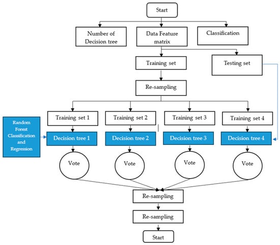
Figure 5.
The structural framework of random forest classification and regression.
We utilized ArcGIS Pro (v3.2.0) to analyze the forest classification and regression model (FCR) for this research. Initially, we resampled the eleven environmental variables to a spatial resolution of 10 m using raster map algebra. Subsequently, we transferred the data from each pixel to the FCR tool, while also incorporating corresponding rubber yield data into the model. Sixty percent of the data were allocated for model training. The remaining portion was used for model validation. The model was subsequently fine-tuned to identify the optimal values for two crucial factors: the number of trees (ntree) and the maximum number of nodes in each tree (maxnodes). In this study, we utilized the RMSE and R2 metrics to assess the efficacy of machine learning models for both classification and regression tasks. Equations (1) and (2) present the mathematical formulations for the aforementioned metrics, respectively. Equation (1) visually demonstrates the fluctuations of RMSE with changes in ntree and maxnodes. According to our estimations, we determined that the ideal quantity of trees was 1000, with a maximum node count of 70 for each tree.
To use the Random Forest Regression algorithm in ArcGIS Pro v3.20 software, follow these three steps: 1. Generate multiple models using the random forest approach, typically ranging from 10 to over 1000 models. 2. Each model is trained on a unique dataset, which is a subset of the complete dataset. When making predictions, every decision tree within the random forest provides a forecast for the dataset being analyzed. The final prediction is determined through a process of voting for the most preferred output in classification or by calculating the average of all decision tree outputs in regression. In order to train a model using the FCR tool, a training dataset containing known values, such as average attributes on a grid, is necessary. Once the model is trained, it can be applied to forecast unknown values by utilizing a prediction dataset that shares the same independent variables. ArcGIS Pro utilizes Leo Breiman’s random forest algorithm [98], a supervised machine learning technique, to build models and generate predictions. For this study, the FCR tool was employed.
- Pre-processing
Each decision tree model within the random forest is regarded as a weak learner, indicating that its individual predictive power is not particularly robust. However, when these decision trees are aggregated to collectively make predictions, users obtain a comprehensive model that surpasses the accuracy of a single decision tree in isolation.
- Dimensions of the dataset in a random forest
Each decision tree model is regarded as a weak learner, indicating that its independent effectiveness is limited. Nevertheless, when these decision trees collaborate to make predictions, the resulting model becomes stronger and more accurate than a solitary decision tree making an individual prediction.
- Feature selection
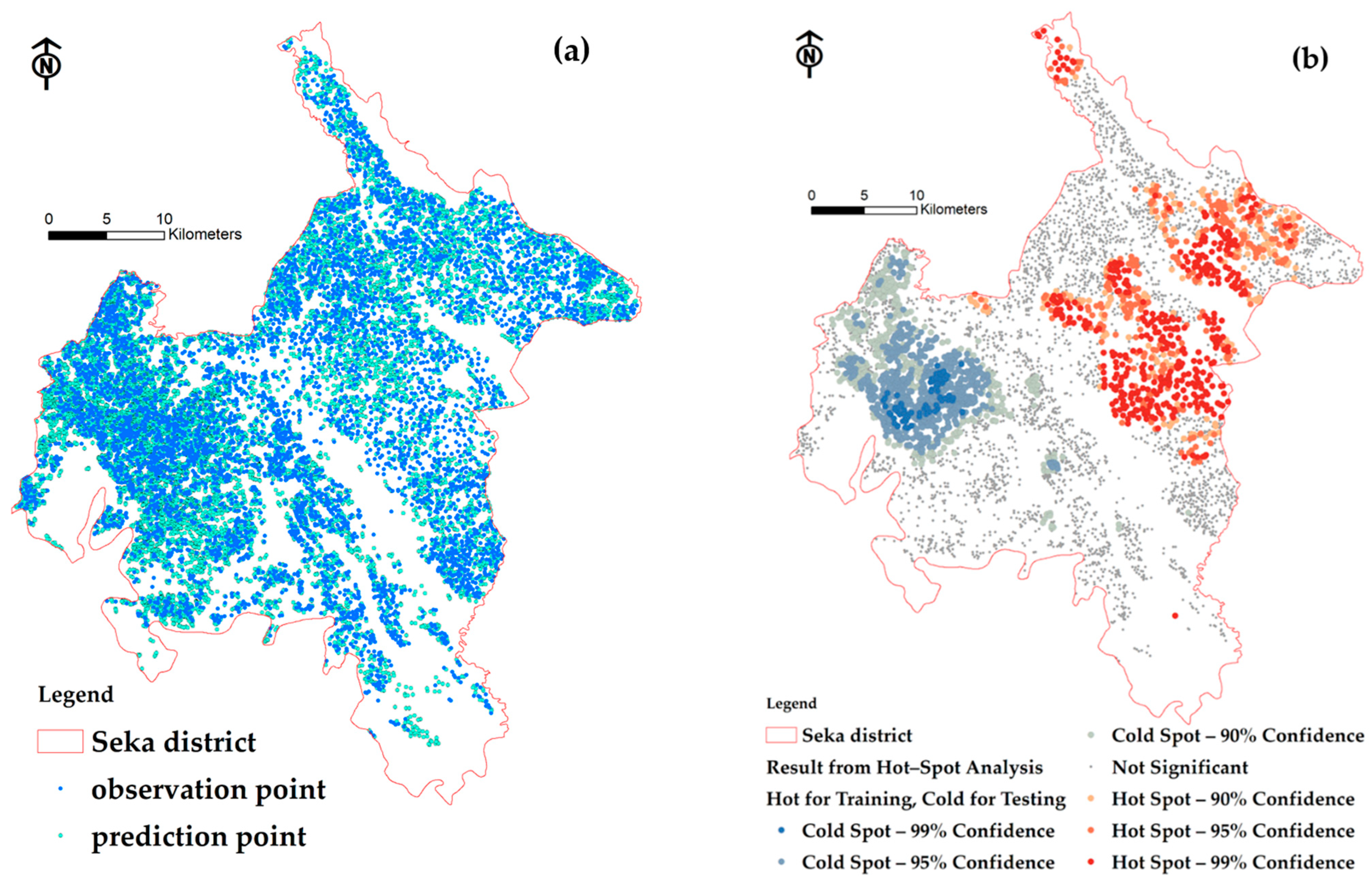
All datasets were both trained and tested. Within the survey grids conducted in 1951, rubber yield parcels were identified. These parcels consisted of 847 modeling points and 1104 testing points, as shown in Figure 6a,b. The point at which the yield grouping value surpasses the mean value, as indicated by the hot-spot index, serves as the learning point for the FCR model. Conversely, the point within the group with a rubber yield lower than the average, depicted in blue or referred to as the cold-spot value, is used as the accuracy test point for the FCR model.
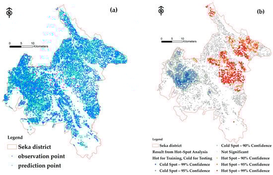
Figure 6.
The observation points and prediction points of rubber parcels: (a) total rubber parcels; (b) the results of the rubber yield grouping using the Getis–Ord method reveal a cluster of data points with overlapping yield values surpassing the average value represented in red, while yield values below the average are represented in blue.
To maintain data sampling integrity and impartiality, repeated sampling was conducted over 300 runs using the standard FCR model settings. The learning parameters included 300 trees, a tree depth range of 9 to 31, and a leaf size of 5. The forecasting model integration employed a boosting strategy, which involved developing multiple data categorization models. Each model in this study was constructed using the same training data but with an extra weighted value [99]. To assign new data groups, weighted voting methods were employed, with two specific methods used: average and weighted voting.
To assess the accuracy of the RF algorithm, we used the commonly applied receiver operating characteristic–area under the curve (ROC–AUC) technique. This technique is widely used in machine learning to evaluate model performance and address interpretation and criteria selection concerns [100]. ROC curves are created by plotting the true-positive rate (TPR), also referred to as sensitivity, against the false-positive rate (FPR), which represents specificity [99]. The TPR on the y-axis measures the proportion of true positives correctly identified, while the FPR on the x-axis measures the proportion of false positives or negative instances incorrectly classified as positive. Additionally, the ROC curve provides insight into the frequency at which the model incorrectly predicts a positive outcome when the actual outcome is negative. Equations (1) and (2) can be used to calculate the TPR and FPR.
TP represents the number of correctly predicted positive instances, FN represents the number of positive instances that were incorrectly predicted as negative, FP represents the number of negative instances that were incorrectly predicted as positive, and TN represents the number of correctly predicted negative instances. Calculating the true-positive rate (TPR) and false-positive rate (FPR), an area under the curve (AUC) value of 50% indicates that the estimation lacks discrimination. Conversely, if the AUC exceeds 90%, the model is considered to have exceptional predictive power [98].
3. Results
3.1. Correlation Analysis and Dendrogram
Based on the correlation data between the eight given variables, as shown in Figure 7, the following observations can be made: Variable X2 (prox2mainriver) has a positive correlation with variable X1 (prox2stream) at a level of 0.039, with a coefficient less than 1. Variable X3 (soil drainage) has a negative correlation with variable X2 (prox2mainriver) at −0.273 and a positive correlation with variable X1 (prox2stream) at a level of 0.042, both with coefficients less than 1. The variable X5 (aspect) has a positive correlation with the variables X4 (slope) and X2 (prox2mainriver) at levels of 0.983 and 0.009, respectively, both with coefficients similar to 1. The variable X7 (NDVI) has a negative correlation with the variable X6 (NDWI) at a level of −0.967 and with the variable X4 (slope), with a coefficient close to −1. The variable X8 (precipitation) has a positive correlation with the variables X4 (slope) and X5 (aspect) at levels of 0.688 and 0.676, respectively, both with coefficients close to 1. When analyzing individual variables, X2, X3, X5, X7, and X8 are suitable for modeling due to their coefficients being close to 1 or −1. This indicates a clear relationship between these variables and others, allowing for the creation of more accurate and reliable models. On the other hand, the X1 and X6 variables are not suitable for modeling as their coefficients are less than 1 and not close to 1 or −1. This suggests an unclear relationship between these variables and others, which can result in modeling inaccuracies and unreliable results.
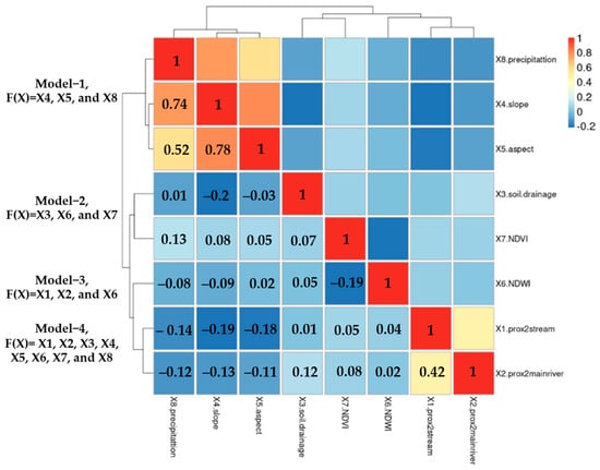
Figure 7.
Correlation matrix of alternative model for testing spatial factors on rubber yield.
The test was divided into six sub-models based on spatial correlation analysis. Model 1 included X4 and X8, while Model 2 combined these variables into one data layer using X5. Alternative Models 3 and 4 followed a similar approach but with different independent variables: X3 and X7. Model 5 and Model 6 specifically incorporated X1, X2, and X6 as independent variables. The segmentation approaches were analyzed through the dendrogram graph, which enabled a clear comparison and effective selection of the appropriate set of variables to import into the FCR model.
3.2. Predicting Rubber Yield Using a Machine Learning-Based FCR Model
Table 1 presents the results of the FCR model, which uses integers ranging from two to five with one decimal place. The model includes the following factors for interpretation: (1) Number of Trees: This indicates the total number of trees in the model, set at 300. (2) Leaf Size: This refers to the size of the leaves within the tree, set at 5. (3) Tree Depth Range: This represents the range of depths for the trees, which falls between 17 and 33. (4) Mean Tree Depth: This indicates the average depth across all trees created, set at 22. (5) % of Training Data Available per Tree: This reflects the percentage of training data used to build each individual tree, set at 100%. (6) Number of Randomly Sampled Variables: This refers to the number of randomly generated variables in each tree, set at 2. (7) % of Training Data Eliminated for Validation: This represents the percentage of training data, specifically 10%, that are removed for model testing purposes.

Table 1.
Model characteristics.
In the case of 50 trees, the mean square error (MSE) is 758.876, indicating a high prediction error. The percentage of variation explained is −25.169%, meaning that the MSE obtained using the random forest model with 50 trees can only account for 74.831% of the variance. For the case of 100 trees, the MSE value obtained is 702.985, indicating a lower tolerance. The percentage of variation explained is −15.951%, indicating that the MSE obtained using the random forest model with 100 trees can explain the variability of the data. Compared to using 50 trees, it has a more favorable effect, returning to the prediction.
Each decision tree in an FCR is trained using a subset of the training data and a randomly selected subset of features. (More details can be found in Table 2). This approach mitigates the risk of overfitting and improves the model’s capacity to generalize. The significance of each variable in the FCR model is assessed based on its contribution to the overall model performance. Variables with higher importance values exert a more substantial impact on the model’s predictions. Table 3 displays the importance of each variable in the random forest model. For instance, variable X2 has the highest importance value of 79,633.31, indicating its significant role in the model’s performance. Similarly, variables X5, X4, X8, X6, and X7 also have high importance values, while variables X1 and X3 have lower importance values. The most important variable in the FCR model is X2, with an importance value of 79,633.31, representing a 15% impact on the results. Following closely are variables X5, X4, X8, X6, and X7, all with equal importance values of 15%. The X1 variable has a 9% importance, while the X3 variable has the least importance at only 3%. Consequently, when analyzing the data, it is advisable to prioritize the use of variables X2, X5, X4, X8, X6, X7, and X1 over variable X3.
Table 2.
Model out-of-bag errors.
Table 3.
Top variable importance.
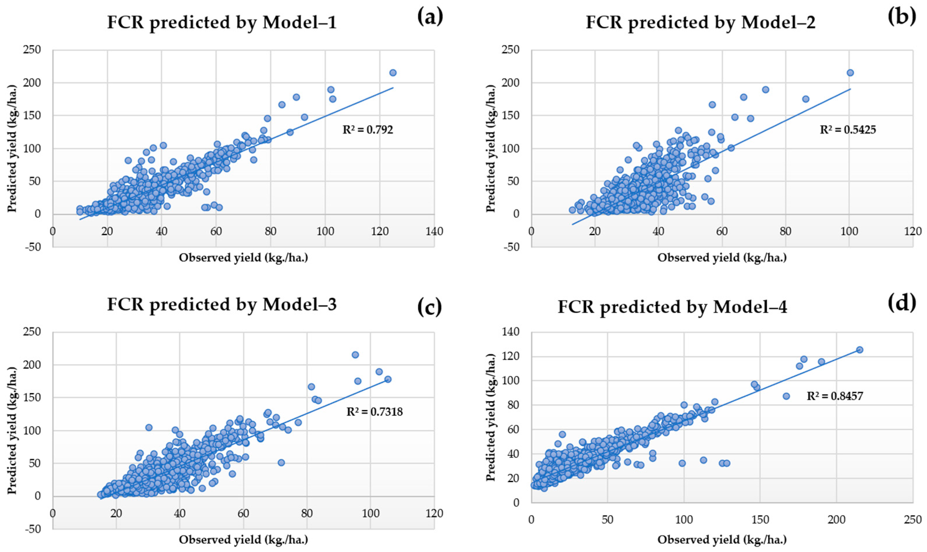
According to the analysis, Model 4, which utilized Factors X1, X2, X3, X4, X5, X6, X7, and X8, demonstrated the lowest RMSE of 15.87 kg/ha and the highest R2 (FCR) of 0.821, as displayed in Table 4. Additionally, Model 4 demonstrated an R2 value (OLS) of up to 0.678. When compared to other models, it was found that this model showed the highest correlation between primary and following variables in this clause. Therefore, Model 4 with Factors X1, X2, X3, X4, X5, X6, X7, and X8 is considered a suitable model for predicting rubber yields. When comparing the results of the three models presented in Figure 8, it is evident that Model 1 exhibits the best performance. It achieves the lowest RMSE value of 19.15 kg/ha, the highest R2 value (FCR) of 0.787, and also the highest R2 (OLS) value of 0.642. On the other hand, Model 2 has a higher RMSE than Model 1, measuring 28.97 kg/ha; an average R2 (FCR) of 0.542; and a highest R2 (OLS) value of 0.503. Finally, Model 3 demonstrates the highest RMSE of 30.26 kg/ha, the lowest R2 (FCR) of 0.730, and the highest R2 (OLS) of 0.586. Based on these findings, it can be concluded that Model 1 is the most effective in predicting FCR when compared to the other alternative models. Additionally, when applied to actual predictions, Model 1 proves to be appropriate, as it utilizes only three independent variables from the model yet still provides satisfactory decision statistics.
Table 4.
Results of FCR for selected alternative models.
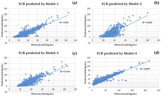
Figure 8.
Comparison of RMSEs of (a) Model 1, (b) Model 2, (c) Model 3 and (d) Model 4.
Although Model 3 showed the highest improvement in predictive performance, with an increase of 19.72% compared to Model 1, Model 4, and Model 2, which had increases of 18.42%, 17.41%, and 7.19%, respectively, it is not considered the best model in this study due to its significantly higher RMSE compared to the other models. Therefore, it is not recommended to use this model for making real predictions.
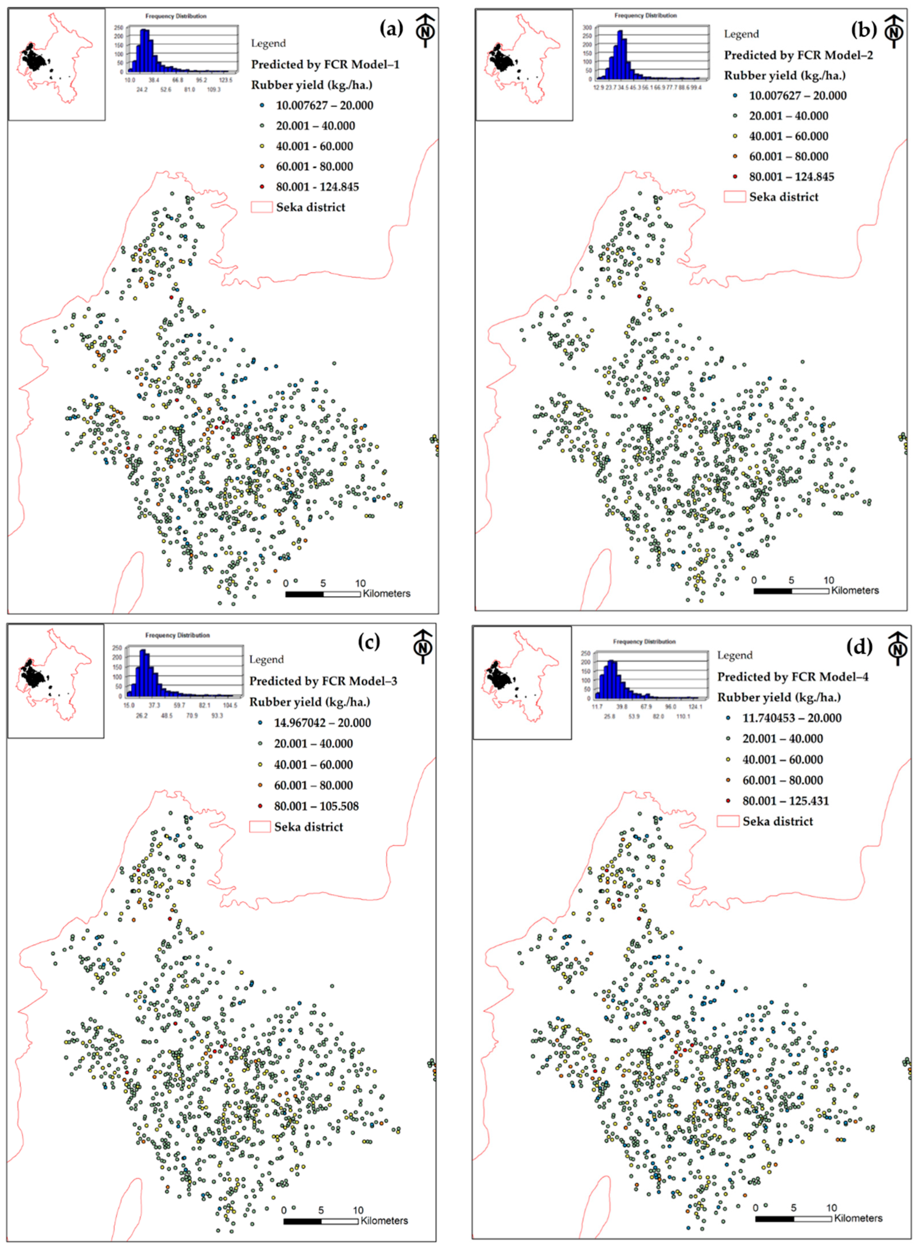
The prediction results are displayed using point-based spatial data, which represent the central locations of 1104 rubber plots shown in Figure 9a−d. This is due to the lower tolerance of the two models compared to the others. However, it is worth noting that, despite this, the maximum yield values predicted by Models 1 and 4 are similar. This is because the location and dispersion of the yield plots are both low. These predictions will be used to determine where the model should be applied next.
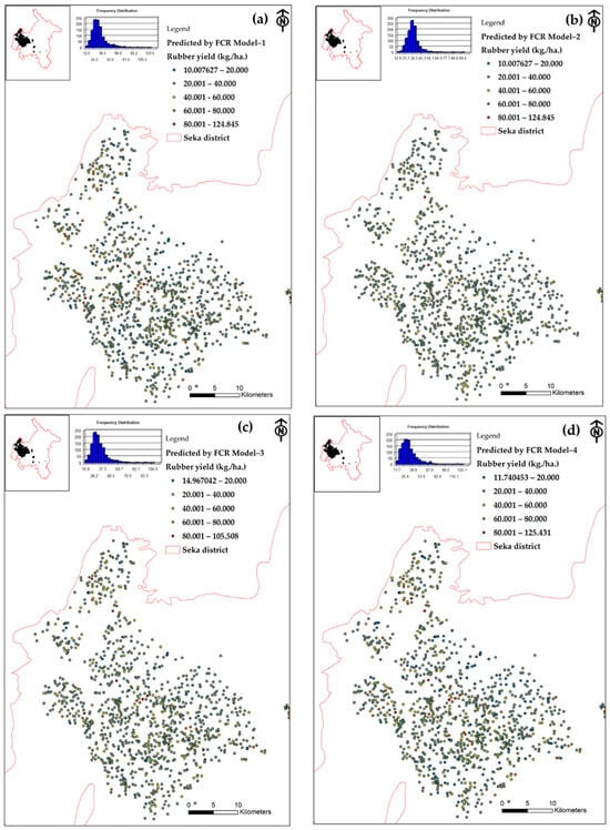
Figure 9.
The mappings of rubber yields predicted by (a) Model 1, (b) Model 2, (c) Model 3 and (d) Model 4.
4. Discussion
4.1. Focusing on the Areas Where the Projected Rubber Yield Results Were Implemented
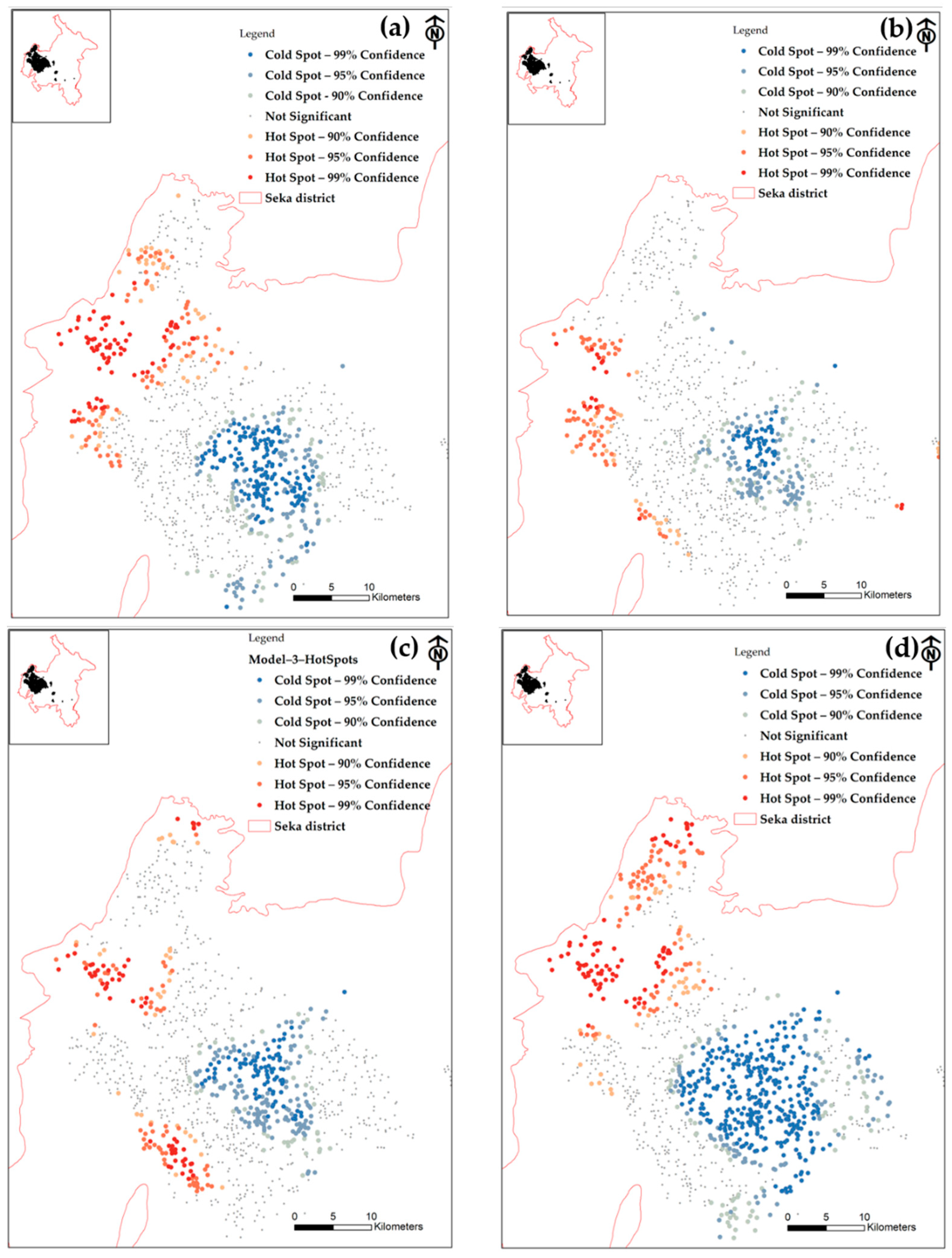
To better understand the Getis–Ord Gi* results for cold spots at 90, 95, and 99% confidence levels, it is important to grasp that these values indicate the certainty that a particular spatial location is indeed a cold spot, meaning an area with lower-than-expected values. When a cold spot has a 90% confidence level, this means that there is a 90% probability that the observed values in that location are lower than what would be expected by chance alone. This suggests a relatively high degree of certainty that the location is indeed a cold spot. A cold spot with a 95% confidence level indicates an even higher level of confidence that the observed values are lower than would be expected by chance. This implies a greater level of certainty compared to the 90% confidence level. Finally, a cold spot with a 99% confidence level represents the highest level of certainty, as depicted in Figure 10.
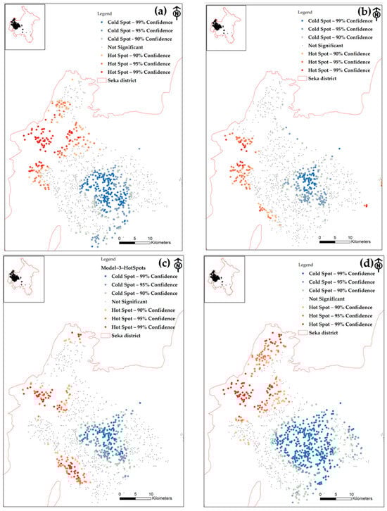
Figure 10.
The results of the hot-spot analysis (Getis–Ord Gi*) for four models: (a) Model 1, (b) Model 2, (c) Model 3, and (d) Model 4.
4.2. Model Validation
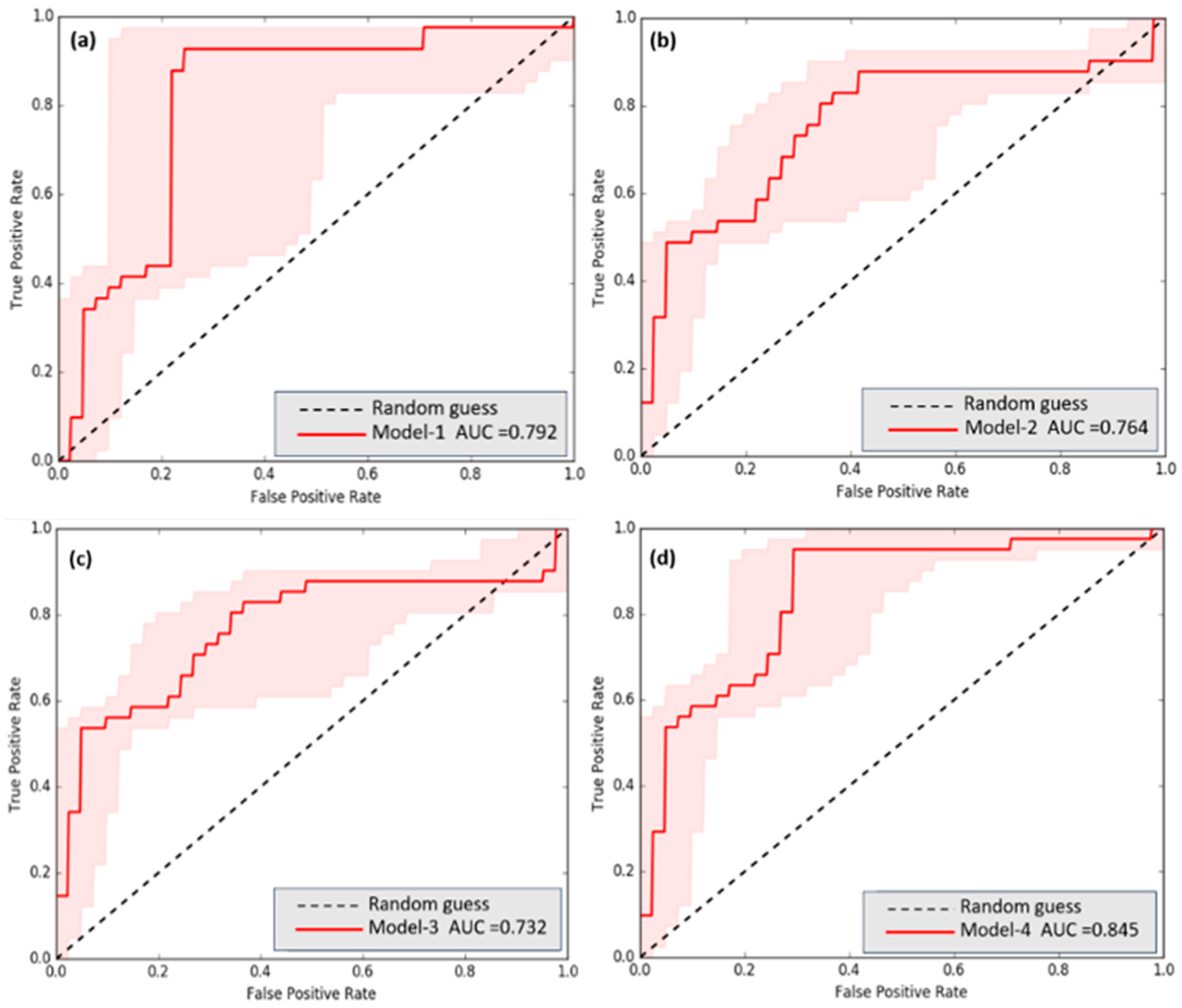
The positions used to compare the correct predictions in terms of position in the calibration of this model were derived from the hot spots analyzed through the hot-spot analysis (Getis–Ord Gi*). Only the hot spots that the model predicted and which did not exceed the RMSE value of each model were considered. This assumed that the yield points of the plots were accurately predicted. The results from the four models indicate that Model 4 achieved the highest AUC score of 0.845. Following this, Model 1 obtained an AUC score of 0.792, Model 2 scored 0.764, and Model 3 scored 0.732. Overall, Model 4 demonstrated the best classification performance based on the AUC scores. Conversely, Model 3 performed the poorest, as it obtained the lowest AUC score. It is worth noting that while AUC is commonly used to evaluate binary classification models, it is advisable to consider other performance metrics, such as accuracy, precision, recall, and F1-score, for a more comprehensive evaluation of a model’s performance, as depicted in Figure 11.
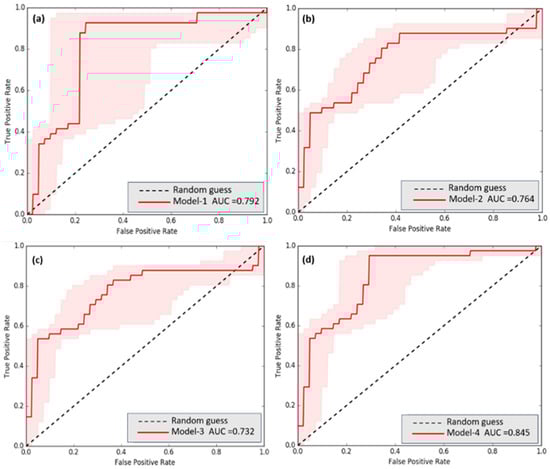
Figure 11.
The FCR alternative models’ area under the curves (AUCs): (a) Model 1, (b) Model 2, (c) Model 3, and (d) Model 4.
4.3. Comparison of the Results Obtained with Previous Work
Most of the previous research in the field predominantly relied on linear and non-linear modeling, as well as machine learning methods, to forecast rubber yields. The findings consistently indicate that the RF method offers more precise predictions compared to other methods, with AUC values of 0.8 or higher. However, the accuracy of the predictions is contingent upon the quality of the set of independent variables employed for forecasting. Previously, there were limitations in the application of independent variables across various regions, resulting in significant disparities in the results. To address this issue, our study focuses on assessing rubber yield predictions in areas conducive to yield enhancement, taking into account the specific rubber varieties, fertilizer usage, soil characteristics, and the local climate. Essentially, our study introduces a new set of independent variables to discern the prediction outcomes based on different groups of rubber yields. The classification of these groups based on independent variables has been recalibrated to suit areas with a high concentration of rubber plantations. These variables can effectively determine the expected yield in regions characterized by varying independent-variable values. Notably, this novel research approach has not been previously attempted, allowing our results to show a distinct contrast to the adoption of distinct sets of independent variables.
To promote consistency in sustainable development goals (SDGs), it is important to apply the results of the analysis of influence factors to the studied area. These factors include the distance from the river, slope, and aspect. By controlling the size of the rubber plantation area and still achieving a high yield per area, we can ensure a balance between the two. The amount of rainfall is an uncontrollable factor that affects latex production. These factors indicate the amount of latex produced based on the model’s results. Therefore, in areas where sustainable spatial development is desired to prevent environmental impacts caused by rubber plantation expansion, it is recommended to focus on increasing production per unit area in locations that have suitable levels of these factors. This approach will allow for the design of areas that can maximize production.
5. Conclusions
The development of FCR machine learning in the high-density area of rubber fields is based on simulation and divided into four sub-models. This serves as an alternative method for predicting the yield of lump rubber. In every test conducted, the model was found to be more accurate than the original model. The incorporation of a distinct set of independent variables to distinguish the region can enhance the effectiveness of the FCR model in accurately projecting the actual rubber yield. This improvement is reflected in the AUC ranging between 0.732 and 0.845 and an error margin in the rubber yield forecast of 15.87 to 30.26 kg per hectare. These results indicate a satisfactory level of predictive accuracy. Interested individuals can download the zip files, labeled as Supplementary Materials, which contain the geographic information system (GIS) data for the study area. These files include the necessary independent variable data and can be utilized for conducting preliminary modeling experiments.
This study can serve as a blueprint for forecasting rubber yields, ensuring that the integrity of the planting area is at an appropriate level. Furthermore, the study proposes the inclusion of spatial factors that could potentially enhance yield by considering soil surface moisture levels throughout the production season. Consequently, this approach could be applied in areas near rivers in other countries to predict rubber yields with an acceptable level of accuracy. In future studies, several machine learning models could be compared to determine the most efficient method for forecasting.
Supplementary Materials
The following supporting information can be downloaded at: https://www.mdpi.com/article/10.3390/f15091535/s1.
Author Contributions
Conceptualization, P.L., W.K., B.P. and W.K.; methodology, P.L. and B.P.; testing, N.P., S.S. and N.B.; writing—original draft preparation, P.L.; writing—review and editing, P.L. and D.S.; supervision, P.L.; project administration P.L. All authors have read and agreed to the published version of the manuscript.
Funding
This research project was financially supported by Mahasarakham University in 2025 (number: 2-2568) for spatial analysis and GIS laboratory usage. This work was supported by the Rubber Authority of Thailand (RAOT) 2024 (number: 020-2567).
Data Availability Statement
The original data presented in the study are openly available and can be downloaded as Supplement Files.
Conflicts of Interest
The authors declare no conflicts of interest.
References
- Bhumiphan, N.; Nontapon, J.; Kaewplang, S.; Srihanu, N.; Koedsin, W.; Huete, A. Estimation of Rubber Yield Using Sentinel-2 Satellite Data. Sustainability 2023, 15, 7223. [Google Scholar] [CrossRef]
- Yasen, K.; Koedsin, W. Estimating Aboveground Biomass of Rubber Tree Using Remote Sensing in Phuket Province, Thailand. J. Med. Bioeng. 2015, 4, 451–456. [Google Scholar] [CrossRef]
- Rao, P.S.; Saraswathyamma, C.K.; Sethuraj, M.R. Studies on the Relationship between Yield and Meteorological Parameters of Para Rubber Tree (Hevea Brasiliensis). Agric. For. Meteorol. 1998, 90, 235–245. [Google Scholar] [CrossRef]
- Krukanont, P.; Prasertsan, S. Geographical Distribution of Biomass and Potential Sites of Rubber Wood Fired Power Plants in Southern Thailand. Biomass Bioenergy 2004, 26, 47–59. [Google Scholar] [CrossRef]
- Chantuma, P.; Lacote, R.; Leconte, A.; Gohet, E. An Innovative Tapping System, the Double Cut Alternative, to Improve the Yield of Hevea Brasiliensis in Thai Rubber Plantations. Field Crops Res. 2011, 121, 416–422. [Google Scholar] [CrossRef]
- Nath, A.J.; Brahma, B.; Kumar Das, A. No TitleRubber Plantations and Carbon Management, 1st ed.; Apple Academic Press: Palm Bay, FL, USA, 2019; p. 166. [Google Scholar] [CrossRef]
- Liu, X.; Feng, Z.; Jiang, L.; Li, P.; Liao, C.; Yang, Y.; You, Z. Rubber Plantation and Its Relationship with Topographical Factors in the Border Region of China, Laos and Myanmar. J. Geogr. Sci. 2013, 23, 1019–1040. [Google Scholar] [CrossRef]
- Dauwalter, D.C.; Fesenmyer, K.A.; Bjork, R.; Leasure, D.R.; Wenger, S.J. Satellite and Airborne Remote Sensing Applications for Freshwater Fisheries. Fisheries 2017, 42, 526–537. [Google Scholar] [CrossRef]
- Gao, S.; Liu, X.; Bo, Y.; Shi, Z.; Zhou, H. Rubber Identification Based on Blended High Spatio-Temporal Resolution Optical Remote Sensing Data: A Case Study in Xishuangbanna. Remote Sens. 2019, 11, 496. [Google Scholar] [CrossRef]
- Nguyen, M.D.; Baez–Villanueva, O.M.; Bui, D.D.; Nguyen, P.T.; Ribbe, L. Harmonization of Landsat and Sentinel 2 for Crop Monitoring in Drought Prone Areas: Case Studies of Ninh Thuan (Vietnam) and Bekaa (Lebanon). Remote Sens. 2020, 12, 281. [Google Scholar] [CrossRef]
- Songsaengrit, S.; Kangrang, A. Dynamic Rule Curves and Streamflow under Climate Change for Multipurpose Reservoir Operation Using Honey–Bee Mating Optimization. Sustainability 2022, 14, 8599. [Google Scholar] [CrossRef]
- Zhang, M.; Lin, H.; Wang, G.; Sun, H.; Fu, J. Mapping Paddy Rice Using a Convolutional Neural Network (CNN) with Landsat 8 Datasets in the Dongting Lake Area, China. Remote Sens. 2018, 10, 1840. [Google Scholar] [CrossRef]
- Rao, D.V.K.N.; Jose, A.I.; Rao, A.V.R.K. Spectral Signature and Temporal Variation in Spectral Reflectance: Keys to Identify Rubber Vegetation. In Proceedings of the International Symposium on Remote Sensing, Crete, Greece, 17 March 2003; Volume 4879, pp. 114–124. [Google Scholar]
- Li, Z.; Fox, J.M. Mapping Rubber Tree Growth in Mainland Southeast Asia Using Time–Series MODIS 250 m NDVI and Statistical Data. Appl. Geogr. 2012, 32, 420–432. [Google Scholar] [CrossRef]
- Zhiming, F.; Luguang, J.; Xiaona, L.I.U.; Jinghua, Z. Rubber Plantations in Xishuangbanna: Remote Sensing Identification and Digital Mapping. Resour. Sci. 2012, 34, 1769–1780. [Google Scholar]
- Fan, H.; Fu, X.; Zhang, Z.; Wu, Q. Phenology-Based Vegetation Index Differencing for Mapping of Rubber Plantations Using Landsat OLI Data. Remote Sens. 2015, 7, 6041–6058. [Google Scholar] [CrossRef]
- Somching, N.; Wongsai, S.; Wongsai, N.; Koedsin, W. Using Machine Learning Algorithm and Landsat Time Series to Identify Establishment Year of Para Rubber Plantations: A Case Study in Thalang District, Phuket Island, Thailand. Int. J. Remote Sens. 2020, 41, 9075–9100. [Google Scholar] [CrossRef]
- Reynolds, C.A.; Yitayew, M.; Slack, D.C.; Hutchinson, C.F.; Huete, A.; Petersen, M.S. Estimating Crop Yields and Production by Integrating the FAO Crop Specific Water Balance Model with Real-Time Satellite Data and Ground-Based Ancillary Data. Int. J. Remote Sens. 2000, 21, 3487–3508. [Google Scholar] [CrossRef]
- Azizan, F.A.; Kiloes, A.M.; Astuti, I.S.; Aziz, A.A. Application of Optical Remote Sensing in Rubber Plantations: A Systematic Review. Remote Sens. 2021, 13, 429. [Google Scholar] [CrossRef]
- Whitcraft, A.K.; Becker-Reshef, I.; Justice, C.O.; Gifford, L.; Kavvada, A.; Jarvis, I. No Pixel Left behind: Toward Integrating Earth Observations for Agriculture into the United Nations Sustainable Development Goals Framework. Remote Sens. Environ. 2019, 235, 111470. [Google Scholar] [CrossRef]
- Bastiaanssen, W.G.M.; Ali, S. A New Crop Yield Forecasting Model Based on Satellite Measurements Applied across the Indus Basin, Pakistan. Agric. Ecosyst. Environ. 2003, 94, 321–340. [Google Scholar] [CrossRef]
- Rodriguez, J.C.; Duchemin, B.; Hadria, R.; Watts, C.; Garatuza, J.; Chehbouni, A.; Khabba, S.; Boulet, G.; Palacios, E.; Lahrouni, A. Wheat Yield Estimation Using Remote Sensing and the STICS Model in the Semiarid Yaqui Valley, Mexico. Agronomie 2004, 24, 295–304. [Google Scholar] [CrossRef]
- Chandra Paul, G.; Saha, S.; Hembram, T.K. Application of Phenology–Based Algorithm and Linear Regression Model for Estimating Rice Cultivated Areas and Yield Using Remote Sensing Data in Bansloi River Basin, Eastern India. Remote Sens. Appl. Soc. Environ. 2020, 19, 100367. [Google Scholar] [CrossRef]
- Zhang, P.-P.; Zhou, X.-X.; Wang, Z.-X.; Mao, W.; Li, W.-X.; Yun, F.; Guo, W.-S.; Tan, C.-W. Using HJ-CCD Image and PLS Algorithm to Estimate the Yield of Field-Grown Winter Wheat. Sci. Rep. 2020, 10, 5173. [Google Scholar] [CrossRef]
- Al–Gaadi, K.A.; Hassaballa, A.A.; Tola, E.; Kayad, A.G.; Madugundu, R.; Alblewi, B.; Assiri, F. Prediction of Potato Crop Yield Using Precision Agriculture Techniques. PLoS ONE 2016, 11, e0162219. [Google Scholar] [CrossRef]
- Awad, M.M. Toward Precision in Crop Yield Estimation Using Remote Sensing and Optimization Techniques. Agriculture 2019, 9, 54. [Google Scholar] [CrossRef]
- Gómez, D.; Salvador, P.; Sanz, J.; Casanova, J.L. Potato yield prediction using machine learning techniques and sentinel 2 data. Remote Sens. 2019, 11, 1745. [Google Scholar] [CrossRef]
- Goel, P.K.; Prasher, S.O.; Patel, R.M.; Landry, J.A.; Bonnell, R.B.; Viau, A.A. Classification of Hyperspectral Data by Decision Trees and Artificial Neural Networks to Identify Weed Stress and Nitrogen Status of Corn. Comput. Electron. Agric. 2003, 39, 67–93. [Google Scholar] [CrossRef]
- Ferencz, C.; Bognár, P.; Lichtenberger, J.; Hamar, D.; Tarcsai†, G.; Timár, G.; Molnár, G.; Pásztor, S.Z.; Steinbach, P.; Székely, B.; et al. Crop Yield Estimation by Satellite Remote Sensing. Int. J. Remote Sens. 2004, 25, 4113–4149. [Google Scholar] [CrossRef]
- Uno, Y.; Prasher, S.O.; Lacroix, R.; Goel, P.K.; Karimi, Y.; Viau, A.; Patel, R.M. Artificial Neural Networks to Predict Corn Yield from Compact Airborne Spectrographic Imager Data. Comput. Electron. Agric. 2005, 47, 149–161. [Google Scholar] [CrossRef]
- Peng, Y.; Gitelson, A.A. Application of Chlorophyll–Related Vegetation Indices for Remote Estimation of Maize Productivity. Agric. For. Meteorol. 2011, 151, 1267–1276. [Google Scholar] [CrossRef]
- Maresma, Á.; Lloveras, J.; Martínez-Casasnovas, J.A. Use of Multispectral Airborne Images to Improve In–Season Nitrogen Management, Predict Grain Yield and Estimate Economic Return of Maize in Irrigated High Yielding Environments. Remote Sens. 2018, 10, 543. [Google Scholar] [CrossRef]
- Van Kraalingen, D.W.G.; Breure, C.J.; Spitters, C.J.T. Simulation of Oil Palm Growth and Yield. Agric. For. Meteorol. 1989, 46, 227–244. [Google Scholar] [CrossRef]
- Chong, K.L.; Kanniah, K.D.; Pohl, C.; Tan, K.P. A Review of Remote Sensing Applications for Oil Palm Studies. Geo-Spat. Inf. Sci. 2017, 20, 184–200. [Google Scholar] [CrossRef]
- Hashemvand Khiabani, P.; Takeuchi, W. Assessment of Oil Palm Yield and Biophysical Suitability in Indonesia and Malaysia. Int. J. Remote Sens. 2020, 41, 8520–8546. [Google Scholar] [CrossRef]
- Rashid, M.; Bari, B.S.; Yusup, Y.; Kamaruddin, M.A.; Khan, N. A Comprehensive Review of Crop Yield Prediction Using Machine Learning Approaches With Special Emphasis on Palm Oil Yield Prediction. IEEE Access 2021, 9, 63406–63439. [Google Scholar] [CrossRef]
- Chang, K.-W.; Shen, Y.; Lo, J.-C. Predicting Rice Yield Using Canopy Reflectance Measured at Booting Stage. Agron. J. 2005, 97, 872–878. [Google Scholar] [CrossRef]
- Cui, B.; Huang, W.; Ye, H.; Chen, Q. The Suitability of PlanetScope Imagery for Mapping Rubber Plantations. Remote Sens. 2022, 14, 1061. [Google Scholar] [CrossRef]
- Dong, J.; Xiao, X.; Chen, B.; Torbick, N.; Jin, C.; Zhang, G.; Biradar, C. Mapping Deciduous Rubber Plantations through Integration of PALSAR and Multi–Temporal Landsat Imagery. Remote Sens. Environ. 2013, 134, 392–402. [Google Scholar] [CrossRef]
- Li, P.; Zhang, J.; Feng, Z. Mapping Rubber Tree Plantations Using a Landsat–Based Phenological Algorithm in Xishuangbanna, Southwest China. Remote Sens. Lett. 2015, 6, 49–58. [Google Scholar] [CrossRef]
- Xiao, C.; Li, P.; Feng, Z.; Liu, X. An Updated Delineation of Stand Ages of Deciduous Rubber Plantations during 1987–2018 Using Landsat-Derived Bi-Temporal Thresholds Method in an Anti-Chronological Strategy. Int. J. Appl. Earth Obs. Geoinf. 2019, 76, 40–50. [Google Scholar] [CrossRef]
- Li, J.; Roy, D.P. A Global Analysis of Sentinel-2A, Sentinel-2B and Landsat-8 Data Revisit Intervals and Implications for Terrestrial Monitoring. Remote Sens. 2017, 9, 902. [Google Scholar] [CrossRef]
- Singh, D.; Slik, J.W.F.; Jeon, Y.S.; Tomlinson, K.W.; Yang, X.; Wang, J.; Kerfahi, D.; Porazinska, D.L.; Adams, J.M. Tropical Forest Conversion to Rubber Plantation Affects Soil Micro– & Mesofaunal Community & Diversity. Sci. Rep. 2019, 9, 5893. [Google Scholar] [CrossRef]
- Ullah, T.; Muhammad, Z.; Shah, I.A.; Bourhia, M.; Nafidi, H.A.; Salamatullah, A.M.; Younous, Y.A. Multivariate Analysis of the Summer Herbaceous Vegetation and Environmental Factors of the Sub-Tropical Region. Sci. Rep. 2024, 14, 15657. [Google Scholar] [CrossRef] [PubMed]
- Hazir, M.H.M.; Muda, T.M.T. The Viability of Remote Sensing for Extracting Rubber Smallholding Information: A Case Study in Malaysia. Egypt. J. Remote Sens. Space Sci. 2020, 23, 35–47. [Google Scholar] [CrossRef]
- Littidej, P.; Buasri, N. Built–up Growth Impacts on Digital Elevation Model and Flood Risk Susceptibility Prediction in Muaeng District, Nakhon Ratchasima (Thailand). Water 2019, 11, 1496. [Google Scholar] [CrossRef]
- Littidej, P.; Uttha, T.; Pumhirunroj, B. Spatial Predictive Modeling of the Burning of Sugarcane Plots in Northeast Thailand with Selection of Factor Sets Using a GWR Model and Machine Learning Based on an ANN-CA. Symmetry 2022, 14, 1989. [Google Scholar] [CrossRef]
- Pumhirunroj, B.; Littidej, P.; Boonmars, T.; Bootyothee, K.; Artchayasawat, A.; Khamphilung, P.; Slack, D. Machine-Learning-Based Forest Classification and Regression (FCR) for Spatial Prediction of Liver Fluke Opisthorchis Viverrini (OV) Infection in Small Sub-Watersheds. ISPRS Int. J. Geo-Inf. 2023, 12, 503. [Google Scholar] [CrossRef]
- Prasertsri, N.; Littidej, P. Spatial Environmental Modeling for Wildfire Progression Accelerating Extent Analysis Using Geo-Informatics. Pol. J. Environ. Stud. 2020, 29, 3249–3261. [Google Scholar] [CrossRef]
- Hussain, M.A.; Chen, Z.; Zheng, Y.; Shoaib, M.; Shah, S.U.; Ali, N.; Afzal, Z. Landslide Susceptibility Mapping Using Machine Learning Algorithm Validated by Persistent Scatterer In–SAR Technique. Sensors 2022, 22, 3119. [Google Scholar] [CrossRef]
- Achour, Y.; Pourghasemi, H.R. How Do Machine Learning Techniques Help in Increasing Accuracy of Landslide Susceptibility Maps? Geosci. Front. 2020, 11, 871–883. [Google Scholar] [CrossRef]
- Kumar, R.; Anbalagan, R. Landslide Susceptibility Mapping Using Analytical Hierarchy Process (AHP) in Tehri Reservoir Rim Region, Uttarakhand. J. Geol. Soc. India 2016, 87, 271–286. [Google Scholar] [CrossRef]
- Tengtrairat, N.; Woo, W.L.; Parathai, P.; Aryupong, C.; Jitsangiam, P.; Rinchumphu, D. Automated Landslide-Risk Prediction Using Web GIS and Machine Learning Models. Sensors 2021, 21, 4620. [Google Scholar] [CrossRef]
- Park, S.; Choi, C.; Kim, B.; Kim, J. Landslide Susceptibility Mapping Using Frequency Ratio, Analytic Hierarchy Process, Logistic Regression, and Artificial Neural Network Methods at the Inje Area, Korea. Environ. Earth Sci. 2013, 68, 1443–1464. [Google Scholar] [CrossRef]
- Tien Bui, D.; Pradhan, B.; Lofman, O.; Revhaug, I. Landslide Susceptibility Assessment in Vietnam Using Support Vector Machines, Decision Tree, and Naïve Bayes Models. Math. Probl. Eng. 2012, 2012, 974638. [Google Scholar] [CrossRef]
- Mandal, S.; Mandal, K. Modeling and Mapping Landslide Susceptibility Zones Using GIS Based Multivariate Binary Logistic Regression (LR) Model in the Rorachu River Basin of Eastern Sikkim Himalaya, India. Model. Earth Syst. Environ. 2018, 4, 69–88. [Google Scholar] [CrossRef]
- Pourghasemi, H.R.; Rahmati, O. Prediction of the Landslide Susceptibility: Which Algorithm, Which Precision? Catena 2018, 162, 177–192. [Google Scholar] [CrossRef]
- Youssef, A.M.; Pourghasemi, H.R.; Pourtaghi, Z.S.; Al-Katheeri, M.M. Landslide Susceptibility Mapping Using Random Forest, Boosted Regression Tree, Classification and Regression Tree, and General Linear Models and Comparison of Their Performance at Wadi Tayyah Basin, Asir Region, Saudi Arabia. Landslides 2016, 13, 839–856. [Google Scholar] [CrossRef]
- Rossi, M.; Guzzetti, F.; Reichenbach, P.; Mondini, A.C.; Peruccacci, S. Optimal Landslide Susceptibility Zonation Based on Multiple Forecasts. Geomorphology 2010, 114, 129–142. [Google Scholar] [CrossRef]
- Park, S.; Kim, J. Landslide Susceptibility Mapping Based on Random Forest and Boosted Regression Tree Models, and a Comparison of Their Performance. Appl. Sci. 2019, 9, 942. [Google Scholar] [CrossRef]
- Sevgen, E.; Kocaman, S.; Nefeslioglu, H.A.; Gokceoglu, C. A Novel Performance Assessment Approach Using Photogrammetric Techniques for Landslide Susceptibility Mapping with Logistic Regression, ANN and Random Forest. Sensors 2019, 19, 3940. [Google Scholar] [CrossRef]
- Pérez-Díaz, P.; Martín-Dorta, N.; Gutiérrez-García, F.J. Construction Labour Measurement in Reinforced Concrete Floating Caissons in Maritime Ports. Civ. Eng. J. 2022, 8, 195–208. [Google Scholar] [CrossRef]
- Hussain, M.A.; Chen, Z.; Wang, R.; Shoaib, M. PS-InSAR-Based Validated Landslide Susceptibility Mapping along Karakorum Highway, Pakistan. Remote Sens. 2021, 13, 4129. [Google Scholar] [CrossRef]
- Taalab, K.; Cheng, T.; Zhang, Y. Mapping Landslide Susceptibility and Types Using Random Forest. Big Earth Data 2018, 2, 159–178. [Google Scholar] [CrossRef]
- Conoscenti, C.; Ciaccio, M.; Caraballo-Arias, N.A.; Gómez-Gutiérrez, Á.; Rotigliano, E.; Agnesi, V. Assessment of Susceptibility to Earth–Flow Landslide Using Logistic Regression and Multivariate Adaptive Regression Splines: A Case of the Belice River Basin (Western Sicily, Italy). Geomorphology 2015, 242, 49–64. [Google Scholar] [CrossRef]
- Felicísimo, Á.M.; Cuartero, A.; Remondo, J.; Quirós, E. Mapping Landslide Susceptibility with Logistic Regression, Multiple Adaptive Regression Splines, Classification and Regression Trees, and Maximum Entropy Methods: A Comparative Study. Landslides 2013, 10, 175–189. [Google Scholar] [CrossRef]
- Vorpahl, P.; Elsenbeer, H.; Märker, M.; Schröder, B. How Can Statistical Models Help to Determine Driving Factors of Landslides? Ecol. Model. 2012, 239, 27–39. [Google Scholar] [CrossRef]
- Ghasemian, B.; Shahabi, H.; Shirzadi, A.; Al-Ansari, N.; Jaafari, A.; Kress, V.R.; Geertsema, M.; Renoud, S.; Ahmad, A. A Robust Deep-Learning Model for Landslide Susceptibility Mapping: A Case Study of Kurdistan Province, Iran. Sensors 2022, 22, 1573. [Google Scholar] [CrossRef]
- Ma, J.; Wang, Y.; Niu, X.; Jiang, S.; Liu, Z. A Comparative Study of Mutual Information-Based Input Variable Selection Strategies for the Displacement Prediction of Seepage-Driven Landslides Using Optimized Support Vector Regression. Stoch. Environ. Res. Risk Assess. 2022, 36, 3109–3129. [Google Scholar] [CrossRef]
- Kalantar, B.; Pradhan, B.; Naghibi, S.A.; Motevalli, A.; Mansor, S. Assessment of the Effects of Training Data Selection on the Landslide Susceptibility Mapping: A Comparison between Support Vector Machine (SVM), Logistic Regression (LR) and Artificial Neural Networks (ANN). Geomat. Nat. Hazards Risk 2018, 9, 49–69. [Google Scholar] [CrossRef]
- Pham, B.T.; Tien Bui, D.; Pourghasemi, H.R.; Indra, P.; Dholakia, M.B. Landslide Susceptibility Assesssment in the Uttarakhand Area (India) Using GIS: A Comparison Study of Prediction Capability of Naïve Bayes, Multilayer Perceptron Neural Networks, and Functional Trees Methods. Theor. Appl. Climatol. 2017, 128, 255–273. [Google Scholar] [CrossRef]
- Pham, B.T.; Pradhan, B.; Tien Bui, D.; Prakash, I.; Dholakia, M.B. A Comparative Study of Different Machine Learning Methods for Landslide Susceptibility Assessment: A Case Study of Uttarakhand Area (India). Environ. Model. Softw. 2016, 84, 240–250. [Google Scholar] [CrossRef]
- Mehrabi, M.; Pradhan, B.; Moayedi, H.; Alamri, A. Optimizing an Adaptive Neuro-Fuzzy Inference System for Spatial Prediction of Landslide Susceptibility Using Four State-of-the-Art Metaheuristic Techniques. Sensors 2020, 20, 1723. [Google Scholar] [CrossRef] [PubMed]
- Dehnavi, A.; Aghdam, I.N.; Pradhan, B.; Morshed Varzandeh, M.H. A New Hybrid Model Using Step-Wise Weight Assessment Ratio Analysis (SWARA) Technique and Adaptive Neuro-Fuzzy Inference System (ANFIS) for Regional Landslide Hazard Assessment in Iran. Catena 2015, 135, 122–148. [Google Scholar] [CrossRef]
- Aghdam, I.N.; Varzandeh, M.H.M.; Pradhan, B. Landslide Susceptibility Mapping Using an Ensemble Statistical Index (Wi) and Adaptive Neuro–Fuzzy Inference System (ANFIS) Model at Alborz Mountains (Iran). Environ. Earth Sci. 2016, 75, 553. [Google Scholar] [CrossRef]
- Kumar, R.; Anbalagan, R. Landslide Susceptibility Zonation in Part of Tehri Reservoir Region Using Frequency Ratio, Fuzzy Logic and GIS. J. Earth Syst. Sci. 2015, 124, 431–448. [Google Scholar] [CrossRef]
- Charandabi, S.E.; Kamyar, K. Prediction of Cryptocurrency Price Index Using Artificial Neural Networks: A Survey of the Literature. Eur. J. Bus. Manag. Res. 2021, 6, 17–20. [Google Scholar] [CrossRef]
- Roshani, M.; Sattari, M.A.; Muhammad Ali, P.J.; Roshani, G.H.; Nazemi, B.; Corniani, E.; Nazemi, E. Application of GMDH Neural Network Technique to Improve Measuring Precision of a Simplified Photon Attenuation Based Two-Phase Flowmeter. Flow Meas. Instrum. 2020, 75, 101804. [Google Scholar] [CrossRef]
- Moayedi, H.; Osouli, A.; Tien Bui, D.; Foong, L.K. Spatial Landslide Susceptibility Assessment Based on Novel Neural-Metaheuristic Geographic Information System Based Ensembles. Sensors 2019, 19, 4698. [Google Scholar] [CrossRef]
- Bui, D.T.; Moayedi, H.; Kalantar, B.; Osouli, A.; Pradhan, B.; Nguyen, H.; Rashid, A.S. A Novel Swarm Intelligence—Harris Hawks Optimization for Spatial Assessment of Landslide Susceptibility. Sensors 2019, 19, 3590. [Google Scholar] [CrossRef]
- Arnone, E.; Francipane, A.; Scarbaci, A.; Puglisi, C.; Noto, L. V Effect of Raster Resolution and Polygon–Conversion Algorithm on Landslide Susceptibility Mapping. Environ. Model. Softw. 2016, 84, 467–481. [Google Scholar] [CrossRef]
- Aditian, A.; Kubota, T.; Shinohara, Y. Comparison of GIS-Based Landslide Susceptibility Models Using Frequency Ratio, Logistic Regression, and Artificial Neural Network in a Tertiary Region of Ambon, Indonesia. Geomorphology 2018, 318, 101–111. [Google Scholar] [CrossRef]
- Kornejady, A.; Ownegh, M.; Bahremand, A. Landslide Susceptibility Assessment Using Maximum Entropy Model with Two Different Data Sampling Methods. Catena 2017, 152, 144–162. [Google Scholar] [CrossRef]
- Park, N.-W. Using Maximum Entropy Modeling for Landslide Susceptibility Mapping with Multiple Geoenvironmental Data Sets. Environ. Earth Sci. 2015, 73, 937–949. [Google Scholar] [CrossRef]
- Dang, V.-H.; Hoang, N.-D.; Nguyen, L.-M.-D.; Bui, D.T.; Samui, P. A Novel GIS-Based Random Forest Machine Algorithm for the Spatial Prediction of Shallow Landslide Susceptibility. Forests 2020, 11, 118. [Google Scholar] [CrossRef]
- Wu, X.; Ren, F.; Niu, R. Landslide Susceptibility Assessment Using Object Mapping Units, Decision Tree, and Support Vector Machine Models in the Three Gorges of China. Environ. Earth Sci. 2014, 71, 4725–4738. [Google Scholar] [CrossRef]
- Merghadi, A.; Yunus, A.P.; Dou, J.; Whiteley, J.; ThaiPham, B.; Bui, D.T.; Avtar, R.; Abderrahmane, B. Machine Learning Methods for Landslide Susceptibility Studies: A Comparative Overview of Algorithm Performance. Earth-Sci. Rev. 2020, 207, 103225. [Google Scholar] [CrossRef]
- Sahin, E.K. Comparative Analysis of Gradient Boosting Algorithms for Landslide Susceptibility Mapping. Geocarto Int. 2022, 37, 2441–2465. [Google Scholar] [CrossRef]
- Pumhirunroj, B.; Littidej, P.; Boonmars, T.; Artchayasawat, A.; Prasertsri, N.; Khamphilung, P.; Sangpradid, S.; Buasri, N.; Uttha, T.; Slack, D. Spatial Predictive Modeling of Liver Fluke Opisthorchis Viverrine (OV) Infection under the Mathematical Models in Hexagonal Symmetrical Shapes Using Machine Learning–Based Forest Classification Regression. Symmetry 2024, 16, 1067. [Google Scholar] [CrossRef]
- Guo, P.-T.; Zhu, A.-X.; Cha, Z.-Z.; Li, M.-F.; Luo, W. A Local Model Based on Environmental Variables Clustering for Estimating Foliar Phosphorus of Rubber Trees with Vis–NIR Spectroscopic Data. Heliyon 2022, 8, e09795. [Google Scholar] [CrossRef]
- Bunmi Mudashiru, R.; Sabtu, N.; Abdullah, R.; Saleh, A.; Abustan, I. Optimality of Flood Influencing Factors for Flood Hazard Mapping: An Evaluation of Two Multi-Criteria Decision-Making Methods. J. Hydrol. 2022, 612, 128055. [Google Scholar] [CrossRef]
- Breiman, L. Random Forests. Mach. Learn. 2001, 45, 5–32. [Google Scholar] [CrossRef]
- Cutler, A.; Cutler, D.R.; Stevens, J.R. Random Forests BT–Ensemble Machine Learning: Methods and Applications; Zhang, C., Ma, Y., Eds.; Springer: New York, NY, USA, 2012; pp. 157–175. ISBN 978-1-4419-9326-7. [Google Scholar]
- Belgiu, M.; Drăguţ, L. Random Forest in Remote Sensing: A Review of Applications and Future Directions. ISPRS J. Photogramm. Remote Sens. 2016, 114, 24–31. [Google Scholar] [CrossRef]
- Li, H.; Beldring, S.; Xu, C.-Y.; Huss, M.; Melvold, K.; Jain, S.K. Integrating a Glacier Retreat Model into a Hydrological Model–Case Studies of Three Glacierised Catchments in Norway and Himalayan Region. J. Hydrol. 2015, 527, 656–667. [Google Scholar] [CrossRef]
- Prinzie, A.; Van den Poel, D. Random Multiclass Classification: Generalizing Random Forests to Random MNL and Random NB BT–Database and Expert Systems Applications; Wagner, R., Revell, N., Pernul, G., Eds.; Springer: Berlin/Heidelberg, Germany, 2007; pp. 349–358. [Google Scholar]
- Choubin, B.; Borji, M.; Mosavi, A.; Sajedi–Hosseini, F.; Singh, V.P.; Shamshirband, S. Snow Avalanche Hazard Prediction Using Machine Learning Methods. J. Hydrol. 2019, 577, 123929. [Google Scholar] [CrossRef]
- Wang, H.; Zheng, H. True Positive Rate BT–Encyclopedia of Systems Biology; Dubitzky, W., Wolkenhauer, O., Cho, K.-H., Yokota, H., Eds.; Springer: New York, NY, USA, 2013; pp. 2302–2303. ISBN 978-1-4419-9863-7. [Google Scholar]
- Fawcett, T. An Introduction to ROC Analysis. Pattern Recognit. Lett. 2006, 27, 861–874. [Google Scholar] [CrossRef]
- Fan, J.; Upadhye, S.; Worster, A. Understanding Receiver Operating Characteristic (ROC) Curves. Can. J. Emerg. Med. 2006, 8, 19–20. [Google Scholar] [CrossRef]

Disclaimer/Publisher’s Note: The statements, opinions and data contained in all publications are solely those of the individual author(s) and contributor(s) and not of MDPI and/or the editor(s). MDPI and/or the editor(s) disclaim responsibility for any injury to people or property resulting from any ideas, methods, instructions or products referred to in the content. |
© 2024 by the authors. Licensee MDPI, Basel, Switzerland. This article is an open access article distributed under the terms and conditions of the Creative Commons Attribution (CC BY) license (https://creativecommons.org/licenses/by/4.0/).