Abstract
The Henan Yellow River Basin is an ecological support belt for the entire basin. It holds a significant position in high-quality development and ecological conservation within the Yellow River Basin. However, due to improper development activities, such as urban expansion and deforestation of farmland, certain areas of the region have encountered a series of ecological issues, posing significant challenges to ecosystem services. The scientific foundation for the sustainable development of the ecological environment in the Henan Yellow River Basin is established by research on the evolution characteristics and driving factors of ecosystem service functions. This study focuses on the Henan Yellow River Basin, by introducing remote sensing data and biomass data, assessing the spatiotemporal variations in ecosystem service by the InVEST model—including carbon stock, water yield, and soil conservation—from 2000 to 2020. It analyzes the ecosystem service functions of different land use types. It employs the Geodetector to identify the dominant driving factors behind the changes in these functions based on the improved InVEST model evaluated results. The findings reveal that from 2000 to 2020, total carbon stock increased by 1.86%, carbon stock per unit area rose by 1.81%, and the spatial distribution remained largely stable. The high-value regions were clustered in the west and part of the north, primarily consisting of forest land. Carbon stock capacity in other regions, mainly farmland and construction land, was poor, with forest land having the strongest carbon sequestration capacity, followed by grassland. Total water yield decreased by 20.08%, and water yield per unit area decreased by 20.03%, with a spatial distribution closely following the trend of precipitation distribution. The high-value regions were clustered in the south, primarily in forest land and farmland. The total amount of soil conservation decreased by 19.96%, and soil conservation per unit area decreased by 19.93%, with spatial distribution patterns similar to those of carbon stock and water yield. The high-value regions were concentrated in the southwestern and northern forested regions, while soil conservation capacity in areas primarily consisting of farmland and construction land was weaker. The divergence of carbon stock was most influenced by population density, water yield by precipitation, and soil conservation by slope. In conclusion, during the study period, while carbon storage increased, the significant decline in water yield and soil conservation highlighted critical issues in the ecosystem service functions of the region. These findings indicate the need for targeted conservation measures and sustainable development strategies to address the decline in ecosystem services and mitigate adverse environmental impacts, ensuring the long-term health of the region’s ecosystems. This study offers an in-depth understanding of the differentiation of ecosystem service functions and their driving factors, enabling precise assessment of regional ecosystem services, and providing a theoretical foundation for formulating effective regional ecological conservation policies.
1. Introduction
Ecosystem services refer to products and services necessary for survival obtained directly or indirectly through the ecosystem’s structure, processes, and functions. They form and maintain the conditions and utilities of the natural environment [1,2,3,4]. Ecosystems provide raw materials and products essential for human survival and perform functions like wind and sand control, hydrological regulation, nutrient cycling, and soil formation, known as ecosystem service functions [5,6]. These services are characterized by distinct spatial and temporal patterns, influenced by a variety of natural and social driving factors. Understanding the evolution of these services over time provides a scientific foundation for the formulation of sustainable development and ecological preservation policies, which is of significant practical importance for achieving global ecological civilization [7,8].
The comprehensive evaluation of ecosystem service functions has become a significant concern for researchers and scholars globally. As early as the mid-19th century, George Marsh first recorded ecosystem service functions in “Man and Nature” [9]. The concept of “ecosystem service function” was clarified by Holdren and Ehrlich in the 1970s [10]. In 2013, Huang et al. provided an overview of 10 ecosystem service function assessment models [11]. Among these, the InVEST model is the most broadly utilized for evaluating ecosystem service functions, with numerous studies conducted both domestically and internationally [12,13,14,15,16,17]. However, when assessing ecosystem service functions, the InVEST model sometimes simplifies and assumes certain complex ecosystem processes, affecting the exactness of the results [18]. Additionally, the choice and setting of different parameters in the model can lead to significant differences in the assessment outcomes, for example, the carbon stock module [19,20]. The selection of an appropriate carbon estimation method therefore requires further research.
The ecosystem services in China exhibit complexity and diversity due to rapid economic development, urbanization, and distinctive environmental challenges [21]. Urban expansion and agricultural intensification have led to dramatic changes in land use patterns, exerting substantial pressure on key ecosystem services, including water resource regulation, soil conservation, and carbon storage [22]. To improve the ecological environment, reduce ecological pressure, and promote the sustainable development of the socio-economy, a series of ecological protection policies have been implemented in China, since 1998, including the Grain for Green Project and the Natural Forest Protection Project [23,24]. As China’s second-longest and the world’s fifth-longest river [25], the Yellow River provides ecosystem services that are crucial for ecological security and significantly impact regional and global ecosystems [26]. Its research has made a major issue within the world of academia [27,28,29,30]. The Henan Yellow River Basin spans its middle and lower reaches, serving as a significant ecological transition belt connecting the Loess Plateau and the Yellow and Huaihai Plains, and bearing significant responsibility for maintaining regional ecological security [31]. As a major population center, grain production base, and energy hub in China, the study area has been subjected to irrational development activities such as mineral resource exploitation, inefficient water use, and agricultural over-fertilization, which urgently need enhanced capacity to provide ecological products [32,33,34]. Since 2000, the aforementioned ecological protection policies have been fully implemented in the Henan Yellow River Basin, following national directives. By 2010, the first phase of China’s Natural Forest Conservation Project had been completed, with the second phase reaching completion by 2020 [35]. The Grain for Green Project, initiated in 2002, continues to the present [36]. The actual effects of these policies, along with their impact on regional ecosystem services, need long-term assessment to optimize policy design and implementation.
Taking the Henan Yellow River Basin as the study area, assessing the ecosystem service functions of this area, clarifies the spatiotemporal evolution of these functions, and employs the Geodetector to analyze the dominant driving factors influencing changes in ecosystem services. It is hypothesized that the spatiotemporal characteristics in ecosystem services in the study area from 2000 to 2020 have undergone certain changes and are primarily driven by variations in topography, climate change, and socio-economic developments. The aim is to propose ecosystem management strategies for the Henan Yellow River Basin, providing insights for sustainable resource use and conservation, and supporting the region’s sustainable development and ecological protection.
2. Materials and Methods
2.1. Overview of the Study Area
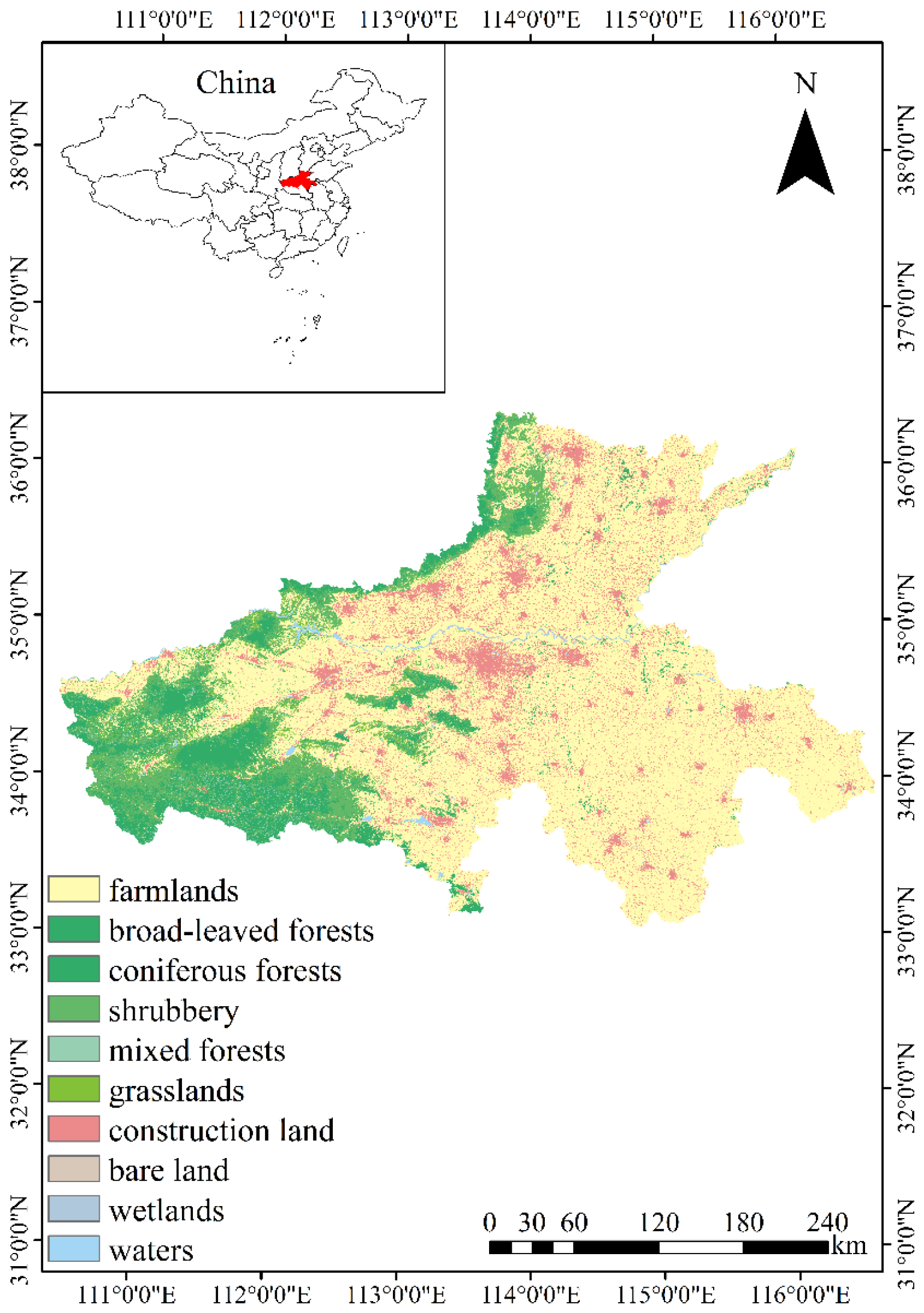
The Henan Yellow River Basin (111° E–117° E, 33° N–36° N) is located in the middle and lower reaches of the Yellow River Basin, extending through eight provincial municipalities with a total length of 711 km. Grounded in its natural geographic characteristics, the Yellow River Basin consists of the core area, the expansion area, and the Yellow Diversion Collaboration Area. The watershed, the area along the Yellow River, and the Yellow River Diversion Receiving Area encompass a total of 120 counties (cities and districts) in 14 provincial municipalities, covering an overall area of about 102,500 km2 (Figure 1). The study area spans the central, western, eastern, and northern parts of Henan Province, featuring a varied terrain with elevations ranging from 26.58 to 1101.67 m.

Figure 1.
The study area and its geographic location.
The research area is situated within a continental monsoon climate zone, transitioning from the northern subtropical to the warm temperate zone. The region is primarily influenced by the atmospheric circulation of the westerly wind belt and exhibits a transition from plain to hilly and mountainous climates from east to west. It experiences distinct four seasons, concurrent rain and heat, a complex and diverse climate, and frequent climate-related disasters. The research area contains a diverse range of soil types: in the mountainous regions, the predominant soil types are deep brown soil, yellow-brown soil, and brown soil; the hilly areas are primarily characterized by yellow sandy soil, brown sandy soil, yellow-brown soil, and brown soil; while the plain areas mainly feature yellow soil, yellow-brown soil, yellow sandy soil, and tidal soil.
The main natural vegetation type in the research area is deciduous broad-leaved forest. However, due to significant differences in topography and environmental conditions, the vegetation distribution exhibits distinct horizontal and vertical zoning patterns. The western and northern regions possess high vegetation cover and rich biodiversity with numerous species, although the distribution is uneven. Some of the plains and hilly areas have experienced a significant decline in vegetation cover due to frequent human activities and the over-exploitation and utilization of land.
Economic activities in the research area are primarily based on agriculture, with grain production playing a crucial role in the province. Industrial development is relatively dispersed, with resource-based industries dominant. In 2000, the socio-economic conditions were underdeveloped, characterized by relatively low total and per capita GDP. Since 2000, total economic output has significantly increased due to the rapid development of the socio-economic system [37].
2.2. Data Sources
The data used in this study include remote sensing data, land cover data, meteorological data, soil data, and digital elevation model (DEM) data (Table 1).

Table 1.
Data sources.
Landsat image data are primarily utilized to estimate forest biomass. Given the extensive area of study, we account for issues such as cloud contamination in the data and ensure spatial and temporal comparability across different periods, Landsat reflectance products corrected for atmospheric and topographic effects in the GEE platform were used. Maximized synthetic NDVI and EVI data for the vegetation growing seasons were obtained for the years 2000, 2005, 2010, 2015, and 2020 in the study area.
The GEDI L4A data is a footprint-level product that provides biomass information for each laser footprint on the ground. Since most of the forests in the study area are deciduous, and to obtain high-quality forest biomass light patch data, GEDI L4A data products with dates between 1 May 2020, and 30 September 2020, were selected according to the climatic features of the study area.
MOD17A3, one of the MODIS data products, focuses on global net primary productivity (NPP) measurements and provides information on vegetation growth at a resolution of 500 m.
The land cover data were divided into ten land classes: farmland, broad-leaved forest, coniferous forest, shrubbery, coniferous and broad-leaved mixed, grassland, wetland, waters, bare land, and construction land.
Precipitation data generated through collation, computation, and spatial interpolation of daily observations from over 2000 meteorological stations across China, offers spatially interpolated annual precipitation data. Based on this dataset, the precipitation distribution map for the study area was extracted from the national map and resampled to ensure consistency with the resolution and projection coordinate system of the land use data. The annual average potential evapotranspiration data was similarly processed and resampled to match the resolution and projection coordinates of the land use data.
The maximum root depth in soil was produced with the same resolution, projection coordinate system, and data format as the land use data.
The DEM data were mosaicked and cropped to match the extent of the study area, resulting in an elevation map having a spatial resolution of 30 m. The reference ellipsoid employed was WGS84.
2.3. Functional Analysis of Ecosystem Services under the Invest Model
2.3.1. Carbon Stock Modules
The carbon stock module categorizes the ecosystem’s carbon stock into four primary carbon sinks: above-ground biomass carbon (Cabove), below-ground biomass carbon (Cbelow), soil carbon (Csoil), and dead organic carbon (Cdead) [38].
Following these principles, the carbon stock function of the Yellow River Basin in Henan was assessed for five periods from 2000 to 2020. The necessary data include a map of land use types and a table of the study area of the carbon sink (Table 2). The carbon sink data were derived from Jiang’s study on year-by-year land use and carbon stock changes in terrestrial ecosystems in the Central Plains Economic Zone [39].
Table 2.
InVEST model carbon stock module carbon sinks table (Unit: t/ha).
2.3.2. Water Yield Module
The water yield module operates on the water balance principle, calculating water yield using parameters including precipitation, soil depth, and potential evapotranspiration. The formula for the calculation is as follows:
where Yxj is the annual water yield of x in the jth ecosystem type. AETxj is the practical yearly evapotranspiration of x in the jth ecosystem type. Px is the annual precipitation of x. Rxj is the Budyko dryness index of x in the jth ecosystem type, given by the proportion of potential evapotranspiration to rainfall. represents the ratio between the plant’s available water content (AWCx) and annual rainfall, a parameter describing natural climatic soil properties as defined by Zhang et al. [40]. Z represents a seasonal factor that reflects seasonal precipitation distribution and depth, representing regional precipitation patterns and other hydrogeological features [40]. etox denotes the potential evapotranspiration of x. kxj is the vegetative ET coefficient, representing the proportion of evapotranspiration to potential evapotranspiration for x in the jth ecosystem type.
2.3.3. Soil Conservation Module
The assessment of soil conservation services in the InVEST model relies on the soil loss equation, which calculates the discrepancy between estimated and actual soil erosion. The formula is as follows:
where R represents the rainfall erosion factor; K represents the soil erosion factor; L represents the slope length factor; S represents the slope gradient factor; C represents the vegetation cover factor; and P is the factor for soil conservation measures.
2.4. Carbon Stock Estimation Based on Multi-Source Data
In the carbon module of the InVEST model, carbon stock is estimated solely based on the carbon density of various land use types, without considering differences in carbon sequestration capacity across ecosystems, thereby affecting the accuracy of the model’s estimations [19,20]. To enhance the accuracy of the evaluation, different biomass estimation methods were employed for various land use types to obtain carbon storage estimates.
For the inversion of forest biomass in the research area, the widely adopted remote sensing estimation method internationally was employed [41,42,43].
2.4.1. Feature Variable Extraction
Forest remote sensing features encompass spectral information, vegetation indices, and texture data [44]. Landsat reflectance products from the GEE platform, corrected for atmospheric and terrain effects, were utilized in this study. Cloud computing algorithms were applied to obtain high-quality NDVI and EVI-maximized synthetic data for the vegetation growth seasons of 2000, 2005, 2010, 2015, and 2020 in the study area. Biomass inversion was conducted using a combination of terrain parameters (Table 3) [41].
Table 3.
Forest aboveground biomass inversion parameters.
2.4.2. Forest Biomass Estimation Model
To select a suitable forest biomass estimation model, ArcGIS (Version 10.8, Redlands, CA, USA) was used to extract the feature information of its different features to the corresponding filtered tree forest light spot data. The test sample and training sample were randomly selected at a ratio of 3:7 to construct two models: random forest and geographically weighted regression. The evaluation indicators generated by the training of the test set were used to evaluate the models and to verify the estimation effect of different models on the biomass of tree forests in the study area (Table 4). R2 is the coefficient of determination, and RMSE is the root mean square error [44]. These two coefficients were selected as indicators for model accuracy validation, and the model with higher accuracy was chosen as the inversion model for this study.
Table 4.
Random forest and geographically weighted regression results for arbor forests.
Shrubbery ecosystems exhibit low spatial heterogeneity, with biomass corrected using Landsat NDVI data. Farmland and grassland ecosystems have even lower spatial heterogeneity, and their annual biomass corresponds to Net Primary Productivity (NPP). The estimation of biomass on non-forest land uses MOD17A3 NPP data, calculates the vegetation carbon storage in the study area based on 2.25% of biomass carbon occupied by dead organic matter carbon, root to stem ratio 6.23, and consistent carbon content recommended by the National Greenhouse Gas Inventory Guidelines [45,46].
Biomass carbon density is primarily subject to factors such as climate, topography, nitrogen deposition, hydrological conditions, and stand density, while soil carbon density is mostly affected by factors such as soil category, soil respiration flux, and vegetative coverage [47]. Table 5 shows the soil carbon density of different land use types. According to the literature, forest soil carbon stock density per unit area in Henan increases by 0.3 t/ha annually, which serves as the basis for adjusting the carbon density of forest soil [47]. Ultimately, the distribution of carbon stock in the study area, as well as total and per unit area carbon stock for different land types, were produced.
Table 5.
Soil carbon density for different land use types.
2.5. Geodetector-Based Analysis of Ecosystem Service Function Drivers
Geodetector is a statistical technique employed to detect spatial heterogeneity and identify drivers based on factors, interactions, risks, and ecological factors [48], which has advantages in quantitatively analyzing the driving mechanisms of ecosystem services [49,50,51].
The factor detector can determine to what extent the independent variable X accounts for the spatial heterogeneity in the dependent variable Y, expressed as follows [52]:
In the formula, h = 1, …, L represents the stratification (i.e., classification or partitioning) of variable Y or factor X. Nh and N denote the number of units in stratum h and the entire area. and are the variance of the Y values in stratum h and the entire area. SSW and SST indicate the sum of the intra-stratum variances and the total variance of the entire region. q has a value from 0 to 1, and the higher the value, the more pronounced the spatial heterogeneity of Y.
Following practical operational requirements, the drivers of ecosystem service functions selected in this study should be comprehensive. By referencing past experiences and extracting from similar driver systems, while also considering current conditions and available data, factors were ultimately chosen as the focus of this research in Table 6 [53,54,55,56,57,58]. Selecting population density and GDP as representatives of socio-economic factors can reflect other socio-economic factors, including land use policies, industrial activities, and agricultural practices, through various channels.
Table 6.
Driving factors of ecosystem service change in the study area.
3. Results and Analysis
3.1. InVEST Model Assessment Results and Analysis
3.1.1. Carbon Stock Assessment Analysis, 2000–2020
- (1)
- Spatial and temporal variations in carbon stock
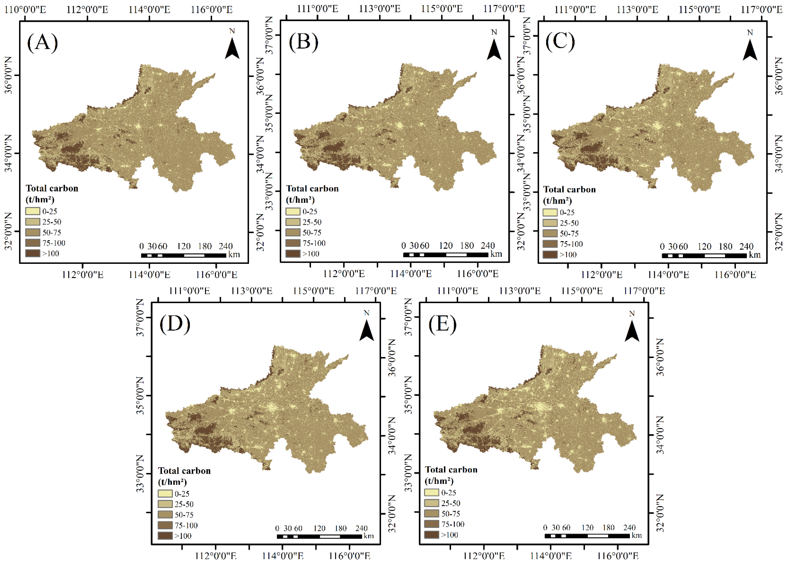
Figure 2 depicts carbon stock distribution in the study area across the period 2000–2020 under the InVEST. The spatial distribution of carbon stock during this period appears to have low spatial heterogeneity, which does not align with actual conditions. This discrepancy arises because the carbon stock module of the InVEST model focuses solely on the capability of carbon sequestration of various land use types, thereby compromising the accuracy of carbon stock estimates.
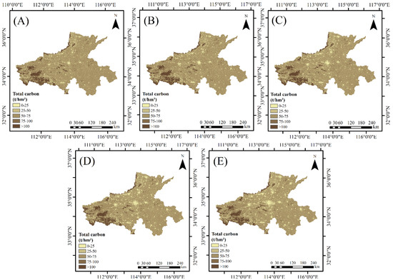
Figure 2.
Carbon stock distribution in the Yellow River Basin of Henan under the InVEST Model, 2000–2020 (unit: t/ha). (A) 2000; (B) 2005; (C) 2010; (D) 2015; (E) 2020.
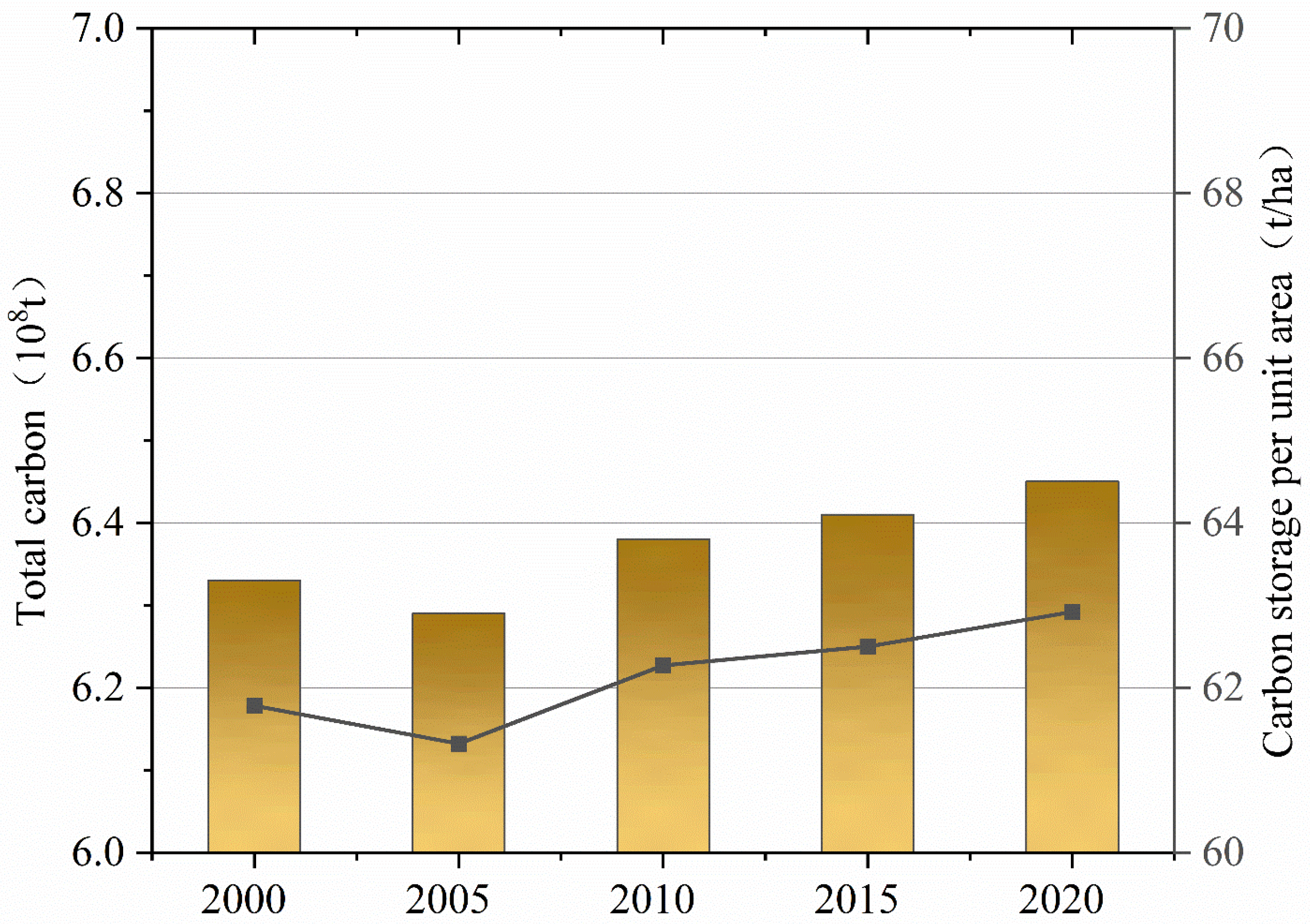
The results of the improved carbon stock assessment are shown in Figure 3. From 2000 to 2020, the total carbon stock increased from 6.33 × 10⁸ t to 6.45 × 10⁸ t, showing an overall upward trend. The carbon stock per unit area also rose from 61.78 t/ha in 2000 to 62.92 t/ha in 2020, indicating an increase rate of 1.81%. The most notable growth occurred from 2005 to 2010, with a rise of 9.74 × 10⁶ t, reflecting a growth rate of 1.55%. These findings suggest that while the overall trend in carbon stock remained stable, certain periods experienced more pronounced changes, likely driven by specific land use practices or environmental policies.

Figure 3.
Carbon stock changes in the study area, 2000–2020.
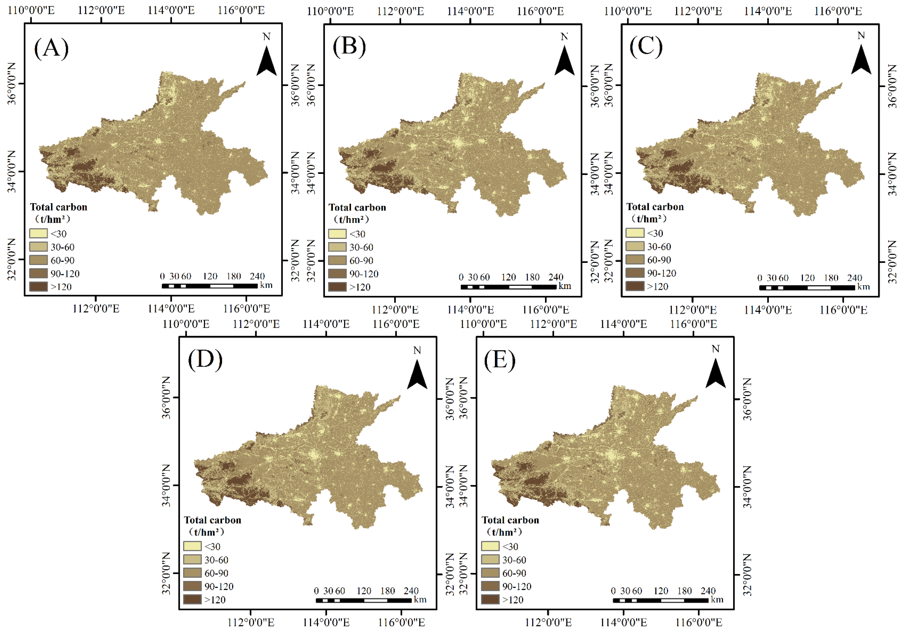
Spatially (Figure 4), higher carbon stock areas are concentrated in the western and northern regions, primarily characterized by forest land with dense vegetation and high coverage. The western mountainous areas, in particular, exhibit higher carbon sequestration potential due to better forest quality. In contrast, lower carbon stock is predominantly found in the eastern, southern, and central regions, where the primary land uses are farmland and construction areas, with less vegetation cover and higher surface hardening, leading to reduced carbon sequestration capacity. The results highlight the influence of land use and vegetation cover, with greater carbon sequestration potential observed in forested and mountainous areas, and diminished capacity in regions dominated by agriculture and urban development. This spatial variability underscores the critical role of topography and land use practices in driving changes in ecosystem services across the study area.
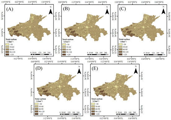
Figure 4.
Spatial distribution of Carbon Stock in the study area, 2000–2020. (A) 2000; (B) 2005; (C) 2010; (D) 2015; (E) 2020.
- (2)
- Carbon stock in different land types
The results (Table 7) indicate that, between 2000 and 2020, farmland consistently exhibited the highest carbon stock, comprising around 69% of the total carbon stock. It was followed by broadleaf forests and shrubbery, accounting for approximately 21% and 5.25% of the total carbon stock. In terms of carbon stock per unit area, broad-leaved forests ranked highest, followed by coniferous forests, mixed forests, and grasslands. Forest land exhibits the highest carbon sequestration capacity, and farmland holds the largest total carbon stock due to its extensive area. These findings suggest that carbon stock within the same land use type varies significantly due to extraneous factors for example climate conditions, soil conditions, vegetative type and cover, and human activities.
Table 7.
Results of carbon stock assessment for different land cover types.
3.1.2. Assessment and Analysis of Water Yield, 2000–2020
- (1)
- Spatial and temporal variations in water yield
The total water yield of the Henan Yellow River Basin from 2000 to 2020 exhibited a “declining–rising” trend (Figure 5). It decreased from 7.37 × 10¹⁰ m3 in 2000 to 5.23 × 10¹⁰ m3 in 2015, representing a reduction of 2.14 × 10¹⁰ m3, or 29.04%. Subsequently, water yield increased to 5.89 × 10¹⁰ m3 in 2020, marking a growth rate of 12.62%. The water yield per unit area followed the same trend as the total water production, decreasing by 1440 m3/ha. The results indicate that, despite a trend of recovery in recent years, overall water production significantly decreased during the entire study period. This trend is likely to have a critical impact on regional water resource management and planning.
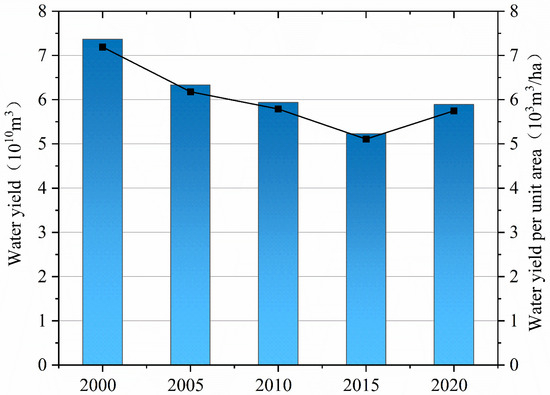
Figure 5.
Total water yield and water yield per unit area in the study area, 2000 to 2020.
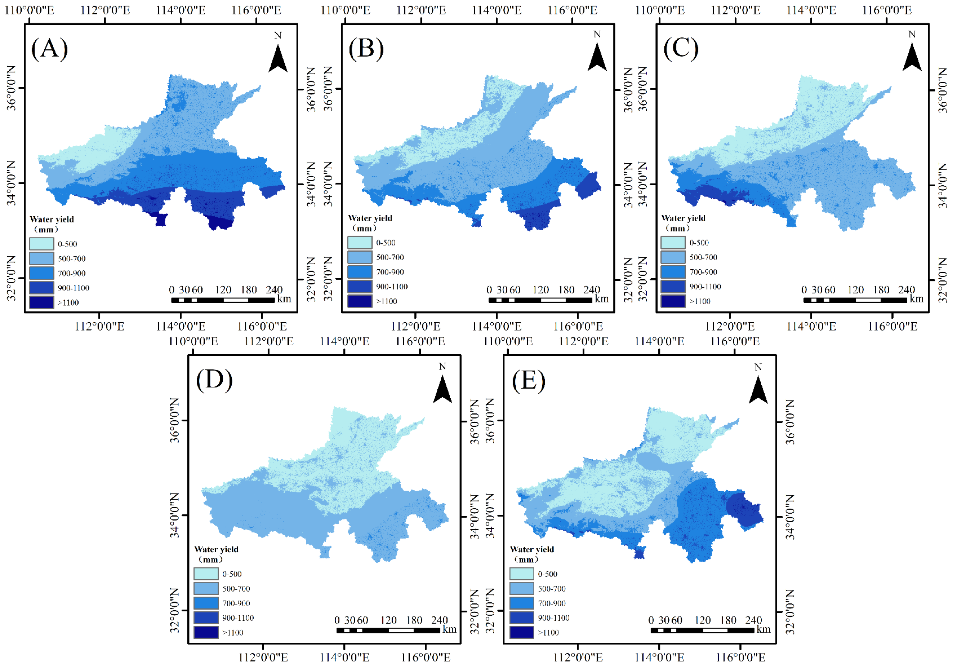
The spatial distribution of water yield from 2000 to 2020 (Figure 6) in the research area reveals a spatial trend with higher values in the southern regions and lower values in the northern, central, and western areas. The southern region predominantly features forested land and plain farmland, covered with vegetation that minimizes evaporation, favoring water retention. In contrast, areas with low water yield are primarily farmland and construction land, urban expansion and increased ground hardening due to population growth have diminished regional water retention capacity, resulting in lower water yields. Additionally, water yield is closely related to rainfall. As shown in Figure 7, the spatial distribution patterns of water yield are consistent with those of precipitation.
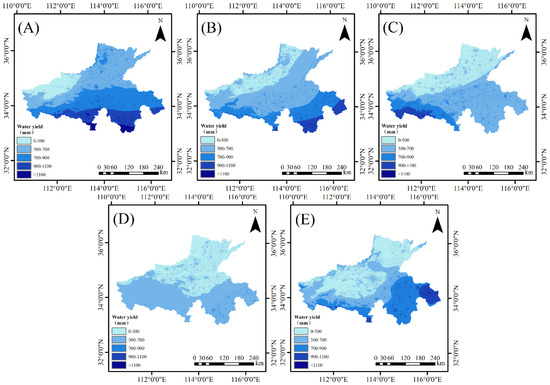
Figure 6.
Spatial distribution of water yield in the study area, 2000–2020. (A) 2000; (B) 2005; (C) 2010; (D) 2015; (E) 2020.
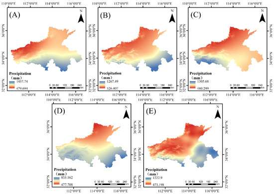
Figure 7.
Rainfall distribution of the study region. (A) 2000; (B) 2005; (C) 2010; (D) 2015; (E) 2020.
- (2)
- Water yield in different land use types
Table 8 presents the per unit area and total water yield of diverse land use types in the Henan Yellow River Basin. The results indicate that the water yield density of diverse land types, from highest to lowest, is as follows: coniferous and broad-leaved mixed, construction land, broad-leaved forests, coniferous forests, shrubbery, bare land, grassland, agricultural land, waters, and wetlands, and the total water yield from highest to lowest is farmland, broad-leaved forest, construction land, shrubbery, grassland, coniferous forest, coniferous and broad-leaved mixed, watershed, wetland, and bare land.
Table 8.
Results of water yield assessment for diverse land use types.
The study area is situated in the north-central part of the country, characterized by insufficient rainfall. Consequently, although the evapotranspiration of forested land is higher, the water-holding ability of other land types is much lower, thereby giving forested land a stronger water-holding capacity. The Henan Yellow River Basin is dominated by agriculture, with farmland comprising 70% of the total region, consistently contributing the largest total water yield, averaging 63.34% of the basin’s total water yield from 2000 to 2020. The dominance of agriculture in the basin underscores the significant role of farmland in the overall water yield.
3.1.3. Soil Conservation Assessment Analysis from 2000 to 2020
- (1)
- Spatiotemporal changes in soil conservation
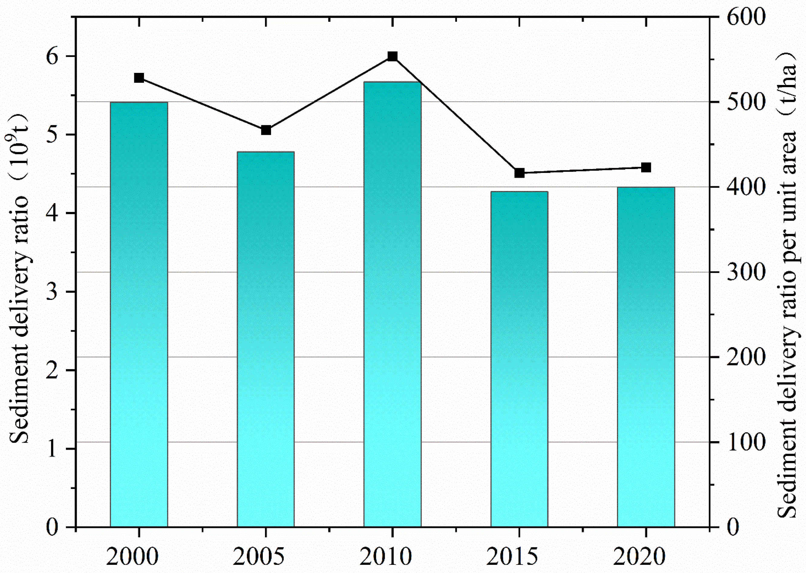
The assessment results (Figure 8) indicated that soil conservation in the study area exhibited significant fluctuations from 2000 to 2020, with an overall decreasing trend. Total soil conservation decreased from 5.41 × 10⁹ t in 2000 to 4.33 × 10⁹ t in 2020, representing a net reduction of 1.08 × 10⁹ t. The trend was characterized by periods of decline and recovery, with soil conservation peaking in 2010 at 5.67 × 10⁹ t and reaching its lowest point in 2015 at 4.27 × 10⁹ t. Soil conservation per unit area mirrored the overall trend, decreasing from 528.08 t/ha in 2000 to 422.85 t/ha in 2020. The most significant decline occurred between 2010 and 2015, with a reduction of 24.78%, while the smallest change was observed from 2015 to 2020, with a slight increase of 1.58%.

Figure 8.
Total soil conservation and soil conservation per unit area in the study area, 2000–2020.
The fluctuations are likely driven by variations in topography, climate change, and socio-economic developments, as hypothesized. The overall downward trend in soil conservation emphasizes the need for targeted interventions to improve soil retention in the region.
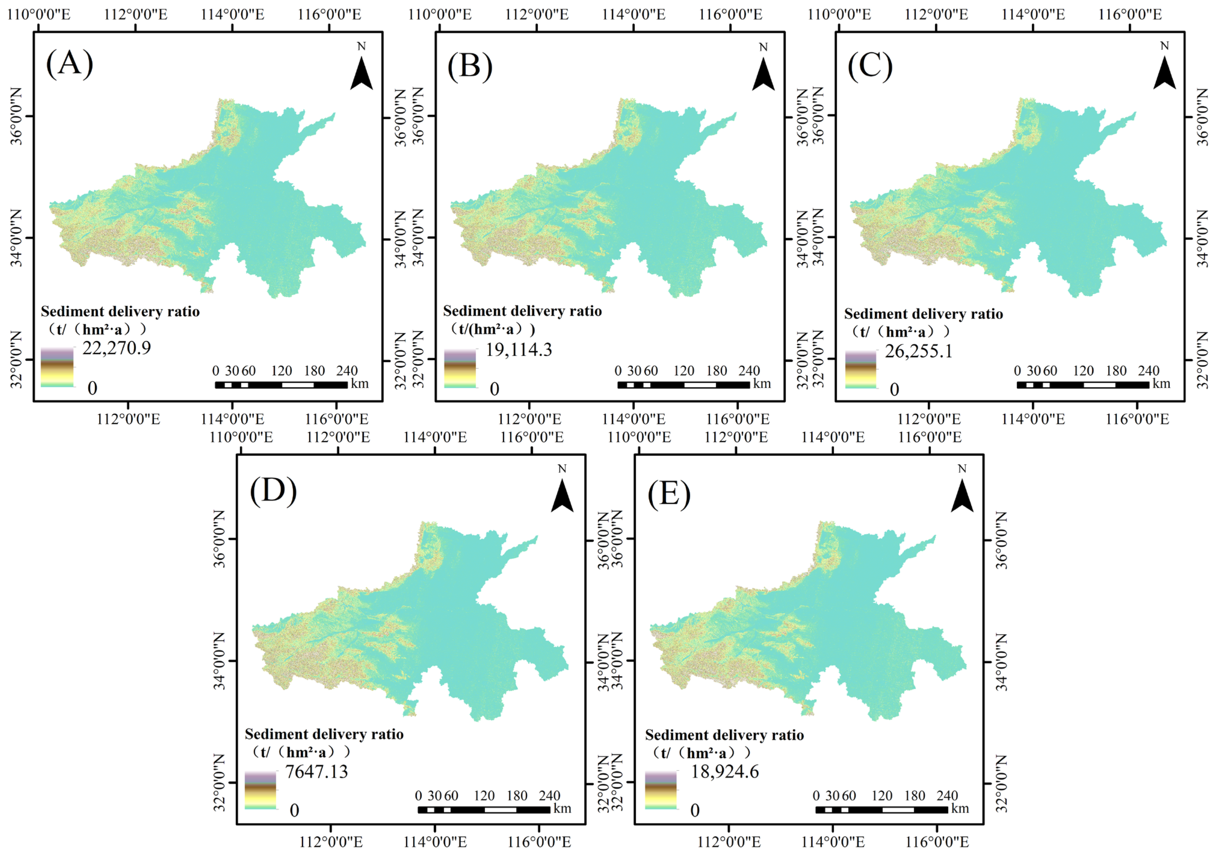
Regarding spatial characteristics (Figure 9), areas with higher soil conservation are primarily clustered in the southwestern and a small part of the northern area, where the main land cover type is dominated by forested land, resulting in higher soil conservation levels. In contrast, soil conservation in the eastern, southeastern, and central regions of the study area is lower. These regions mainly consist of farmland and construction land, which, along with factors such as rainfall erosion and soil erosion, lead to relatively low soil conservation functions.
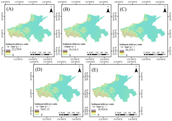
Figure 9.
Soil conservation’s spatial distribution in the study area, 2000–2020. (A) 2000; (B) 2005; (C) 2010; (D) 2015; (E) 2020.
The findings suggest that the southwestern and northern forested regions within the study area consistently exhibited higher soil conservation, whereas the agricultural and urbanized regions in the east, southeast, and center encountered difficulties in soil conservation.
- (2)
- Soil conservation in diverse land types
In Table 9, the total soil conservation result indicates that forest land consistently accounts for the largest percentage of soil conservation from 2000 to 2020, with an average of 80.66%. Farmland follows, averaging 14.76%. Grassland, construction land, water, wetland, and bare land follow in descending order. Compared to other land categories, bare land, wetland, and water cover less area and possess a weaker soil conservation effect. The analysis indicates that forest land plays a predominant role in soil conservation within the Henan Yellow River Basin, significantly exceeding the contributions of other land types. This underscores the critical importance of high biodiversity and dense vegetation cover in enhancing soil conservation.
Table 9.
Soil conservation assessment results for diverse land use types.
3.2. Analysis of Drivers of Ecosystem Service Function
3.2.1. Analysis of Carbon Stock Drivers
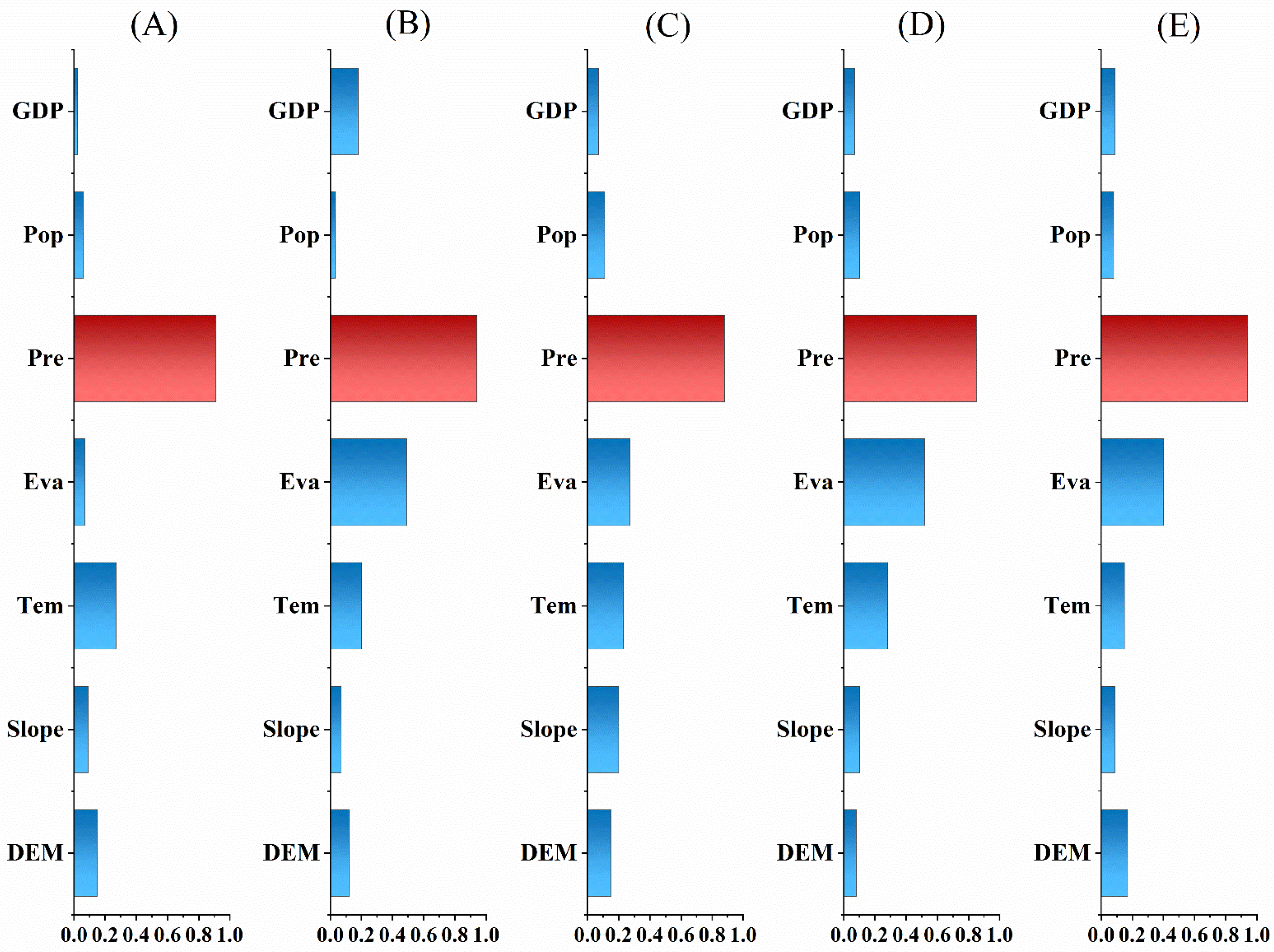
The drivers from 2000 to 2020, in descending order of the multi-year average q-value, are (Figure 10): population density (0.755) > GDP (0.644) > elevation (0.397) > slope (0.347) > mean annual temperature (0.313) > mean annual precipitation (0.162) > mean annual evapotranspiration (0.079). The results indicate that population density, GDP, elevation, slope, and temperature have a strong influence, with population density having the strongest power of explaining, making it the dominant driver of carbon stock changes.
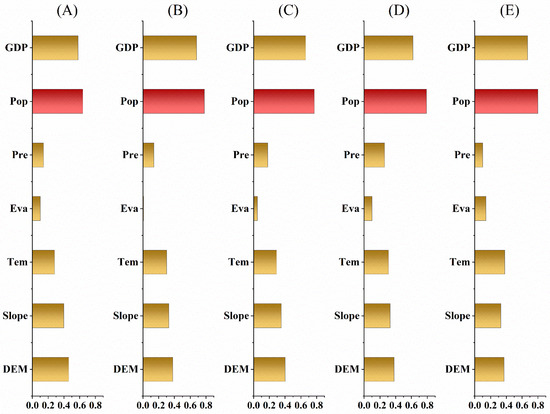
Figure 10.
Q-value of driving factors for carbon stock in the study area, 2000–2020. (A) 2000; (B) 2005; (C) 2010; (D) 2015; (E) 2020. Red: Indicates the highest q-value for the driving factor.
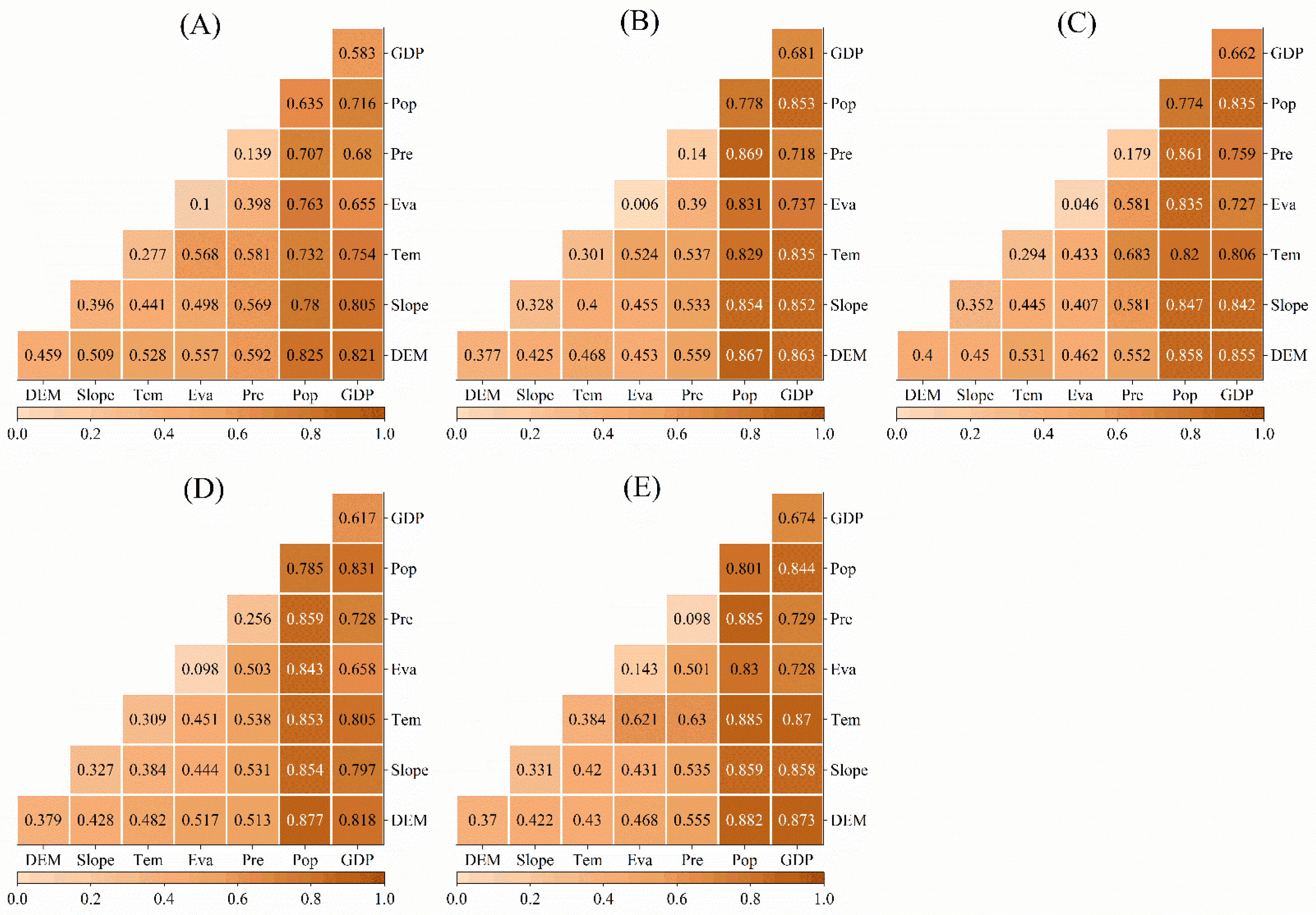
The results, shown in Figure 11, indicate that in the study of the drivers of carbon stock changes in the study area between 2000 and 2020, the interactions between the two factors are greater than that of a single factor. The most significant interaction occurred between elevation (DEM) and population density, with an explanatory power exceeding 0.707 and 0.831 in 2000 and 2015, respectively. This is consistent with the strongest explanatory power of population factors on carbon stock changes in single-factor analysis. In 2005, 2010, and 2020, the interaction between rainfall and population density exhibited the strongest influence on changes in carbon storage, with explanatory powers exceeding 0.829, 0.820, and 0.830, respectively. The interaction between population density and other factors consistently exhibited high explanatory power.
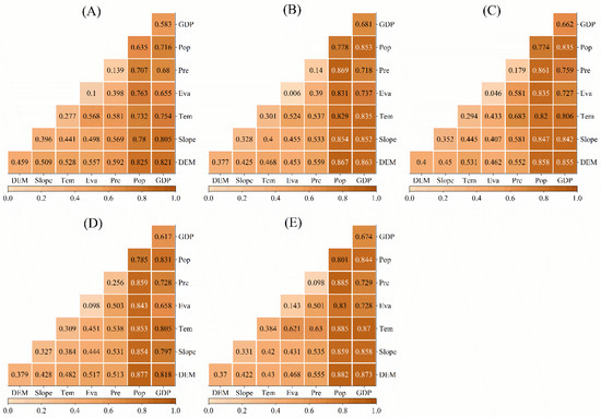
Figure 11.
Detection of two-factor interactions affecting carbon stock changes in the study area. (A) 2000; (B) 2005; (C) 2010; (D) 2015; (E) 2020.
The findings confirm that changes in carbon stock within the study area are primarily influenced by the interactions between population density and natural factors, including elevation and rainfall. Consequently, future development strategies should prioritize environmental protection and focus interventions on areas with low carbon stock to achieve a more balanced distribution and enhance overall carbon storage across the region.
3.2.2. Analysis of Water Yield Drivers
As shown in Figure 12, mean annual precipitation is the leading factor affecting water yield variation. The q values for mean annual precipitation were 0.906, 0.941, 0.883, 0.853, and 0.937 from 2000 to 2020, which was the most significant factor among the seven analyzed. The next significant factors were mean annual evapotranspiration and average annual temperature, with mean influence values of 0.352 and 0.226 over the past 20 years. Elevation and slope also influenced water yield, with mean q values of 0.134 and 0.110 over the past 20 years, respectively. In summary, mean annual precipitation, evapotranspiration, and temperature are the major factors influencing the distribution of water yield.
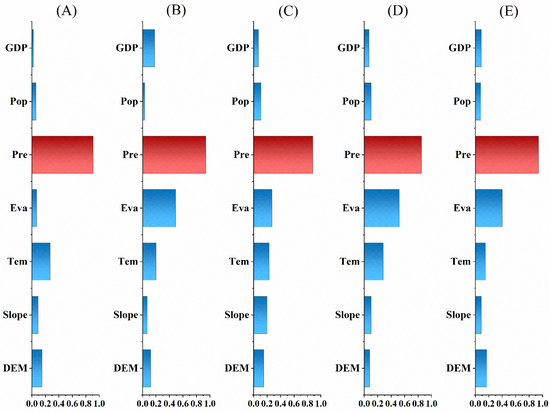
Figure 12.
Q-value of driving factors for water yield in the study area, 2000–2020. (A) 2000; (B) 2005; (C) 2010; (D) 2015; (E) 2020. Red: Indicates the highest q-value for the driving factor.
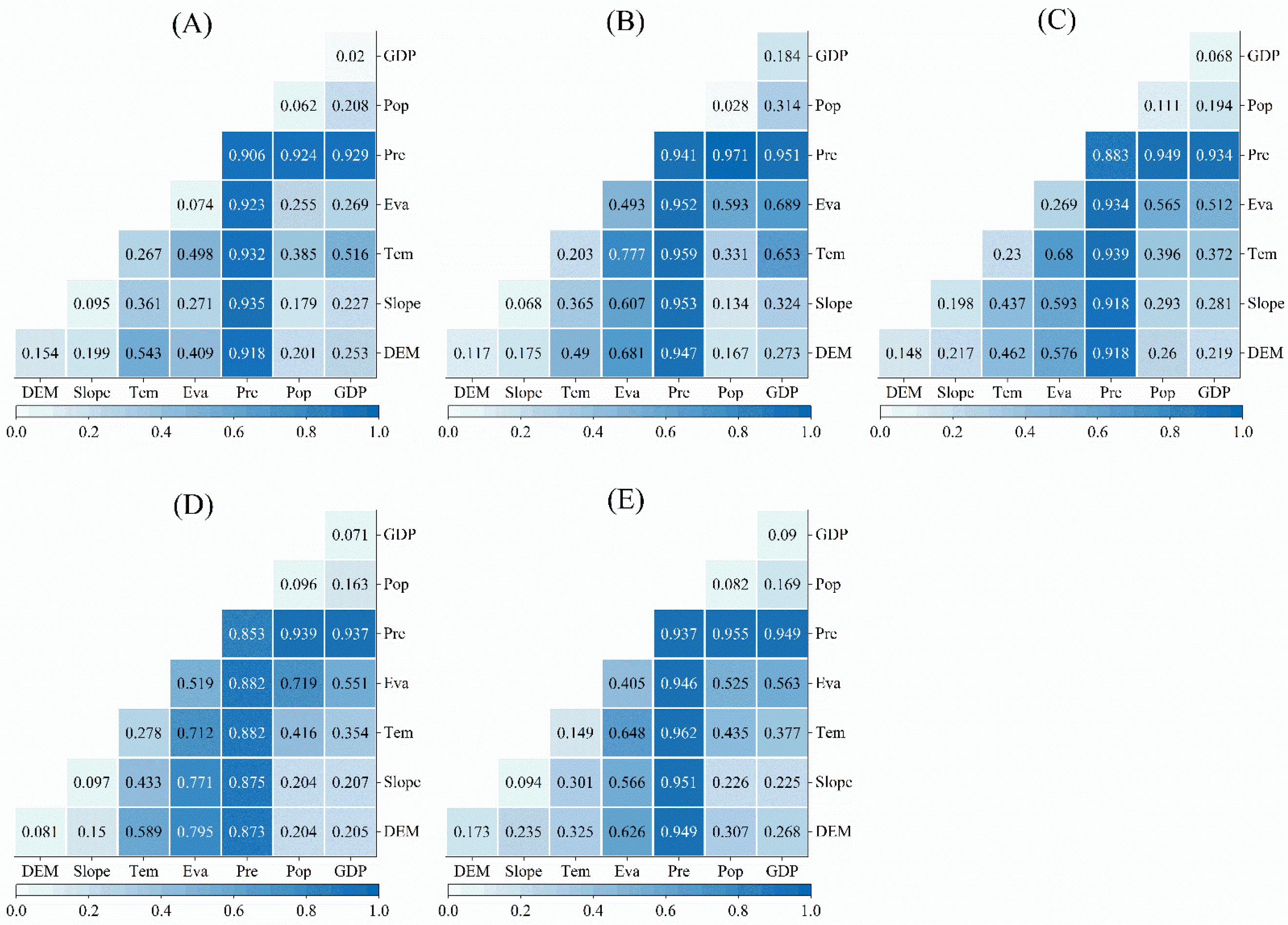
As shown in Figure 13, in studying the drivers of water yield changes in the Henan Yellow River Basin from 2000 to 2020, the interactions between two factors were stronger than the single-factor effects. In this study area, the interaction between mean annual precipitation and other factors has the highest explanatory power for the spatial variability of water yield, with q-values all greater than 0.873. Mean annual precipitation ∩ population density had the strongest explanatory power in 2005, 2010, and 2015. While they were not the strongest factors in 2000 and 2020, the q-values remained high at 0.924 and 0.955, respectively. The strongest explanatory powers in 2000 and 2020 were mean annual precipitation ∩ slope and mean annual precipitation ∩ mean annual temperature, respectively.
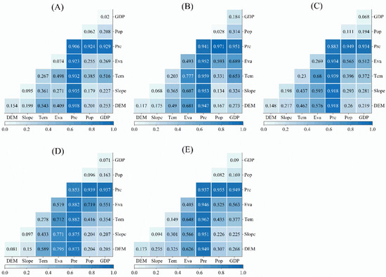
Figure 13.
Detection of the two-factor interaction affecting changes in water yield in the study area. (A) 2000; (B) 2005; (C) 2010; (D) 2015; (E) 2020.
It is observable that the interactions between mean annual precipitation and other factors have the greatest influence on changes in water yield. Natural and socioeconomic factors jointly influence water yield changes.
3.2.3. Analysis of Soil Conservation Drivers
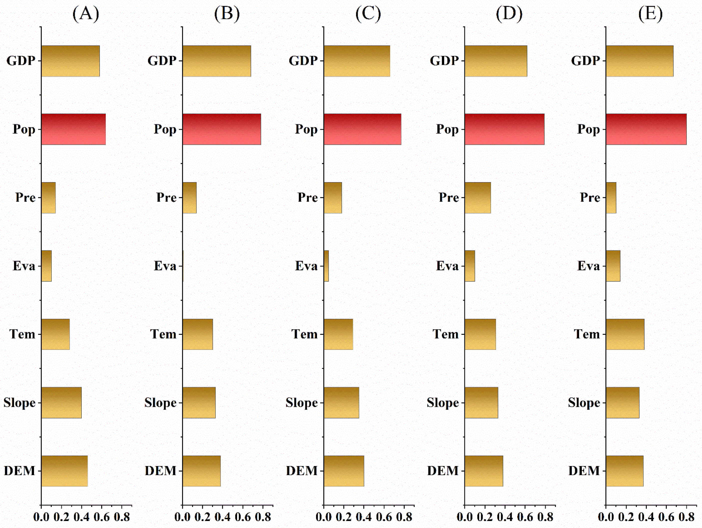
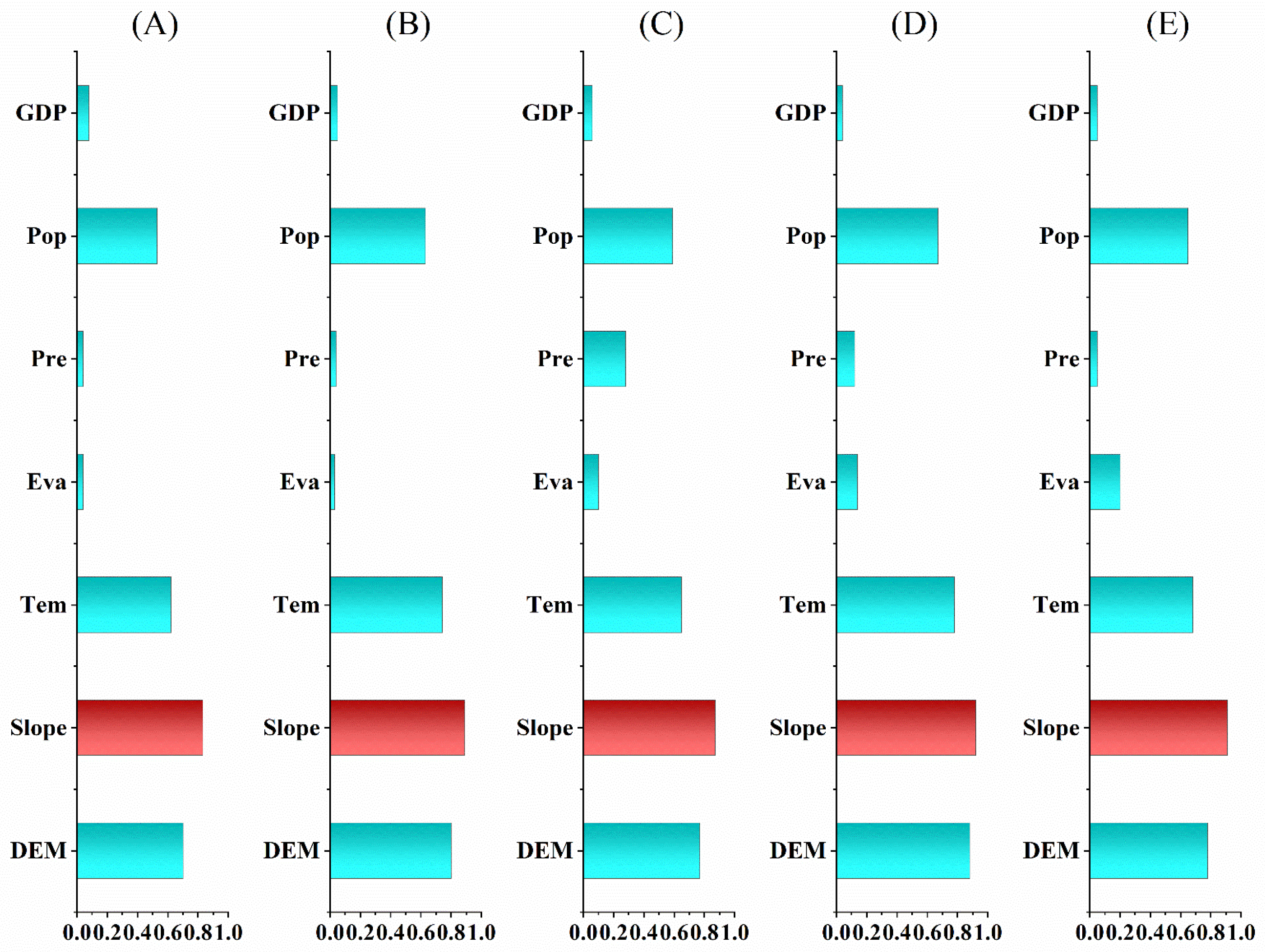
The average annual values of the driving factors from 2000 to 2020, ranked from highest to lowest by q-value, are as follows (Figure 14): slope (0.885) > elevation (0.784) > mean annual air temperature (0.694) > population density (0.615) > mean annual precipitation (0.105) > mean annual evapotranspiration (0.101) > GDP (0.058). The findings revealed that the slope, elevation, mean annual temperature and population density factors had a high impact on soil conservation changes, with the strongest explanatory power attributed to the slope factor, making it the main driver for soil conservation changes.
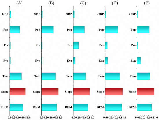
Figure 14.
Soil conservation driver q-values for the study area from 2000 to 2020. (A) 2000; (B) 2005; (C) 2010; (D) 2015; (E) 2020. Red: Indicates the highest q-value for the driving factor.
As shown in Figure 15, the interaction between slope and mean annual precipitation had the highest explanatory power for soil conservation variability from 2000 to 2020, which is consistent with the result that slope has the highest explanatory power for variations in soil conservation in one-factor detection. It is worth noting that the explanatory power of the interactions between average annual evapotranspiration and GDP and between average annual precipitation and GDP was low from 2000 to 2020. In 2010, the interpretative power of the interaction between mean annual precipitation and GDP increased slightly, with a q-value of 0.467 compared to 0.119 in 2005, consistent with the increased explanatory power of precipitation on soil conservation in 2010 in the one-way probe.
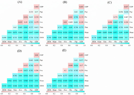
Figure 15.
Detection of two-factor interactions affecting soil conservation changes in the study area. (A) 2000; (B) 2005; (C) 2010; (D) 2015; (E) 2020.
In summary, slope, elevation, and average annual temperature are the main natural factors affecting soil conservation changes from 2000 to 2020, while population density is the key socioeconomic factor. These natural and socioeconomic factors collectively influence the spatial distribution of soil conservation.
4. Discussion
4.1. Methodological Limitations
The InVEST model and ArcGIS software (Version 10.8) were employed to quantitatively analyze the spatial and temporal features of carbon stock, water yield, and soil conservation ecosystem services in the Henan Yellow River Basin from 2000 to 2020, along with their evolution across different land use types in this research. Before this study, numerous scholars have utilized the InVEST model for ecosystem service assessments [59,60].
Nonetheless, the carbon stock assessment in the InVEST model primarily relies on land use type distributions and corresponding carbon density values for estimating carbon stock, streamlining the calculation process and enhancing efficiency to a certain extent [18]. However, it overlooks other influential factors such as soil conditions, topography, and climate, thereby compromising the accuracy of carbon stock estimates [19,20]. Biomass inversion methods could be integrated to refine vegetation carbon stock assessments and enhance module accuracy [41]. Biomass statistics for two forest types are presented in Table 10. Jia et al.’s research on tree forest vegetation carbon stock characteristics in Henan Province during 2008 and 2013 indicated carbon densities of approximately 24.62 t/ha and 24.31 t/ha, respectively, aligning closely with this study’s findings, considering tree biomass typically holds a carbon content of around 0.5, underscoring the reliability of biomass inversion outcomes in this study [61,62]. It has been demonstrated through existing studies that the overall results possess a certain degree of reliability. However, additional ground-truthing data may be required in the future to further enhance the scientific validity and accuracy of the results, thereby providing a more credible assessment.
Table 10.
Biomass density of different forest types (Unit: t/ha).
The use of Geodetector for analysis comes with certain limitations. The results obtained from Geodetector depend on the selection of driving factors. However, comprehensively covering all potential influencing factors can be challenging in practical research. In this study, common natural and socio-economic factors, including topography, climate change, population density, and GDP, were primarily considered. However, potentially significant factors such as vegetation types and land management policies may have been overlooked. Such limitations in factor selection may result in the underestimation or omission of certain influences, thereby impacting the comprehensiveness and accuracy of the results, indicating the need for future studies to include a broader range of factors.
This study focused primarily on carbon stock, water yield, and soil conservation, overlooking aspects like biodiversity, recreational amenities, and cultural values [63,64]. Future research should address these dimensions for a more holistic analysis.
4.2. Results Discussion
Ecosystem services assessment in the Henan Yellow River Basin from 2000 to 2020 reveals significant trends across carbon stock, water yield, and soil conservation. Carbon stock has steadily increased, with the most pronounced rise observed between 2005 and 2010, marking a 1.55% increase. This increase underscores the impactful role of the Grain for Green Project and China’s Natural Forest Conservation Project in Henan Province since 1998 [35,36]. In forested areas, consistent with findings from similar studies, it has been observed that these regions generally exhibit higher carbon sequestration capabilities [65]. Meanwhile, total water yield has exhibited a steady decline, dropping by 20.08% over the studied period, mirroring findings from Wei et al., who documented a 22.97% decrease in coastal areas of the Yellow River in Henan Province from 2000 to 2018 [66]. Soil conservation efforts from 2000 to 2020 revealed peak levels in 2010 followed by a decline in 2015, driven largely by rainfall patterns influencing erosion potential.
Geodetector analysis revealed that population density emerges as the principal socio-economic factor influencing spatial and temporal variations in carbon stock across the Henan Yellow River Basin. Additionally, natural factors such as DEM and slope exert significant influence, emphasizing the critical role of human activities in regional carbon sequestration dynamics. The Henan section, marked by population density and economic centrality in the province, faces heightened agricultural demands due to its dense population, impacting land use and soil carbon sequestration capacity [67]. Increased population density can prompt shifts in land use patterns, including agricultural expansion and urbanization, with varying impacts on carbon stock [68,69]. Hence, future development strategies should prioritize balanced population growth and comprehensive urban-rural planning policies to mitigate ecological impacts, especially in environmentally sensitive areas. Strengthening ecological restoration efforts in densely populated regions through initiatives such as afforestation, wetland preservation, and grassland restoration will be crucial for enhancing the region’s carbon sink capacity.
4.3. Socio-Ecological Implications
In the study area, comprehensive policy instruments should be adopted to protect and manage ecosystems, taking into account the joint influence of natural and socio-economic factors on ecosystem services.
In terms of spatiotemporal changes in ecosystem service functions, the ecological conservation policies implemented since 2000 in the Henan Yellow River Basin have yielded positive outcomes. Measures for example the Natural Forest Protection Project and the Grain for Green Project have notably improved ecosystem service quality. Despite these gains, the biomass of forests in Henan remains below the national average, indicating insufficient carbon sequestration capacity. Therefore, forest conservation efforts in the Henan Yellow River Basin should be strengthened, with continued implementation of policies such as the protection of natural forests and the conversion of farmland to forests. In areas with dense populations and frequent economic activities, increasing forest cover will enhance the carbon sink capacity of vegetation. Additionally, urban expansion and agricultural land use should be planned rationally to promote sustainable agricultural practices and a green economy, thereby reducing soil carbon emissions and minimizing damage to natural ecosystems from human activities.
The decline in water yield and soil conservation in the Henan Yellow River Basin indicates a need to further strengthen regional soil and water conservation capacity as well as soil erosion control. First, rainfall collection and water storage facilities should be enhanced to increase water yield, such as through the construction of reservoirs and berm projects. Additionally, water-saving irrigation techniques should be promoted, and green spaces should be increased in urban planning to enhance water conservation capacity. Research indicates that water yield is primarily influenced by rainfall, necessitating the strengthening of precipitation monitoring and early warning systems to rationalize water allocation strategies. Furthermore, strong support for environmentally friendly industries and green development techniques will be crucial in reducing water resource consumption by industrial and economic activities.
Soil conservation is most impacted by slope; therefore, vegetation planting should be increased on steep slopes, terraces should be constructed, and artificial slope reduction should be implemented on slopes unsuitable for planting and prone to landslides. Additionally, attention should be given to mountain soil restoration and ecosystem protection. Tree planting and grassland restoration should be prioritized in unutilized areas to improve vegetation coverage, increase the greening rate of barren mountains, and enhance the soil and water conservation functions of the Henan Yellow River Basin. Simultaneously, efforts should be made to enhance the relationship between economic development and the ecological environment, promote sustainable development, and advocate for the development of ecological and tourist agriculture as a means to optimize agricultural structure, improve the quality of the ecological environment, protect ecosystem services, and promote socio-economic development.
5. Conclusions
This study assessed the evolution and driving factors of ecosystem services in the Henan Yellow River Basin from 2000 to 2020, focusing on carbon stock, water yield, and soil conservation using the InVEST model and Geodetector. As hypothesized in the study, these ecosystem services have undergone certain changes in spatiotemporal scales, and these changes have been driven by topography, climate, land use, and socio-economic factors. The results are as follows:
- (1)
- The total carbon stock shows an increasing trend, going from 6.33 × 10⁸ t in 2000 to 6.45 × 10⁸ t in 2020. Total water yield showed a “falling-rising” pattern, with a low of 5.23 × 10¹⁰ m3 in 2015 and a peak of 7.37 × 10¹⁰ m3 in 2000. The total soil conservation exhibits a “decline-rise-decline-rise” pattern, with an overall decreasing trend.
- (2)
- The spatial distribution of the three ecosystem services has a high degree of consistency. The southwestern, central-eastern, and northern regions of the study area demonstrate better ecosystem service functions, with higher levels of carbon stock, water yield, and soil conservation. The land use distribution in these regions is predominantly forested.
- (3)
- Broad-leaved forests had the highest carbon stock per unit area, followed by coniferous forests. Coniferous and broad-leaved mixed forests ranked highest for water yield density. Soil conservation was highest in coniferous and broad-leaved mixed forests.
- (4)
- Population density primarily influenced changes in carbon stock. Water yield was mainly driven by precipitation, while soil conservation was most affected by slope. Population density ∩ DEM and precipitation provide the strongest explanatory power for carbon stock. The interaction between precipitation and other factors exhibits the highest explanatory power for water yield. Similarly, slope ∩ precipitation shows the greatest explanatory power for soil conservation.
Although this study provides valuable insights into ecosystem service changes and driving factors in the Henan Yellow River Basin, it has limitations. For example, the study’s uncertainty is influenced by the limitations of the InVEST model, the restricted availability of validation data, and the incomplete selection of driving factors. In conclusion, the study, supported by the optimized InVEST model and Geodetector, revealed that carbon stock, water yield, and soil conservation in the study area exhibited distinct spatial and temporal variations under the combined influences of topography, meteorology, land use, population, and socio-economic factors. The necessity of formulating a targeted regional ecological protection strategy is emphasized, providing a scientific reference for ecological restoration in the study area and offering methodological support for similar research.
Author Contributions
Conceptualization, X.W. and L.F.; methodology, X.W. and L.F.; software, L.F., R.C. and X.L.; validation, L.F. and X.W.; investigation, L.F. and Y.H.; resources, X.W.; data curation, X.L. and R.C.; writing original draft, L.F.; writing review and editing, X.W.; visualization, Y.H. and R.C.; supervision, X.W.; project administration, X.W., Z.C. and S.W.; funding acquisition, X.W., Z.C. and S.W. All authors have read and agreed to the published version of the manuscript.
Funding
This work was supported by the National Natural Science Foundation of China [grant No. 32371667].
Institutional Review Board Statement
Not applicable.
Informed Consent Statement
Not applicable.
Data Availability Statement
Data are contained within the article.
Conflicts of Interest
The authors declare no conflict of interest.
References
- Costanza, R.; d’Arge, R.; de Groot, R.; Farber, S.; Grasso, M.; Hannon, B.; Limburg, K.; Naeem, S.; O’Neill, R.V.; Paruelo, J.; et al. The value of the world’s ecosystem services and natural capital. Nature 1997, 387, 253–260. [Google Scholar] [CrossRef]
- Daily, G.C. Nature’s Services: Societal Dependence on Natural Ecosystems; Island Press: Washington, DC, USA, 1997. [Google Scholar]
- Ouyang, Z.; Wang, R.; Zhao, J. Ecosystem services and their economic valuation. Chin. J. Appl. Ecol. 1999, 635–640. [Google Scholar]
- Fu, B.; Zhou, G.; Bai, Y.; Song, C.; Liu, J.; Zhang, H.; Lv, Y.; Zheng, H.; Xie, G. The main terrestrial ecosystem services and ecological security in China. Adv. Earth Sci. 2009, 24, 571–576. [Google Scholar]
- Fu, S.; He, C.; Ma, J.; Wang, B.; Zhen, Z. Ecological environment quality of the Shanxi section of the Yellow River Basin under different development scenarios. Chin. J. Appl. Ecol. 2024, 35, 1337–1346. [Google Scholar]
- Miao, C.; Ai, S.; Zhao, J.; Shao, T.; Cui, Y.; Guo, X. Research on ecological protection and high-quality development strategy of the Yellow River Basin. Yellow River Civiliz. Sustain. Dev. 2021, 123–132. [Google Scholar]
- Dragicevic, A.; Lobianco, A.; Leblois, A. Forest planning and productivity-risk trade-off through the Markowitz mean-variance model. For. Policy Econ. 2016, 64, 25–34. [Google Scholar] [CrossRef]
- Birdsey, R.; Pregitzer, K.; Lucier, A. Forest Carbon Management in the United States. J. Environ. Qual 2006, 35, 1461–1469. [Google Scholar] [CrossRef] [PubMed]
- Marsh, G.P. Man and Nature: Or, Physical Geography as Modified by Human Action; C. Scribner: New York, NY, USA, 1864. [Google Scholar]
- Holdren, J.P.; Ehrlich, P.R. Human population and the global environment. Am. Sci. 1974, 62, 282–297. [Google Scholar] [PubMed]
- Huang, C.; Yang, J.; Zhang, W. Development of ecosystem services evaluation models: Research progress. Chin. J. Ecol. 2013, 32, 3360–3367. [Google Scholar]
- Babbar, D.; Areendran, G.; Sahana, M.; Sarma, K.; Sivadas, A. Assessment and prediction of carbon sequestration using Markov chain and InVEST model in Sariska Tiger Reserve, India. J. Clean. Prod. 2021, 278, 123333. [Google Scholar]
- Mushet, D.M.; Neau, J.L.; Euliss, N.H. Modeling effects of conservation grassland losses on amphibian habitat. Biol. Conserv. 2014, 174, 93–100. [Google Scholar] [CrossRef]
- Dashtbozorgi, F.; Hedayatiaghmashhadi, A.; Dashtbozorgi, A.; Ruiz–Agudelo, C.A.; Fürst, C.; Cirella, G.T.; Naderi, M. Ecosystem services valuation using InVEST modeling: Case from southern Iranian mangrove forests. Reg. Stud. Mar. Sci. 2023, 60, 102813. [Google Scholar] [CrossRef]
- Zhao, S.; Zhou, D.; Wang, D.; Chen, J.; Gao, Y.; Zhang, J.; Jiang, J. Ecosystem carbon storage assessment and multi-scenario prediction in the Weihe River Basin based on PLUS-InVEST model. Chin. J. Appl. Ecol. 2024, 35, 1–14. [Google Scholar]
- Dai, E.; Wang, Y. Spatial heterogeneity and driving mechanisms of water yield service in the Hengduan Mountain Region. Acta Geogr. Sin./Dili Xuebao 2020, 75, 607–619. [Google Scholar]
- Wu, J.; Zhang, L.; Peng, J.; Feng, Z.; Liu, H.; He, S. The integrated recognition of the source area of the urban ecological security pattern in Shenzhen. Acta Ecol. Sin. 2013, 33, 4125–4133. [Google Scholar]
- Yang, D.; Liu, W.; Tang, L.; Chen, L.; Li, X.; Xu, X. Estimation of water provision service for monsoon catchments of South China: Applicability of the InVEST model. Landsc. Urban Plan. 2019, 182, 133–143. [Google Scholar] [CrossRef]
- Wang, R.-Y.; Mo, X.; Ji, H.; Zhu, Z.; Wang, Y.-S.; Bao, Z.; Li, T. Comparison of the CASA and InVEST models’ effects for estimating spatiotemporal differences in carbon storage of green spaces in megacities. Sci. Rep. 2024, 14, 5456. [Google Scholar] [CrossRef]
- Kohestani, N.; Rastgar, S.; Heydari, G.; Jouibary, S.S.; Amirnejad, H. Spatiotemporal modeling of the value of carbon sequestration under changing land use/land cover using InVEST model: A case study of Nour-rud Watershed, Northern Iran. Environ. Dev. Sustain. 2024, 26, 14477–14505. [Google Scholar] [CrossRef]
- Bai, X.M.; Shi, P.J.; Liu, Y.S. Realizing China’s urban dream. Nature 2014, 509, 158–160. [Google Scholar] [CrossRef]
- Yu, Y.Q.; Huang, Y.; Zhang, W. Modeling soil organic carbon change in croplands of China, 1980–2009. Glob. Planet. Chang. 2012, 82–83, 115–128. [Google Scholar] [CrossRef]
- Bryan, B.A.; Gao, L.; Ye, Y.Q.; Sun, X.F.; Connor, J.D.; Crossman, N.D.; Stafford-Smith, M.; Wu, J.G.; He, C.Y.; Yu, D.Y.; et al. China’s response to a national land-system sustainability emergency. Nature 2018, 559, 193–204. [Google Scholar] [CrossRef] [PubMed]
- Ouyang, Z.; Zheng, H.; Xiao, Y.; Polasky, S.; Liu, J.; Xu, W.; Wang, Q.; Zhang, L.; Xiao, Y.; Rao, E.M.; et al. Improvements in ecosystem services from investments in natural capital. Science 2016, 352, 1455–1459. [Google Scholar] [CrossRef]
- Xi, J. Speech at the Symposium on ecological protection and quality development of the Yellow River basin China. China Water Resour. 2019, 70, 1–3. [Google Scholar] [CrossRef]
- Jin, F. Coordinated promotion strategy of ecological protection and high-quality development in the Yellow River Basin. Reform 2019, 32, 33–39. [Google Scholar]
- Shen, J.; Zhao, M.; Tan, Z.; Zhu, L.; Guo, Y.; Li, Y.; Wu, C. Ecosystem service trade-offs and synergies relationships and their driving factor analysis based on the Bayesian belief Network: A case study of the Yellow River Basin. Ecol. Indic. 2024, 163, 112070. [Google Scholar] [CrossRef]
- Zhang, K.; Fang, B.; Zhang, Z.; Liu, T.; Liu, K. Exploring future ecosystem service changes and key contributing factors from a “past-future-action” perspective: A case study of the Yellow River Basin. Sci. Total Environ. 2024, 926, 171630. [Google Scholar] [CrossRef]
- Yu, Y.; Xiao, Z.; Bruzzone, L.; Deng, H. Mapping and analyzing the spatiotemporal patterns and drivers of multiple ecosystem services: A case study in the Yangtze and Yellow River Basins. Remote Sens. 2024, 16, 411. [Google Scholar] [CrossRef]
- Pang, C.; Wen, Q.; Ding, J.; Wu, X.; Shi, L. Ecosystem services and their trade-offs and synergies in the upper Yellow River Basin. Acta Ecol. Sin. 2024, 44, 5003–5013. [Google Scholar]
- Liu, J.; Wang, G.; Fu, X.; Yu, S.; Ren, M.; Shi, H.; Deng, X.; Chen, K. Evaluation of ecological protection and high-quality development level in Henan Section of the Yellow River Basin. Yellow River 2023, 45, 7–13. [Google Scholar]
- Zhang, C.; Wang, G. Thoughts on ecological protection and high-quality development in the Yellow River Basin. Yellow River 2024, 46, 1–7. [Google Scholar]
- Wang, X. Coordinating the promotion of ecological protection and management of the Yellow River and high-quality development of the entire basin. China Ecol. Civiliz. 2019, 7, 70–72. [Google Scholar]
- Yin, H. Ecological protection and sustainable economic development strategies of the Yellow River Basin. Soc. Sci. 2021, 36, 98–102. [Google Scholar] [CrossRef]
- Li, S.; Jin, M. World-Renowned Ecological Project—China’s “Natural Forest Conservation Project”; Zhejiang Forestry: Hangzhou, China, 2021; pp. 16–18. [Google Scholar]
- Zhao, J.; Yang, Y.; Wan, W.; Zhu, K.; Zhou, H.; Xu, Q. Monitoring and evaluation of effectiveness of Returning Grain Plots to Forest Project in Henan Province. J. Henan For. Sci. Technol. 2022, 42, 26–29. [Google Scholar]
- Wang, X. Analysis and forecast of Socio-Economic development in Henan Province. China Circ. Econ. 2020, 35, 82–84. [Google Scholar] [CrossRef]
- Wang, K.; Li, X.; Lyu, X.; Dang, D.; Dou, H.; Li, M.; Liu, S.; Cao, W. Optimizing the land use and land cover pattern to increase its contribution to carbon neutrality. Remote Sens. 2022, 14, 4751. [Google Scholar] [CrossRef]
- Jiang, L. Analyses of the Changes of Land Use and Carbon Stocks in Terrestrial Ecosystem of the Central Plains Economic Region from 2000 to 2020. Master’s Thesis, Henan University, Kaifeng, China, 2015. [Google Scholar]
- Zhang, L.; Dawes, W.R.; Walker, G.R. Response of mean annual evapotranspiration to vegetation changes at catchment scale. Water Resour. Res. 2001, 37, 701–708. [Google Scholar] [CrossRef]
- Hao, J.; Kangting, L.; Hu, T.; Wang, Y.; Xu, G. Remote sensing inversion of mangrove biomass based on machine learning. For. Grassl. Resour. Res. 2024, 46, 65–72. [Google Scholar] [CrossRef]
- Liu, Q.; Yang, L.; Liu, Q.; Li, J. Review of forest above ground biomass inversion methods based on remote sensing technology. Natl. Remote Sens. Bull. 2015, 19, 62–74. [Google Scholar]
- Liu, C.F.; Chen, D.H.; Zou, C.; Liu, S.S.; Li, H.; Liu, Z.H.; Feng, W.T.; Zhang, N.M.; Ye, L.Z. Modeling biomass for natural subtropical secondary forest using multi-source data and different regression models in Huangfu Mountain, China. Sustainability 2022, 14, 13006. [Google Scholar] [CrossRef]
- Liu, Y.; Shao, Z.; Wu, C.; Qi, X. Remote sensing estimation of vegetation above-ground biomass in Nachang based on GF-6 Image. J. Geomat. 2024, 49, 107–112. [Google Scholar]
- National Forestry and Grassland Administration. Guideline on Carbon Stock Accounting in Forest Ecosystem; Standards Press of China: Beijing, China, 2018; p. 16. [Google Scholar]
- Fang, J.; Liu, G.; Xu, S. Biomass and NET production of forest vegetation in China. Acta Ecol. Sin. 1996, 16, 497–508. [Google Scholar]
- Li, H. Accurate Estimate of Soil Organic Carbon Storage in Henan Province Based on High-Density Profiles. Master’s Thesis, Zhengzhou University, Zhengzhou, China, 2016. [Google Scholar]
- Wang, J.; Xu, C. Geodetector: Principles and prospects. Acta Geogr. Sin. 2017, 72, 116–134. [Google Scholar]
- Gao, W.; Du, Y.; Zhu, D.; Wan, L. Spatio-temporal evolution characteristics and driving mechanism of wetlands in Xiaoxing’an Mountains. Acta Ecol. Sin. 2024, 44, 1–16. [Google Scholar]
- Chen, J.H.; Wang, D.C.; Li, G.D.; Sun, Z.C.; Wang, X.; Zhang, X.; Zhang, W. Spatial and temporal heterogeneity analysis of water conservation in Beijing-Tianjin-Hebei urban agglomeration based on the Geodetector and Spatial Elastic Coefficient Trajectory Models. GeoHealth 2020, 4, e2020GH000248. [Google Scholar] [CrossRef]
- Ngabire, M.; Wang, T.; Liao, J.; Sahbeni, G. Quantitative analysis of desertification-driving mechanisms in the Shiyang River Basin: Examining interactive effects of key factors through the Geographic Detector Model. Remote Sens. 2023, 15, 2960. [Google Scholar] [CrossRef]
- Chen, S.; Jin, Y.; Huang, Y. Spatio-temporal variations of habitat quality and its underlying mechanism in the central region of Yangtze River Delta. Chin. J. Ecol. 2023, 42, 1175–1185. [Google Scholar]
- Yang, J.; Xie, B.; Zhang, D. Spatial-temporal evolution of habitat quality in the Yellow River Basin and its influencing factors. J. Desert Res. 2021, 41, 12–22. [Google Scholar]
- Bai, X.; Zhang, Z.; Li, Z.; Zhang, J. Spatial heterogeneity and formation mechanism of eco-environmental quality in the Yellow River Basin. Sustainability 2023, 15, 10878. [Google Scholar] [CrossRef]
- Li, C.; Qiao, W.; Chen, G. Unveiling spatial heterogeneity of ecosystem services and their drivers in varied landform types: Insights from the Sichuan-Yunnan ecological barrier area. J. Clean. Prod. 2024, 442, 141158. [Google Scholar] [CrossRef]
- Ling, M.; Chen, J.; Lan, Y.; Chen, Z.; You, H.; Han, X.; Zhou, G. Exploring the drivers of soil conservation variation in the source of Yellow River under diverse development scenarios from a geospatial perspective. Sustainability 2024, 16, 777. [Google Scholar] [CrossRef]
- Liu, C.; Zou, L.; Xia, J.; Chen, X.; Zuo, L.; Yu, J. Spatiotemporal heterogeneity of water conservation function and its driving factors in the Upper Yangtze River Basin. Remote Sens. 2023, 15, 5246. [Google Scholar] [CrossRef]
- Li, N.; Sun, P.; Zhang, J.; Mo, J.; Wang, K. Spatiotemporal evolution and driving factors of ecosystem services’ transformation in the Yellow River basin, China. Environ. Monit. Assess. 2024, 196, 252. [Google Scholar] [CrossRef] [PubMed]
- Zhang, P.; Liu, S.; Zhou, Z.; Liu, C.; Xu, L.; Gao, X. Supply and demand measurement and spatio-temporal evolution of ecosystem services in Beijing-Tianjin-Hebei Region. Acta Ecol. Sin. 2021, 41, 3354–3367. [Google Scholar]
- Liu, Y.; Zhang, J.; Zhou, D.; Ma, J.; Dang, R.; Ma, J.; Zhu, X. Temporal and spatial variation of carbon storage in the Shule River Basin based on InVEST model. Acta Ecol. Sin. 2021, 41, 4052–4065. [Google Scholar]
- Jia, S. Study on carbon storage of forest vegetation and its economic value in Henan Province based on continuous forest resources inventory. Hubei Agric. Sci. 2016, 55, 1612–1616. [Google Scholar]
- Jia, S.; Guo, M. Carbon storage characteristics of arboreal forests vegetation of Henan Province in 2013. Res. Soil Water Conserv. 2019, 26, 29–34. [Google Scholar]
- Biber, P.; Felton, A.; Nieuwenhuis, M.; Lindbladh, M.; Black, K.; Bahyl, J.; Bingöl, Ö.; Borges, J.G.; Botequim, B.; Brukas, V.; et al. Forest biodiversity, carbon sequestration, and wood production: Modeling synergies and trade-offs for ten forest landscapes across Europe. Front. Ecol. Evol. 2020, 8, 547696. [Google Scholar] [CrossRef]
- Schulp, C.J.E.; Nabuurs, G.J.; Verburg, P.H. Future carbon sequestration in Europe—Effects of land use change. Agric. Ecosyst. Environ. 2008, 127, 251–264. [Google Scholar] [CrossRef]
- Pan, Y.; Birdsey, R.A.; Fang, J.; Houghton, R.; Kauppi, P.E.; Kurz, W.A.; Phillips, O.L.; Shvidenko, A.; Lewis, S.L.; Canadell, J.G.; et al. A large and persistent carbon sink in the world’s forests. Science 2011, 333, 988–993. [Google Scholar] [CrossRef]
- Wei, H.; Xue, D.; Huang, J.; Liu, M.; Li, L. Identification of coupling relationship between ecosystem services and urbanization for supporting ecological management: A case study on areas along the Yellow River of Henan Province. Remote Sens. 2022, 14, 2277. [Google Scholar] [CrossRef]
- Zhang, X.; Yang, W.; Xu, Y. Effects of main tillage methods on soil structure, nutrients and micro-ecological environment of upland in China: A review. Ecol. Environ. Sci. 2019, 28, 2464–2472. [Google Scholar]
- Liang, D.Z.; Lu, H.W.; Guan, Y.L.; Feng, L.Y.; He, L.; Qiu, L.H.; Lu, J.Z. Population density regulation may mitigate the imbalance between anthropogenic carbon emissions and vegetation carbon sequestration. Sustain. Cities Soc. 2023, 92, 104502. [Google Scholar] [CrossRef]
- Chien, S.C.; Knoble, C.; Krumins, J.A. Human population density and blue carbon stocks in mangroves soils. Environ. Res. Lett. 2024, 19, 034017. [Google Scholar] [CrossRef]


Disclaimer/Publisher’s Note: The statements, opinions and data contained in all publications are solely those of the individual author(s) and contributor(s) and not of MDPI and/or the editor(s). MDPI and/or the editor(s) disclaim responsibility for any injury to people or property resulting from any ideas, methods, instructions or products referred to in the content. |
© 2024 by the authors. Licensee MDPI, Basel, Switzerland. This article is an open access article distributed under the terms and conditions of the Creative Commons Attribution (CC BY) license (https://creativecommons.org/licenses/by/4.0/).