Abstract
Chestnut (Castanea sativa Mill.) forests in the Mediterranean region are facing increasing abandonment due to a combination of factors, ranging from climate change to socioeconomic issues. The recovery of chestnut ecosystems and their preservation and valorization are key to ensuring the supply of the wide spectrum of ecosystem services they provide and to preventing detrimental environmental shifts. The study’s objective was to provide evidence on the effects of different management options on the ecophysiology of chestnut forests, with diverse pruning intensities (low, medium, and high intensity versus no pruning) tested in an abandoned chestnut stand in central Italy with the aim of recovering and rehabilitating it for fruit production. Innovative Internet of Things (IoT) ‘Tree Talker’ devices were installed on single trees to continuously monitor and measure ecophysiological (i.e., water transport, net primary productivity, foliage development) and microclimatic parameters. Results show a reduction in water use in trees subjected to medium- and high-intensity pruning treatments, along with a decrease in the carbon sequestration function. However, interestingly, the results highlight that trees regain their usual sap flow and carbon sink activity at the end of the first post-pruning growing season and fully realign during the following year, as also confirmed by the NDVI values. As such, this paper demonstrates the efficacy of recovering and managing abandoned chestnut forests, and the initial setback in carbon sequestration resulting from pruning is rapidly remedied with the advantage of reviving trees for fruit production. Additionally, the reduced water demand induced by pruning could represent a promising adaptation strategy to climate change, bolstering the resilience of chestnut trees to prolonged and intensified drought periods, which are projected to increase under future climate scenarios, particularly in the Mediterranean region.
1. Introduction
Sweet chestnut (Castanea sativa Mill.) is distributed throughout Europe and Western Asia, where, for centuries, it has been considered economically relevant to human interest in wood and fruit production. In Europe, chestnut forests cover more than 2.5 million hectares of land [1] and are found in natural and semi-natural stands, as well as in managed stands, including orchards and plantations, where proper silvicultural and management practices are applied to ensure high levels of wood or fruit production [2,3]. Chestnut stands provide several ecosystem services, including a provision (e.g., wood and biomass production, food including fruits and flour, tannin), regulation (e.g., carbon sequestration and climate regulation, biodiversity protection, water quality, erosion control, and soil disturbance prevention), and cultural services (e.g., aesthetic landscape, sense of place, and traditional knowledge) [3,4,5,6]. In Italy, chestnut forests occupy almost 10% of the national forest lands [7] and, from ancient times, act as a major economic source for rural populations in mountain Apennine regions, where cultivation of chestnuts is considered an old tradition by the native population.
Italy is the main European producer of chestnut wood and fruits. Specifically, it is the fourth country in terms of chestnut fruit production worldwide, with a potential annual supply of approximately 55,000 tons on average, which amounts to a basic economic value of 60–65 million euros, supported also by the recognized high-quality standards of Protected Designation of Origin (PDO) and Protected Geographical Indication (PGI) fruits, which can increase to as much as 165 million euros if considering the whole value chain, including woodland by-products, timber, and the tourist appeal of these areas of high historical and cultural heritage value [8,9,10].
Nevertheless, nowadays, chestnut forests in Italy are experiencing an increasing abandonment, turning into unmanaged woodland [8,9,10]. This is due to a combination of factors ranging from climate change, which increases the occurrence of pests and diseases directly impacting chestnut wood and fruit production [11] with significant reduction in yields, thus making cultivation more challenging, to socioeconomic factors, such as the aging of the rural population with consequent depopulation of many rural areas, resulting in the loss of specialized knowledge and skills, decline in the agricultural workforce, and a lack of manpower to maintain and cultivate chestnut trees, reducing the profitability of domestic chestnut forests and making imported chestnuts more competitive in the market, particularly in countries with lower production costs [8,9,10].
The recovery of the chestnut ecosystems and their valorization and preservation are key to ensuring the supply of the wide spectrum of ecosystem services they provide and to avoiding hazardous environmental shifts [12], including changing phenological patterns due to climate change, as also occurring for other species [13], as well as to revive and maintain the contribution to the development of the local economy [14], as well as possible sustainable and circular economy approaches as demonstrated for the agricultural sector [15]. This can be achieved by implementing proper practices to manage chestnut forests. Pruning is a relevant management practice historically carried out, particularly in orchards and plantations, with the aim of improving tree shape and increasing its strength, reducing stems or branch breakage, particularly after strong winds [16]; it also enhances tree growth and fruit production [17].
Chestnut ecosystems have been widely investigated in the literature, with studies discussing the impacts of climate change [18], including new emerging diseases [11] and ways to contrast them [19], identifying the most suitable areas for their growth [20], evaluating the effect of management practices on the chestnuts’ nutrient budget [21], on soil disturbance [22], on their production in terms of fruit characteristics [23], and assessing how management options can improve the quality of wood production [24,25] or restore chestnut stands damaged by pests [26]. Some contributions in the literature [27,28] suggest that the productive capacity of Castanea sativa species increases when receiving periodic pruning, and the recovery of abandoned chestnut forests in Italy also improves soil microbial activities and organic carbon content [29,30]. Other studies demonstrated for some forest and orchard tree species other than chestnut that pruning can have positive effects on fruit and wood production [18,31,32,33,34] in natural or urban environments, with effects on tree growth and its physiological processes [35,36], including daily water use in terms of sap flow [37], transpiration [38,39], photosynthetic activity, and consequently the carbon sequestration potential [40]. However, the effects of the conversion of abandoned chestnut forests into managed ones remain scarcely investigated, particularly in relation to their main ecophysiological characteristics, although they can also reflect the influence of interannual and seasonal variations [1,2,17].
Against this backdrop, this paper provides evidence on a current research gap using for the first time in chestnut stands innovative Internet of Things (IoT) Tree Talker (TT) devices to continuously measure ecophysiological and microclimatic parameters of single trees, as recently demonstrated by Niccoli et al. [41] to determine the effect of wildfire on Pinus pinaster and by Asgharinia et al. [42] to evaluate stem water dynamics in Fagus sylvatica L. and Quercus petraea L. Specifically, with the aim to recover an abandoned chestnut forest and combine fruit production and ecosystem services provision, different pruning treatments were tested in a forest plot in the Apennine of central Italy, and their effects on the trees’ growth and ecophysiology were monitored by using a set of IoT sensors combined into single Tree Talker devices. The study’s objective is to determine, compare, and evaluate the ecophysiological forest response to different pruning intensities in terms of water transport, net primary productivity, carbon sequestration, foliage development, and canopy health to calibrate management practices and detect the most promising based on the multifunctionality of the chestnut forest ecosystem, including possible effects on coping with climate change mitigation and adaptation.
2. Materials and Methods
2.1. Study Area
The study was carried out in an experimental-educational area in a chestnut belt of Apennine Forest, northern Italy (Granaglione, Alto Reno Terme, Bologna, Italy) at an altitude of about 700 m above sea level. The experimental site is an 11 ha pure stand of chestnut trees (Castanea sativa Mill), about 75 years old, growing on a Leptic Skeletic Dystric Regosols (Loamic, Humic) soil type [43] with a pedological substrate characterized by arenaceous rocks in detrital facies (located at the coordinates 44°8′24″ N, 10°57′27″ E). The stand has been owned since 2003 by “Fondazione Cassa di Risparmio di Bologna” and was traditionally managed with regular pruning of trees with the scope of chestnut fruit production, but abandoned in the last decade mainly due to socioeconomic factors, such as aging of the rural population and consequent land abandonment, lack of specialized knowledge and skills, and market competition with imported chestnuts. Recently, thanks to the commitment of the National (Italian) Academy of Agriculture since 2016, new experimental activities have begun, and the stand is currently a National Center for the Study and Conservation of Forest Biodiversity according to the Law Decree of the Italian Ministry of the Environment. In this context, with the aim of recovering the abandoned chestnut forest and rehabilitating it for fruit production, in February 2020, four pruning treatments with different intensities were carried out. The effects were monitored on 12 chestnut trees (Figure 1) distributed in an 800 m2 area and selected with similar diameters ranging from 31.83 to 55.70 cm to reduce potential side effects related to tree dimension—see Table 1 with the main attributes of selected trees. The four pruning treatments, each replicated four times, were as follows:
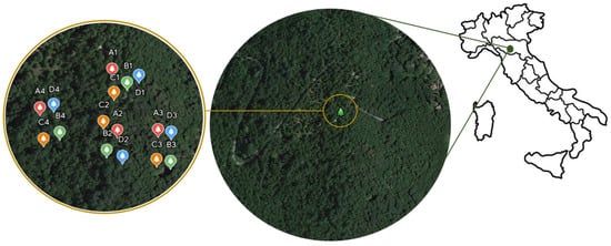
Figure 1.
Map of the study area showing the localization of selected chestnut trees. Red marks (group A) represent intensely pruned trees, green marks (group B) represent medium-pruned trees, orange marks (group C) represent low-pruned trees, and blue marks (group D) represent control, not pruned trees.

Table 1.
Characteristics of the selected trees pruned at different intensities.
- −
- Intense pruning, with the removal of the 1st order branches or topping,
- −
- Medium pruning, with the removal of the 2nd order branches,
- −
- Low pruning, with the removal of the 3rd order branches or topping,
- −
- No pruning, which was the control.
According to [44], the sapwood area A(sap) is calculated in relation to the stem cross-sectional area at breast height A(stem) using the following equation for broadleaf ring-porous trees:
where “a” and “b” are allometric parameters equal to 0.2509 and 0.9259, respectively.
A(sap) = a × A(stem)b
2.2. The Tree Talker System
A set of Internet of Things (IoT) sensors combined into single Tree Talker (TT) devices was installed on the selected 12 chestnut trees at breast height in May 2020, with the aim of monitoring the effects of different pruning treatments on the main ecophysiological parameters during two consecutive growing seasons in 2020 and 2021.The Tree Talker is an Internet of Things (IoT) device recently developed [45,46] to measure, at an hour time step and simultaneously, important ecophysiological and microclimatic parameters on a single tree scale. The key parameters measured by the Tree Talker for the purposes of this study are:
- −
- Air relative humidity (%) and air temperature (°C) were measured by a thermo-hygrometer.
- −
- Sap flux density and sap flow were measured using an electrically heated probe, serving as a heat dissipation sensor, and an unheated probe, serving as a reference, using the transient thermal dissipation method [47,48].
- −
- Canopy light transmission was measured by a spectrometer at 12 spectral bands (450, 500, 550, 570, 600, 610, 650, 680, 730, 760, 810, and 860 nm).
Moreover, in addition to the 12 Tree Takers, an additional TT-solar was installed in a fully exposed position in an open space in the vicinity of the chestnut forest to obtain real-time information on total solar irradiance, which was measured for the same 12 spectral bands of the TT. The spectrometer was manufactured as directly embedded into the TT device by integrating into a single board the AMS Osram (https://ams-osram.com/ accessed on 30 August 2024) chipset AS7262 (Visible range) and AS7263 (Near Infra-Red range), with a Full Width Half Maximum (FWHM) of ±10 nm for the visible and ±20 nm for the near infra-red bands. The spectrometer communicates with the microprocessor Tree Talker unit by an I2C interface.
Each Tree Talker is equipped with a rechargeable battery powered by a solar panel. The TT acquires hourly signals in the form of digital numbers from all its sensor components and stores them in a data logger and, at the same time, it transmits the same information to a TT-Cloud through the Long Range (LoRa) protocol, which is a low-power wide-area network modulation technique. Then, the TT-Cloud uses a GPRS signal to transfer data to a computer server via GSM/GPRS technology. Thus, a unique IoT identifier allows us to follow the individual tree life along its development from hours to season and the interannual time scale.
2.3. Measurement of Sap Flow and VPD
Measuring sap flow, which is a function of the transpiration rate measured as the ascent of sap within xylem tissue [49,50,51,52], is important for understanding water transport in the soil-plant-atmosphere system because it indicates the amount of water absorbed by the plant and potentially transpired [53]. In fact, the transpiration rate of the plant system can be closely approximated by the sap flow rate in the main stem or trunk [45].
To measure sap flow, a thermal-based method [47,48] was used because it possesses many advantages over other methods and has become the most widely used approach to estimate forest transpiration at both the individual tree and stand scales [54,55,56]. To this end, TT devices are equipped with a heated and a reference probe for the application of the thermal dissipation method originally developed by Granier [48] and modified according to Do et al. [47] to reduce the energy consumption due to continuous heating. In fact, the Granier [48] the original method calculates the sap flux density (i.e., the volume of sap flowing across a given area of sapwood per unit of time) based on the assessment of the amount of heat dissipated from a heated probe in relation to a reference probe in proximity, with continuous heating. To reduce energy consumption in the TT device—thus lengthening battery duration and reducing field interventions for battery recharge—the continuous heating method was modified according to Do et al. [47] with cycles of cooling (50 min) and heating (10 min).
The TT heated and reference probes are installed in the tree stem at a vertical distance of 10 cm from each other. Probes have a diameter of 2.5 mm each and are positioned at a depth of 2.5 cm in the sapwood of the selected trees, at the breast height (about 1.3 m), with a northerly orientation well protected from direct sun heating and measured the sapwood heat dissipation, which increases with sap velocity that has the effect of cooling the heat source [41,42]. When the sap velocity is zero or minimal, the temperature difference (ΔT) between the two sensors is maximal. When the flow increases, the temperature difference decreases. However, many factors influence the sap flow measurement, such as the tree’s diameter and stem uniformity [57], and the sap velocity varies within the sapwood [57,58,59]; therefore, parameters like sapwood thickness can introduce some uncertainty in the sap flow assessment [60]. In this study, sap flow (i.e., the integration of sap flux across the entire conducting wood or sapwood in a tree, expressed as the volume of sap over a day) was calculated with the assumption that the whole trunk sapwood area was conducting water homogeneously. The sapwood area was determined according to [44], as previously explained in Section 2.1.
Sap flow is calculated based on the parameters recorded by the Tree Talkers using the heat dissipation method developed by Granier [48] and modified by Do et al. [47], whose formula was further adjusted by the TT developer with coefficients according to the characteristics of the material used to manufacture the heating probe (Nature 4.0 Manual, 2023). Thus, sap flux density (SFD) is calculated using the following equation:
where:
SFD is sap flux density (g m−2 s−1),
ΔT is the temperature difference between the heated and unheated probe,
ΔTmax is the maximum temperature gradient measured between the probes after heating within 24 h, which usually occurs during the nighttime in the case of zero transpiration and zero tree-body refilling [53].
Assuming that the SFD is constant across the sapwood profile, the sap flow (SF) can be calculated according to Santiago et al. [61] and Oren & Pataki [62] as:
where:
SF is sap flow (L d−1),
A(sap) is the sapwood area of a chestnut tree.
The main environmental controls of tree water use are global radiation, soil water availability, and atmospheric vapor pressure deficit (VPD) [53,63]. VPD is a measure of the difference between the amount of moisture in the air and the maximum amount of moisture the air can hold at a given temperature [64]. It is commonly used to estimate the evaporative demand of the atmosphere. In fact, the impact of VPD on tree water use is the result of the leaf–atmosphere vapor pressure difference, which creates water suction. This force usually acts as the main driver of water transport in plants. Several studies have shown that high VPD generally leads to increased transpiration and sap flow; however, when VPD is above a certain level, stomatal conductance may decline [65,66], causing a reduction in tree water use [67].
VPD (kPa) is calculated according to [68]:
where:
a, b, and c are constant parameters, i.e., 0.611 kPa, 17.502 (unitless), and 240.97 °C, respectively,
RH is relative air humidity (%), measured by TT
T is the air temperature (°C), measured by TT.
The VPD was assessed in this study to evaluate its correlation with sap flow on a daily basis using the Pearson correlation.
2.4. Light-Use Efficiency for Estimating Net Primary Productivity
Estimating net primary productivity (NPP) is essential for understanding the carbon balance, predicting ecosystem responses to environmental changes, and informing sustainable land management [69,70,71]. Although NPP of forest ecosystems is usually assessed using remote-sensed data [72,73], in this study, it was estimated using data collected through in-situ sensors and light use efficiency (LUE) models, which are also widely used around the world to estimate forest net primary productivity [74,75,76,77]. In fact, NPP is strongly dependent on solar radiation and plays an important role in vegetation growth, providing essential energy for photosynthetic activities [78,79]. In the past decades, many LUE models have been built [77] to estimate terrestrial productivity based on the rationale that daily photosynthesis is proportional to Absorbed Photosynthetic Active Radiation (APAR) according to the Monteith theory [78]. The LUE approach for estimating NPP is built upon two fundamental assumptions [80]: (1) the ecosystem productivity is directly related to the absorbed photosynthetically active radiation (APAR) through LUE, where the photosynthetically active radiation (PAR) is the spectral range of solar radiation from 400 to 700 nanometers that photosynthetic organisms are able to use in the process of photosynthesis, and LUE is defined as the amount of carbon produced per unit of APAR; and (2) the realized LUE may be reduced below its theoretical potential value due to environmental stresses such as low temperatures or water shortages. According to Landsberg [81], the general formula for the LUE model is:
where:
NPPabg = Ɛ × Φabs
NPPabg is the net primary production in the above-ground biomass (g of dry matter m−2),
Φabs is the amount of PAR absorbed by a canopy (MJ m−2),
Ɛ is the light-use efficiency (g of dry matter MJ−1).
The concept of light-use efficiency has been the subject of various experimental and theoretical studies, and various authors have provided empirical determinations of Ɛ for different forest types [81]. According to Gower et al. [82], for temperate deciduous forests, Ɛ is assumed to be 0.65 g of dry matter MJ−1.
The total solar radiation and solar radiation transmitted by the canopy of each tree are directly measured as digital numbers (DNs) for 12 spectral bands by the TT-solar and by the TreeTalkers, respectively (see Section 2.2). According to Doughty et al. [83] and Ollinger [84], canopy reflectance in the visible region (400 nm to 700 nm) is typically around 5%–15% for broadleaves. Therefore, we can assume that the canopy of a chestnut tree generally reflects, on an average, 10% of the received visible radiation. Consequently, the energy absorbed by the canopy of a tree can be calculated as the normalized (N) difference between 90% of the total solar radiation (measured by the TT-solar) and the solar radiation transmitted by the canopy of each tree (measured by the TTs).
Therefore, the following expression is used:
and then:
N(Absorbed + Reflected) = 1 − (DN(TT)/DN(TT-solar))
N(Absorbed) = DN(Absorbed + Reflected) − 0.10
To determine the energy absorbed by each tree, hourly values of N(Absorbed) were compared with hourly solar energy (W m−2) recorded by the meteorological station closest to the experimental site (Loiano meteorological station, coord: Lat: 44.27° N–Lon: 11.33° E, data retrieved from https://simc.arpae.it/dext3r/, accessed on 30 August 2024).
Energyabs = N(Absorbed) × Energy (hourly data from meteorological station)
Energyabs (MJ h−1 m−2) = Energyabs × 3600/1,000,000
The hourly amount of PAR absorbed by a canopy (Φabs, MJ h−1 m−2) was calculated per tree by summing the energy absorbed by the canopy every hour in 8 solar bands (450–680 nm) as recorded by each TT device. The PAR absorbed by the canopy during the day (Φabs, MJ m−2) is calculated as the sum of the hourly values of the daylight hours (from 7 a.m. to 7 p.m.).
To calculate the total NPP at the tree level, the following equation was used:
where:
NPPTotal = NPPabg × (1 + R)
NPPTotal is the net primary production in the above and below-ground biomass (g dry matter m−2 day−1),
R is the Root/Shoot ratio, considered for chestnut, equal to 0.24, proposed by [85] as being specific for Italian broadleaf forests.
The NPP is then converted from dry matter into carbon using the 0.45 default value provided by IPCC (2019).
2.5. Normalized Difference Vegetation Index and Foliage Health
The normalized difference vegetation index (NDVI) is typically calculated from visible and near-infrared light reflected by vegetation and is regarded as a canopy greenness index [86,87,88]. In fact, the pigment in plant leaves, chlorophyll, strongly absorbs visible light (from 0.4 to 0.7 µm) for use in photosynthesis, while the cell structure of the leaves, on the other hand, strongly reflects near-infrared light (from 0.7 to 1.1 µm) [87]. The more leaves a plant has, the more these wavelengths of light are affected, respectively [89]. As such, NDVI can be considered an indicator of forest health status, considering that healthy forest vegetation absorbs most of the visible light that hits it and reflects a large portion of the near-infrared light. Conversely, unhealthy or sparse vegetation reflects more visible light and less near-infrared light [87].
The general formula for calculating the NDVI is as follows:
where:
NDVI = (ρr760 − ρr680)/(ρr760 + ρr680)
ρr is the spectral reflectance of the respective spectral bands in the red (680 nm) and near-infrared (760 nm) regions.
This property is widely exploited in remote sensing to calculate satellite-based vegetation indices that utilize the reflectance of these wavelengths, with the aim of monitoring vegetation distribution, health, vigor [86,88,90], productivity, and dynamics under the influence of environmental changes at different scales [91,92,93,94,95]. However, for the purpose of this study, the NDVI is calculated using the transmitted radiation instead of the reflected red and near-infrared radiation. In fact, since only a part of the visible light is indeed absorbed by trees, it derives that a significant portion of the light is reflected by and transmitted through the tree canopy. The reflected light and transmitted light from a tree canopy exhibit similar curves (i.e., more absorbance in the red region and less in the near-infrared region), although they differ in intensity [96,97,98], as proven in various studies in the literature [87,89,99,100,101,102,103]. Accordingly, in this study, NDVI is calculated using the transmitted red and near-infrared radiation—measured under the tree canopy by the spectrometer for 12 bands in each single TTs—as already demonstrated in the literature for forests [104], riparian tree species [105] and other natural ecosystems [106], or agricultural systems [107], and used as an indicator of the chestnut forest canopy development and vegetation health, where higher values of NDVI indicate greener vegetation. Therefore, the formula used to calculate the NDVI is:
where:
NDVI = (ρt760 − ρt680)/(ρt760 + ρt680)
ρt is the spectral transmittance of the respective spectral bands in the red (680 nm) and near-infrared (760 nm) regions.
2.6. Data Processing, Gaps Filling, and Test of Significance
All the TT data were processed using Python computing language. The interpolation technique was used to fill gaps in TT data acquisition by using the “interpolate” function from the Pandas library. Interpolation was performed using “akima” algorithm. Moving average with a window of 7 days was used in this study to reduce the noise of some daily data in the time series acquired by the TTs.
The two-sided Mann−Whitney−Wilcoxon test with Bonferroni correction was used to compare all treatments with the control. This test is performed using “statannot” package in Python 3.9, which has integrated statistical tests bound to scipy.stats methods. Each boxplot consists of 4 replicates of daily value for the same pruning treatment with 7 days of data. Thus, 28 samples in total for each box plot were provided to the algorithm to calculate the general statistics (median, mean, and interquartile ranges) and the significance of each treatment with respect to the control.
3. Results and Discussion
Figure 2 shows the daily mean air temperature and relative humidity, recorded by the single TTs for each single tree, and the VPD calculated accordingly, averaged for each treatment, in the growing seasons of 2020 and 2021. The vegetative growth of the sweet chestnut forest, which typically begins in May [18,108], starts in both growing seasons at a temperature of 13 ± 2 °C and reaches a maximum temperature of 23 ± 3 °C in August. Whereas the trend of daily mean air relative humidity was different in the two seasons: the vegetative growth in the year 2020 starts with 60 ± 2% of humidity and reaches 87 ± 3% by the end of October, while the vegetative growth in the year 2021 starts with a higher relative humidity of 79 ± 4% which decrease in August to 62 ± 1% and increase again to 89 ± 3%. In the first growing season (2020), the highest daily mean VPD occurred in July with 1.07 ± 0.09 kPa, while in 2021VPD peaked with 1.25 ± 0.05 kPa in mid-August.
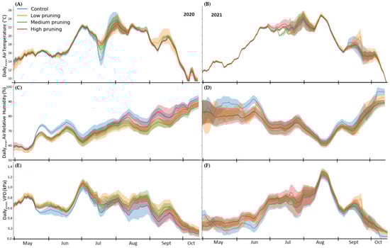
Figure 2.
Daily values of air temperature (A,B), relative air humidity (C,D), and vapor pressure deficit (VPD) (E,F)of the studied trees during the two growing seasons of 2020 and 2021. Solid lines represent daily mean values recorded by single TTs installed in the four replicates for each pruning treatment, while the shaded area around solid lines represents the standard deviation.
3.1. Sap Flow
Figure 3 and Figure 4 show the results of the sap flow of trees treated with different pruning intensities compared to the control trees (not pruned) in 2020 and 2021. High values indicate a greater amount of water transported by trees, which is potentially transpired. Considering the significance level α = 0.05, values of sap flow of medium and high pruning treatments are significantly lower than control throughout the whole first growing season (May–Sep 2020) except in October when the sap flow of all treatments is aligned, and the difference becomes non-significant. The difference in sap flow between the control and low pruning treatments was significant only in some periods during May and the first week of June, while it was non-significant during the rest of the 2020 growing season. The highest sap flow mean value for control trees was 55.38 L day−1, recorded during the 185th and the 191st day of the year (DOY) 2020, i.e., the first part of July 2020, when instead, the water transported by trees with medium and high pruning intensity was 37.80 (mean value) and 26.72 (mean value) L day−1, respectively. These peaks of sap flow correspond to higher air temperature and VPD (see Figure 1), which cause greater evapotranspiration, especially in trees with denser canopies (not pruned), as confirmed by many studies in the literature showing that vapor pressure deficit (VPD) is the key explanatory variable for sap flow for different plant species [68,109,110,111,112].
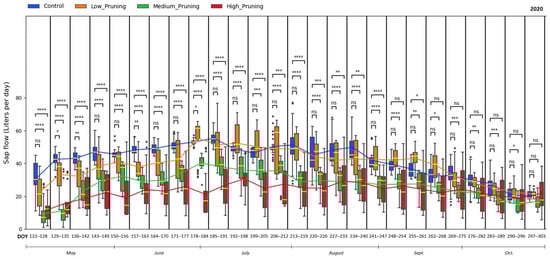
Figure 3.
Comparing the effect of pruning treatments (low, medium, and high) with respect to control (no pruning) on sap flow across the days of the year (DOY) during the vegetative cycle of 2020. Each box includes daily values in the range between the 25th and 75th percentiles of seven days of the four replications per treatment; whiskers extend to the 10th and 90th percentiles; and dots are outliers. The yellow line in each box represents the median value, while the continuous line joins the mean values of each box of the same treatment. The p-value of the Two-sided Mann-Whitney-Wilcoxon test is reported above the corresponding pair of boxplots, with ns (non-significant) when p ≥ 0.05; * when 0.01 < p ≤ 0.05; ** when 0.001 < p ≤ 0.01; *** when 0.0001 < p ≤ 0.001, **** when p ≤ 0.0001.
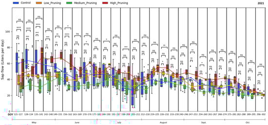
Figure 4.
Comparing the effect of pruning treatments (low, medium, and high) with respect to control (no pruning) on sap flow across the days of the year (DOY) during the vegetative cycle of 2021. Each box includes daily values in the range between the 25th and 75th percentiles of seven days of the four replications per treatment; whiskers extend to the 10th and 90th percentiles, and dots are outliers. The yellow line in each box represents the median value, while the continuous line joins the mean values of each box of the same treatment. The p-value of the Two-sided Mann−Whitney−Wilcoxon test is reported above the corresponding pair of boxplots, with ns (non-significant) when p ≥ 0.05; * when 0.01 < p ≤ 0.05; ** when 0.001 < p ≤ 0.01; *** when 0.0001 < p ≤ 0.001, **** when p ≤ 0.0001.
Results in terms of r-values of the Pearson correlation between sap flow and VPD (Table 2) show that VPD acts as the main driver of water transport in the plants for all treatments, both in the 2020 and 2021 growing years, with an average correlation equal to 0.73 during the two growing seasons. Similar correlations between sap flow and VPD have previously been reported for beech (0.85) in a beech-fir forest stand in the foothills of the Black Forest in Southwest Germany [110], and in other studies investigating jujube [112], apples [109], grapevines [113], pears (0.75) [68], and other tree species [111].
Table 2.
Pearson correlation coefficients (r-values) between sap flow and VPD during the two growing seasons assessed by comparing the average daily VPD and sap flow values for each treatment on the sample days.
Sap flow mean values observed in this study for not pruned trees varied between 42 and 55 L day−1 in July and August 2020, compared to 27–38 L day−1 and 24.5–27 L day−1 in trees treated with medium and high pruning, respectively, and dropped to 20.15 L day−1 in October with the senescence of the leaves, almost equal to the amount of water transpired by pruned trees. A similar trend for not pruned trees is observed by Magh et al. [110], who measured with the same thermal-based method a sap flow for European beech of 42, 74, and 19 L per day in May, July, and October, respectively. Instead, the reduction of sap flow in pruned trees compared to not pruned was similarly found in the literature, with some studies showing reduced transpiration by 12% in Eucalyptus [38] and 38% in wild cherry plantations [39] in the months just after the removal through pruning of vegetative parts of the tree, which has the direct effect of reducing the leaf area available for photosynthesis and transpiration [33,37,40].
According to the two-sided Mann−Whitney−Wilcoxon test, the difference between the control and all pruning treatments remained almost always non-significant throughout the whole 2021 growing season, with some exceptions for medium and high pruning during May and the beginning of June, with a mean value of sap flow ranging from 19 to 67 L day−1 for all trees. Interestingly, trees that went through high-intensity pruning showed high sap flow conductivity at the beginning of the second growing season (2021) compared to other treatments. A vigorous restart of the sap flow could be interpreted as a response in terms of vegetative growth of compensatory mechanisms to pruning, as also demonstrated by [114,115,116], who showed that after pruning, there is a mobilization of stored carbohydrates with changes in biomass allocation toward the tissue types that were lost, in this case, leaves and branches, with enhanced photosynthetic activity of the remaining leaves, ultimately posing a positive impact on carbon assimilation.
It is clear from these results that in the vegetative cycle of 2020, trees with more intense pruning require less water (21.4 L day−1 in July and 24.8 L day−1 in August) than control trees, which showed a greater amount of water transported with the highest mean value of about 55 L day−1 in July. At the end of the vegetative period (starting from September 2020), with the senescence of the leaves, the amount of water uptake by all treatments was aligned with the control. After one growing year, trees with different pruning intensities regained their potential and vigor to transport water across the stem equal to that of not pruned trees, with mean values of sap flow for all the trees that ranged between 27 and 67 L day−1 in May–August 2021 and no significant difference during the entire vegetative cycle 2021.
These findings clearly demonstrate that pruning treatment initially affects the sap flow, with a reduction in water use in the trees during the first months after woody removal, which, however, regains usual values at the end of the first growing season and completely realign during the following year. Studies in the literature, in fact, show that pruned trees mostly rebuilt their crowns after a year of development [115,117].
Interestingly, restrained water use as an effect of the pruning treatment could also be applied as a potential climate change adaptation strategy in chestnut forests devoted to fruit production, as already demonstrated in the literature for vineyards [118] and other crops [119]. In fact, the limited water requirement controlled by pruning during the dormancy period can strengthen the ability of chestnut trees to cope with intense drought periods during the growing season, which is expected to increase in frequency and length under future climate scenarios, especially in the Mediterranean region (IPCC, 2022).
3.2. Net Primary Productivity
Figure 5 and Figure 6 show the comparison of net primary productivity expressed as daily g of carbon absorbed per square meter of canopy by trees subject to different pruning intensities in 2020 and 2021. High values indicate a greater plant capacity to sequester carbon per unit of the crown surface. Considering α = 0.05, in the period May–June–July of the first growing season (2020) after pruning, values of NPP of low, medium, and high pruning treatments remained significantly lower than the control, while in August 2020, trees subjected to low pruning treatment increased their carbon sequestration capacity, and the difference became non-significant between low pruning treatment and control. In September–October 2020, the NPP of all pruning treatments aligned, and their differences were mostly non-significant when compared to the control. The highest daily mean NPP ranges between 5.5 and 5.7 g C day−1 per m2 of canopy were recorded for not pruned trees in July, compared to values between 3 and 4.5 g C day−1 per m2 of canopy in the same period for pruned trees. Then, NPP was reduced to the range of 0.16–1.12 g C day−1 per m2 of canopy at the end of the 2020 growing season for all the treatments.
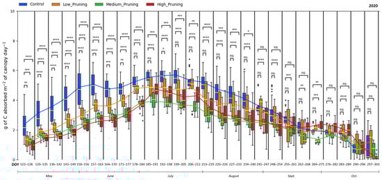
Figure 5.
Comparing the effect of pruning treatments (low, medium, and high) with respect to the control (no pruning) on carbon absorbed by the canopy across the days of the year (DOY) during the vegetative cycle of 2020. Each box includes daily values in the range between the 25th and 75th percentiles of seven days of the four replications per treatment; whiskers extend to the 10th and 90th percentiles, and dots are outliers. The yellow line in each box represents the median value, while the continuous line joins the mean values of each box of the same treatment. The p-value of the Two-sided Mann−Whitney−Wilcoxon test is reported above the corresponding pair of boxplots, with ns (non-significant) when p ≥ 0.05; * when 0.01 < p ≤ 0.05; ** when 0.001 < p ≤ 0.01; *** when 0.0001 < p ≤ 0.001, **** when p ≤ 0.0001.
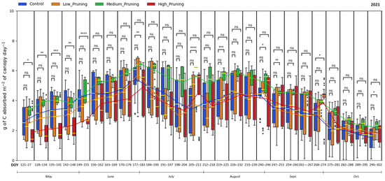
Figure 6.
Comparing the effect of pruning treatments (low, medium, and high) with respect to the control (no pruning) on carbon absorbed by the canopy across the days of the year (DOY) during the vegetative cycle of 2021. Each box includes daily values in the range between the 25th and 75th percentiles of seven days of the four replications per treatment; whiskers extend to the 10th and 90th percentiles; and dots are outliers. The yellow line in each box represents the median value, while the continuous line joins the mean values of each box of the same treatment. The p-value of the Two-sided Mann-Whitney-Wilcoxon test is reported above the corresponding pair of boxplots, with ns (non-significant) when p ≥ 0.05; * when 0.01 < p ≤ 0.05; ** when 0.001 < p ≤ 0.01; *** when 0.0001 < p ≤ 0.001, **** when p ≤ 0.0001.
The variability of NPP data is higher in 2021 compared to 2020, showing that the carbon sequestration potential of chestnut trees was not influenced by the intensity of pruning one year after the pruning treatment. In fact, the difference in NPP remained non-significant throughout the second growing season (2021), when the highest daily mean value of 6.34 g C day−1 per m2 of canopy was recorded in July. It is worth noting that trees not pruned, having maintained a denser canopy, show on average, a greater capacity to sequester carbon just after pruning; conversely, the trees with high intensity of pruning, having undergone a drastic reduction of the canopy, initially show a reduced capacity to sequester carbon, which they, however, recover starting in July/August, with the maximum growth of the canopy. Then, from mid-September and continuing in the subsequent vegetative year, all treatments align their NPP and show intense photosynthetic activity and thus a high carbon sequestration potential.
NPP values resulting in this study from the application of a LUE model based on APAR measured by the single TTs are in line with those reported in studies in the literature that modeled an NPP of 0.36 kg C m−2 yr−1 for chestnut stands in Tuscany region of Italy [120], 0.47 kg C m−2 yr−1 for Italian chestnut forests [121] and between 0.66 kg C m−2 yr−1 and 0.92 kg C m−2 yr−1 from 2000 to 2015 for the sweet chestnut in Iberian Peninsula [72]. In fact, the cumulative NPP measured in this study in the investigated chestnut forest is 0.68 kg C m−2 for the control trees and 0.56 kg C m−2, 0.44 kg C m−2, 0.47 kg C m−2 for the low, medium, and high-pruned trees, respectively, for the period from May to October 2020, and in the range between 0.60 and 0.84 kg C m−2 for all treatments in the period May-October 2021. These findings demonstrate that despite pruning affects productivity in the subsequent months, reducing in the short term up to 36% the NPP of medium-pruned trees compared to those not pruned, this management practice does not compromise the carbon sink capacity of chestnut trees, which although pruned remains in the range of the NPP expected in similar forests in the Mediterranean [72,120], particularly considering also that NPP values recorded in this study are referred not to the entire year but only to the months from May to October, which however are the ones during which the great part of the annual photosynthetic activity occurs. Moreover, one year after the pruning treatment, the NPP values of both pruned and not pruned trees equal the higher values in the range reported for similar forests in the Mediterranean [72,120], confirming that trees mostly rebuilt their crowns after a year of development [115,117].
The findings of this study demonstrate that the pruning treatment, while ensuring the recovery of chestnut trees for fruit production, initially entails a reduction in the carbon sink function of the chestnut forests in the months immediately after pruning. However, this initial disadvantage is rapidly and completely regained by the end of the first growing season, when the pruned trees show the same capacity as not pruned trees to remove and store carbon dioxide. Thus, this confirms the potential of forest and perennial woody land cover to provide multiple benefits both in terms of food and wood production as well as in terms of carbon sink and stock contributing to the climate change mitigation targets [122,123,124], as already demonstrated in some studies in the literature [114,116,125,126,127,128,129,130,131,132].
3.3. NDVI and Foliage Health
The NDVI, which expresses the canopy greenness index, clearly showed major differences due to the different canopy structures obtained under diverse pruning treatments (Figure 7). At the beginning of May 2020, trees that were subjected to low, medium, and high pruning showed NDVI values close to zero, meaning that trees were almost with no or few green leaves, compared to not pruned trees, showed in the same period mean NDVI value of 0.23 due to fact that they maintained a more extended canopy able to reach a high density of green leaves since the beginning of the spring growing period.
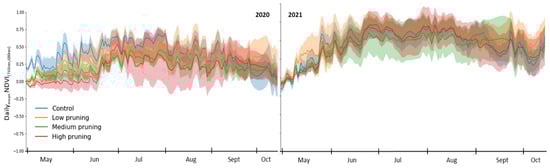
Figure 7.
Daily variation in NDVI of studied trees during the two growing seasons (2020–2021). Solid lines represent daily mean values recorded by single TTs installed in the four replicates for each pruning treatment, while shaded areas around solid lines represent standard deviation.
During May–June–July 2020, the NDVI of control (not pruned) trees was still significantly higher than that of medium- and high-pruned trees, indicating that control trees showed an obviously denser green coloration of the foliage. At the end of May 2020 not, pruned trees showed a daily mean NDVI value of 0.56, while highly pruned trees, having undergone a drastic reduction of the canopy, first showed a less green color of the canopy with a daily mean NDVI of 0.02 (absence/few leaves), which they however recovered starting from July-August 2020, with the maximum growth of the canopy. In fact, at the beginning of August 2020, the daily mean NDVI of the control, low, medium, and highly pruned trees were 0.7, 0.55, 0.43, and 0.27, respectively. As a deciduous tree species, chestnut starts senescence of the leaves with the onset of autumn, and accordingly, NDVI started decreasing toward lower values 0.1 recorded during October 2020 for all treatments.
What is interesting to note is that at the end of the first growing season (October 2020) and continuing to the second season (2021), the NDVI values of all the treatments aligned with each other with no significant difference between them, showing that the effect of pruning on the canopy is completely recovered at the end of the first vegetative cycle after pruning. In fact, in the second growing season (2021), although the change from spring to autumn was more evident, the difference between treatments was non-significant throughout the whole year. This confirms that pruned trees mostly rebuilt their crowns after a year of development, as has been widely demonstrated in the literature [115,117]. The NDVI curve from spring to autumn, representing a brown-green-brown canopy, was aligned with similar results observed using remote sensing for chestnut forests in Europe [133,134], although other spectral indexes, such as the Gitelson-Merzlyak chlorophyll index (R(NIR)/R700) or the green normalized difference vegetation index, could provide more refined results [135].
4. Conclusions
Pruning treatments applied to recover an abandoned chestnut forest in the Apennine of central Italy, besides allowing a combination of fruit production and ecosystem services provision, showed relevant effects on the trees’ ecophysiology, especially in the months just after the treatment. IoT sensors combined with Tree Talker devices were able to detect notable findings during the first growing season after pruning. These include a reduction in water use, especially in trees subjected to medium and high pruning treatments, along with a decrease in the carbon sink function, generally with no significant difference among the three tested pruning intensities. However, this study demonstrates and confirms that pruned trees regain the usual values of sap flow and carbon sink at the end of the first growing season and completely realign during the following year, showing that the effect of pruning on the canopy is completely recovered at the end of the first vegetative cycle after pruning, as also confirmed by NDVI values. As such, the initial disadvantage of carbon sequestration resulting from pruning treatments is swiftly remedied against the advantage of fostering the recovery of chestnut trees for fruit production. Furthermore, the controlled water requirements facilitated by pruning represent a potential climate change adaptation strategy for chestnut forests. This aspect strengthens the resilience of chestnut trees against prolonged and intensified drought periods during the growing season, which is projected to increase in frequency and duration under future climate scenarios, particularly in the Mediterranean region.
Author Contributions
Conceptualization, M.V.C. and R.V.; methodology, M.V.C., N.S. and R.V.; software, N.S.; validation, M.V.C., N.S. and G.V.; formal analysis, M.V.C. and N.S.; investigation, M.V.C. and N.S.; resources, M.V.C.; data curation, M.V.C. and N.S.; writing—original draft preparation, M.V.C. and N.S.; writing—review and editing, M.V.C., N.S., F.M., G.V., L.V.-A., I.M. and R.R.; visualization, M.V.C. and N.S.; supervision, M.V.C. and R.V.; project administration, I.M. and R.R.; funding acquisition, I.M. and R.R. All authors have read and agreed to the published version of the manuscript.
Funding
This research was funded by the Emilia Romagna regional program for rural development (PSR 2014-2020)—measure 16.1.01—Gruppi operativi del partenariato europeo per l’innovazione: “produttività e sostenitbilità dell’agricoltura”, Focus Area 5E—project n. 5111733 project “New techniques for monitoring the carbon balance and health status of wood and fruit chestnut forests-Talking Chestnuts”.
Data Availability Statement
Raw data supporting the conclusions of this article will be made available by the authors upon request.
Acknowledgments
The authors thank the Carisbo Foundation and the Italian Academy of Agriculture for allowing access to and data collection in the investigated chestnut forest.
Conflicts of Interest
The authors declare that this research was conducted in the absence of any commercial or financial relationships that could be construed as potential conflicts of interest. The funders had no role in the design of the study, collection, analyses, or interpretation of data, in the writing of the manuscript, or in the decision to publish the results.
References
- Conedera, M.; Tinner, W.; Krebs, P.; de Rigo, D.; Caudullo, G. Castanea Sativa in Europe: Distribution, Habitat, Usage and Threats. In European Atlas of Forest Tree Species; Publication Office of the European Union: Luxembourg, 2016; ISBN 978-92-79-36740-3. [Google Scholar]
- Míguez-Soto, B.; Fernández-Cruz, J.; Fernández-López, J. Mediterranean and Northern Iberian Gene Pools of Wild Castanea Sativa Mill. Are Two Differentiated Ecotypes Originated under Natural Divergent Selection. PLoS ONE 2019, 14, e0211315. [Google Scholar] [CrossRef]
- Roces-Díaz, J.; Diaz-Varela, E.; Anta, M.; Álvarez-Álvarez, P. Sweet Chestnut Agroforestry Systems in North-Western Spain: Classification, Spatial Distribution and an Ecosystem Services Assessment. For. Syst. 2018, 27, 10. [Google Scholar] [CrossRef]
- Jose, S. Agroforestry for Ecosystem Services and Environmental Benefits: An Overview. Agrofor. Syst. 2009, 76, 1–10. [Google Scholar] [CrossRef]
- Bombelli, A.; Di Paola, A.; Chiriacò, M.; Perugini, L.; Castaldi, S.; Valentini, R. Climate Change, Sustainable Agriculture and Food Systems: The World After the Paris Agreement. In Achieving the Sustainable Development Goals Through Sustainable Food Systems; Springer: Cham, Switzerland, 2019; pp. 25–34. ISBN 978-3-030-23968-8. [Google Scholar]
- Pezzi, G.; Maresi, G.; Conedera, M.; Ferrari, C. Woody species composition of chestnut stands in the Northern Apennines: The result of 200 years of changes in land use. Landsc. Ecol. 2011, 26, 1463–1476. [Google Scholar] [CrossRef]
- Gasparini, P.; Di Cosmo, L.; Floris, A.; Notarangelo, G.; Rizzo, M. INFC2015—Terzo Inventario Forestale Nazionale. In Consiglio per La Ricerca in Agricoltura e l’analisi Dell’economia Agraria, Unità Di Ricerca per Il Monitoraggio e La Pianificazione Forestale (CREA-MPF); Corpo Forestale delloStato, Ministero per le Politiche Agricole, Alimentari e Forestali: Rome, Italy, 2016; p. 341. [Google Scholar]
- Bruzzese, S.; Blanc, S.; Brun, F. Strategies for the Valorisation of Chestnut Resources in Italian Mountainous Areas from a Sustainable Development Perspective. Resources 2020, 9, 60. [Google Scholar] [CrossRef]
- Buonincontri, M.P.; Saracino, A.; Di Pasquale, G. The Transition of Chestnut (Castanea Sativa Miller) from Timber to Fruit Tree: Cultural and Economic Inferences in the Italian Peninsula. Holocene 2015, 25, 1111–1123. [Google Scholar] [CrossRef]
- Gullino, P.; Mellano, M.G.; Beccaro, G.; Devecchi, M.; Larcher, F. Land Strategies for the Management of Traditional Chestnut Landscapes in Pesio Valley, Italy: A Participatory Approach. Land 2020, 9, 536. [Google Scholar] [CrossRef]
- Murolo, S.; Bertoldi, D.; Pedrazzoli, F.; Mancini, M.; Romanazzi, G.; Maresi, G. New Symptoms in Castanea Sativa Stands in Italy: Chestnut Mosaic Virus and Nutrient Deficiency. Forests 2022, 13, 1894. [Google Scholar] [CrossRef]
- Chazdon, R.; Brancalion, P. Restoring Forests as a Means to Many Ends. Science 2019, 365, 24–25. [Google Scholar] [CrossRef]
- Di Paola, A.; Chiriacò, M.V.; Di Paola, F.; Nieddu, G. A Phenological Model for Olive (Olea europaea L. Var Europaea) Growing in Italy. Plants 2021, 10, 1115. [Google Scholar] [CrossRef]
- Conedera, M.; Manetti, M.; Giudici, F.; Amorini, E. Distribution and Economic Potential of the Sweet Chestnut (Castanea sativa Mill.) in Europe. Ecol. Mediterr. 2004, 30, 179–193. [Google Scholar] [CrossRef]
- Mura, R.; Vicentini, F.; Botti, L.M.; Chiriacò, M.V. Economic and Environmental Outcomes of a Sustainable and Circular Approach: Case Study of an Italian Wine-Producing Firm. J. Bus. Res. 2023, 154, 113300. [Google Scholar] [CrossRef]
- Beadle, C.; Barry, K.; Hardiyanto, E.; Irianto, R.; Junarto; Mohammed, C.; Rimbawanto, A. Effect of Pruning Acacia Mangium on Growth, Form and Heart Rot. For. Ecol. Manag. 2007, 238, 261–267. [Google Scholar] [CrossRef]
- Choi, S.T.; Park, D.S.; Hong, K.P.; Kang, S.M. Summer Pruning Effect on Tree Growth and Fruit Production of Persimmon. Adv. Hortic. Sci. 2013, 25, 164–169. [Google Scholar] [CrossRef]
- Freitas, T.R.; Santos, J.; Silva, A.; Fraga, H. Correction: Freitas et al. Influence of Climate Change on Chestnut Trees: A Review. Plants 2021, 10, 1463, Erratum in Plants 2022, 11, 1518. [Google Scholar]
- Colavolpe, M.B.; Fernando; Vaz Dias, F.; Serrazina, S.; Malhó, R.; Costa, R. Castanea Crenata Ginkbilobin-2-like Recombinant Protein Reveals Potential as an Antimicrobial against Phytophthora Cinnamomi, the Causal Agent of Ink Disease in European Chestnut. Forests 2023, 14, 785. [Google Scholar] [CrossRef]
- Rossi, M.; De Feudis, M.; Trenti, W.; Gherardi, M.; Vianello, G.; Vittori Antisari, L. GIS-Based Geopedological Approach for Assessing Land Suitability for Chestnut (Castanea sativa Mill.) Groves for Fruit Production. Forests 2023, 14, 224. [Google Scholar] [CrossRef]
- Pires, A.L.; Portela, E. Impact of Management Practices on Chestnut Grove Nutrient Budgets. Acta Hortic. 2005, 693, 677–684. [Google Scholar] [CrossRef]
- Venanzi, R.; Picchio, R.; Grigolato, S.; Spinelli, R. Soil Disturbance Induced by Silvicultural Treatment in Chestnut (Castanea sativa Mill.) Coppice and Post-Disturbance Recovery. Forests 2020, 11, 1053. [Google Scholar] [CrossRef]
- Massantini, R.; Moscetti, R.; Frangipane, M.T. Evaluating Progress of Chestnut Quality: A Review of Recent Developments. Trends Food Sci. Technol. 2021, 113, 245–254. [Google Scholar] [CrossRef]
- Amorini, E.; Bruschini, S.; Manetti, M.C. Alternative Silvicultural Systems in Chestnut (Castanea sativa Mill.) Coppice: Effects of Silvicultural Practices on Stand Structure and Tree Growth. Ecol. Mediterr. 2000, 26, 155–162. [Google Scholar] [CrossRef]
- Manetti, M.; Conedera, M.; Pelleri, F.; Montini, P.; Maltoni, A.; Mariotti, B.; Pividori, M.; Marcolin, E. Optimizing Quality Wood Production in Chestnut (Castanea sativa Mill.) Coppices. For. Ecol. Manag. 2022, 523, 120490. [Google Scholar] [CrossRef]
- Maltoni, A.; Mariotti, B.; Jacobs, D.; Tani, A. Pruning Methods to Restore Castanea sativa Stands Attacked by Dryocosmus Kuriphilus. New For. 2012, 43, 869–885. [Google Scholar] [CrossRef]
- Mariotti, B.; Castellotti, T.; Conedera, M.; Corona, P.; Manetti, M.C.; Romano, R.; Tani, A.; Maltoni, A. Linee Guida per La Gestione Selvicolturale Dei Castagneti Da Frutto. In Rete Rurale Nazionale 2014–2020, Scheda n. 22.2; Foreste, Consiglio per la ricerca in agricoltura e l’analisi dell’economia agraria: Roma, Italy, 2019. [Google Scholar]
- Ebone, A.; Terzuolo, P.G.; Boni, I.; Brenta, P.; Palenzona, M.; Ferrara, A.M. Castagneti Da Frutto in Piemonte Pubblicazione Realizzata Nel 2020 Nell’ambito Della Collana “Le Guide Selvicolturali” Della Regione Piemonte. Available online: https://www.regione.piemonte.it/web/sites/default/files/media/documenti/2021-05/guida_castagno_030521_bq_0.pdf (accessed on 30 August 2024).
- De Feudis, M.; Falsone, G.; Vianello, G.; Vittori Antisari, L. The Conversion of Abandoned Chestnut Forests to Managed Ones Does Not Affect the Soil Chemical Properties and Improves the Soil Microbial Biomass Activity. Forests 2020, 11, 786. [Google Scholar] [CrossRef]
- De Feudis, M.; Vianello, G.; Vittori Antisari, L. Soil Organic Carbon Stock Assessment for Volunteer Carbon Removal Benefit: Methodological Approach in Chestnut Orchard for Fruit Production. Environments 2023, 10, 83. [Google Scholar] [CrossRef]
- Kumar, M.; Rawat, V.; Rawat, J.M.S.; Tomar, Y.K. Effect of Pruning Intensity on Peach Yield and Fruit Quality. Sci. Hortic. 2010, 125, 218–221. [Google Scholar] [CrossRef]
- Springmann, S.; Rogers, R.; Spiecker, H. Impact of Artificial Pruning on Growth and Secondary Shoot Development of Wild Cherry (Prunus avium L.). For. Ecol. Manag. 2011, 261, 764–769. [Google Scholar] [CrossRef]
- Asrey, R.; Patel, V.B.; Barman, K.; Pal, R.K. Pruning Affects Fruit Yield and Postharvest Quality in Mango (Mangifera indica L.) Cv. Amrapali. Fruits 2013, 68, 367–380. [Google Scholar] [CrossRef]
- Leiva-Rojas, E.I.; Gutiérrez-Brito, E.E.; Pardo-Macea, C.J.; Ramírez-Pisco, R. Vegetative and Reproductive Behavior of Cocoa (Theobroma cacao L.) Due to Pruning|Comportamiento Vegetativo y Reproductivo Del Cacao (Theobroma cacao L.) Por Efecto de La Poda. Rev. Fitotec. Mex. 2019, 42, 137–146. [Google Scholar] [CrossRef]
- Bandara, G.D.; Whitehead, D.; Mead, D.; Moot, D. Effects of Pruning and Understorey Vegetation on Crown Development, Biomass Increment and above-Ground Carbon Partitioning in Pinus Radiata D. Don Trees Growing at a Dryland Agroforestry Site. For. Ecol. Manag. 1999, 124, 241–254. [Google Scholar] [CrossRef]
- Pinkard, E.; Battaglia, M.; Beadle, C.; Sands, P. Modeling the Effect of Physiological Responses to Green Pruning on Net Biomass Production of Eucalyptus nitens. Tree Physiol. 1999, 19, 1–12. [Google Scholar] [CrossRef]
- Buyinza, J.; Muthuri, C.; Denton, M.; Nuberg, I. Impact of Tree Pruning on Water Use in Tree-Coffee Systems on Smallholder Farms in Eastern Uganda. Agrofor. Syst. 2023, 97, 953–964. [Google Scholar] [CrossRef]
- Forrester, D.; Collopy, J.; Beadle, C.; Warren, C.; Baker, T. Effect of Thinning, Pruning and Nitrogen Fertiliser Application on Transpiration, Photosynthesis and Water-Use Efficiency in a Young Eucalyptus nitens Plantation. For. Ecol. Manag. 2012, 266, 286–300. [Google Scholar] [CrossRef]
- Molina, A.J.; Aranda, X.; Llorens, P.; Galindo, A.; Biel, C. Sap Flow of a Wild Cherry Tree Plantation Growing under Mediterranean Conditions: Assessing the Role of Environmental Conditions on Canopy Conductance and the Effect of Branch Pruning on Water Productivity. Agric. Water Manag. 2019, 218, 222–233. [Google Scholar] [CrossRef]
- Suchocka, M.; Swoczyna, T.; Kosno-Jończy, J.; Kalaji, H.M. Impact of Heavy Pruning on Development and Photosynthesis of Tilia Cordata Mill. Trees. PLoS ONE 2021, 16, e0256465. [Google Scholar] [CrossRef] [PubMed]
- Niccoli, F.; Pacheco-Solana, A.; Delzon, S.; Kabala, J.P.; Asgharinia, S.; Castaldi, S.; Valentini, R.; Battipaglia, G. Effects of Wildfire on Growth, Transpiration and Hydraulic Properties of Pinus Pinaster Aiton Forest. Dendrochronologia 2023, 79, 126086. [Google Scholar] [CrossRef]
- Asgharinia, S.; Leberecht, M.; Belelli Marchesini, L.; Frieß, N.; Gianelle, D.; Nauss, T.; Opgenoorth, L.; Yates, J.; Valentini, R. Towards Continuous Stem Water Content and Sap Flux Density Monitoring: IoT-Based Solution for Detecting Changes in Stem Water Dynamics. Forests 2022, 13, 1040. [Google Scholar] [CrossRef]
- IUSS Working Group WRB. World Reference Base for Soil Resources 2014; World Soil Resources Reports No. 106; Schad, P., van Huyssteen, C., Micheli, E., Eds.; FAO: Rome, Italy, 2014; p. 189. ISBN 978-92-5-108369-7. [Google Scholar]
- Thurner, M.; Beer, C.; Crowther, T.; Falster, D.; Manzoni, S.; Prokushkin, A.; Schulze, E. Sapwood Biomass Carbon in Northern Boreal and Temperate Forests. Glob. Ecol. Biogeogr. 2019, 28, 640–660. [Google Scholar] [CrossRef]
- Matasov, V.; Belelli Marchesini, L.; Yaroslavtsev, A.; Sala, G.; Fareeva, O.; Seregin, I.; Castaldi, S.; Vasenev, V.; Valentini, R. IoT Monitoring of Urban Tree Ecosystem Services: Possibilities and Challenges. Forests 2020, 11, 775. [Google Scholar] [CrossRef]
- Valentini, R.; Belelli Marchesini, L.; Sala, G.; Yaroslavtsev, A.; Vasenev, V.; Castaldi, S. New Tree Monitoring Systems: From Industry 4.0 to Nature 4.0. Ann. Silvic. Res. 2019, 43, 84–88. [Google Scholar] [CrossRef]
- Do, F.; Puangjumpa, N.; Rocheteau, A.; Duthoit, M.; Nhean, S.; Ayutthaya, S. Towards Reduced Heating Duration in the Transient Thermal Dissipation System of Sap Flow Measurements. Acta Hortic. 2018, 1222, 149–154. [Google Scholar] [CrossRef]
- Granier, A. Evaluation of Transpiration in a Douglas-Fir Stand by Means of Sap Flow Measurements. Tree Physiol. 1987, 3, 309–320. [Google Scholar] [CrossRef] [PubMed]
- Gimenez, C.; Gallardo, M.; Thompson, R.B. Plant–Water Relations. In Encyclopedia of Soils in the Environment; Elsevier: Amsterdam, Netherlands, 2013; pp. 231–238. ISBN 978-0-12-409548-9. [Google Scholar]
- Lagergren, F.; Lindroth, A. Variation in Sapflow and Stem Growth in Relation to Tree Size, Competition and Thinning in a Mixed Forest of Pine and Spruce in Sweden. For. Ecol. Manag. 2004, 188, 51–63. [Google Scholar] [CrossRef]
- Lagergren, F.; Lindroth, A. Transpiration Response to Soil Moisture in Pine and Spruce Trees in Sweden. Agric. For. Meteorol. 2002, 112, 67–85. [Google Scholar] [CrossRef]
- Swanson, R.H. Significant Historical Developments in Thermal Methods for Measuring Sap Flow in Trees. Agric. For. Meteorol. 1994, 72, 113–132. [Google Scholar] [CrossRef]
- Tu, J.; Wei, X.; Huang, B.; Fan, H.; Jian, M.; Li, W. Improvement of Sap Flow Estimation by Including Phenological Index and Time-Lag Effect in Back-Propagation Neural Network Models. Agric. For. Meteorol. 2019, 276–277, 107608. [Google Scholar] [CrossRef]
- Flo, V.; Martinez-Vilalta, J.; Steppe, K.; Schuldt, B.; Poyatos, R. A Synthesis of Bias and Uncertainty in Sap Flow Methods. Agric. For. Meteorol. 2019, 271, 362–374. [Google Scholar] [CrossRef]
- Liu, J.; Li, D.; Fernández, J.E.; Coleman, M.; Hu, W.; Di, N.; Zou, S.; Liu, Y.; Xi, B.; Clothier, B. Variations in Water-Balance Components and Carbon Stocks in Poplar Plantations with Differing Water Inputs over a Whole Rotation: Implications for Sustainable Forest Management under Climate Change. Agric. For. Meteorol. 2022, 320, 108958. [Google Scholar] [CrossRef]
- Zhao, X.; Li, X.; Hu, W.; Liu, J.; Di, N.; Duan, J.; Li, D.; Liu, Y.; Guo, Y.; Wang, A.; et al. Long-Term Variation of the Sap Flow to Tree Diameter Relation in a Temperate Poplar Forest. J. Hydrol. 2023, 618, 129189. [Google Scholar] [CrossRef]
- Wullschleger, S.; King, A. Radial Variation in Sap Velocity as a Function of Stem Diameter and Sapwood Thickness in Yellow-Poplar Trees. Tree Physiol. 2000, 20, 511–518. [Google Scholar] [CrossRef]
- Cohen, Y.; Cohen, S.; Cantuarias-Aviles, T.; Schiller, G. Variations in the Radial Gradient of Sap Velocity in Trunks of Forest and Fruit Trees. Plant Soil 2008, 305, 49–59. [Google Scholar] [CrossRef]
- Looker, N.; Martin, J.; Jencso, K.; Hu, J. Contribution of Sapwood Traits to Uncertainty in Conifer Sap Flow as Estimated with the Heat-Ratio Method. Agric. For. Meteorol. 2016, 223, 60–71. [Google Scholar] [CrossRef]
- Poyatos, R.; Martinez Vilalta, J.; Cermák, J.; Ceulemans, R.; Granier, A.; Irvine, J.; Köstner, B.; Lagergren, F.; Meiresonne, L.; Nadezhdina, N.; et al. Plasticity in Hydraulic Architecture of Scots Pine across Eurasia. Oecologia 2007, 153, 245–259. [Google Scholar] [CrossRef]
- Santiago, L.S.; Goldstein, G.; Meinzer, F.C.; Fownes, J.H.; Mueller-Dombois, D. Transpiration and Forest Structure in Relation to Soil Waterlogging in a Hawaiian Montane Cloud Forest. Tree Physiol. 2000, 20, 673–681. [Google Scholar] [CrossRef] [PubMed][Green Version]
- Oren, R.; Pataki, D.E. Transpiration in Response to Variation in Microclimate and Soil Moisture in Southeastern Deciduous Forests. Oecologia 2001, 127, 549–559. [Google Scholar] [CrossRef] [PubMed]
- de Blécourt, M.; Gröngröft, A.; Thomsen, S.; Eschenbach, A. Temporal Variation and Controlling Factors of Tree Water Consumption in the Thornbush Savanna. J. Arid Environ. 2021, 189, 104500. [Google Scholar] [CrossRef]
- Chen, X.; Li, Y.; Li, Y.; Li, W.; Du, Q.; Lou, J.; Li, P.; Zhang, D. A Plasma Membrane Aquaporin Is Potentially Involved in Moderating Water Stress and Photosynthetic Depression by Sustaining Water Transport and CO2 Uptake under High VPD Stress Conditions in Solanum lycopersicum (Tomato). Sci. Hortic. 2022, 301, 111128. [Google Scholar] [CrossRef]
- Jiao, L.; Lu, N.; Sun, G.; Ward, E.J.; Fu, B. Biophysical Controls on Canopy Transpiration in a Black Locust (Robinia Pseudoacacia) Plantation on the Semi-Arid Loess Plateau, China. Ecohydrology 2016, 9, 1068–1081. [Google Scholar] [CrossRef]
- Wang, W.J.; He, H.S.; Thompson, F.R.; Fraser, J.S.; Dijak, W.D. Changes in Forest Biomass and Tree Species Distribution under Climate Change in the Northeastern United States. Landsc. Ecol. 2017, 32, 1399–1413. [Google Scholar] [CrossRef]
- Jung, E.Y.; Otieno, D.; Lee, B.; Lim, J.H.; Kang, S.K.; Schmidt, M.W.T.; Tenhunen, J. Up-Scaling to Stand Transpiration of an Asian Temperate Mixed-Deciduous Forest from Single Tree Sapflow Measurements. Plant Ecol. 2011, 212, 383–395. [Google Scholar] [CrossRef]
- Fan, B.; Liu, Z.; Xiong, K.; Li, Y.; Li, K.; Yu, X. Influence of Environmental Factors on the Sap Flow Activity of the Golden Pear in the Growth Period of Karst Area in Southern China. Water 2022, 14, 1707. [Google Scholar] [CrossRef]
- Fan, J.-W.; Shao, Q.-Q.; Liu, J.-Y.; Wang, J.-B.; Harris, W.; Chen, Z.-Q.; Zhong, H.-P.; Xu, X.-L.; Liu, R.-G. Assessment of Effects of Climate Change and Grazing Activity on Grassland Yield in the Three Rivers Headwaters Region of Qinghai–Tibet Plateau, China. Environ. Monit. Assess. 2010, 170, 571–584. [Google Scholar] [CrossRef] [PubMed]
- Xue, S.; Ma, B.; Wang, C.; Li, Z. Identifying Key Landscape Pattern Indices Influencing the NPP: A Case Study of the Upper and Middle Reaches of the Yellow River. Ecol. Model. 2023, 484, 110457. [Google Scholar] [CrossRef]
- Yu, R. An Improved Estimation of Net Primary Productivity of Grassland in the Qinghai-Tibet Region Using Light Use Efficiency with Vegetation Photosynthesis Model. Ecol. Model. 2020, 431, 109121. [Google Scholar] [CrossRef]
- Pérez-Girón, J.C.; Álvarez-Álvarez, P.; Díaz-Varela, E.R.; Mendes Lopes, D.M. Influence of Climate Variations on Primary Production Indicators and on the Resilience of Forest Ecosystems in a Future Scenario of Climate Change: Application to Sweet Chestnut Agroforestry Systems in the Iberian Peninsula. Ecol. Indic. 2020, 113, 106199. [Google Scholar] [CrossRef]
- Gulbeyaz, O.; Bond-Lamberty, B.; Akyürek, Z.; West, T. A New Approach to Evaluate the MODIS Annual NPP Product (MOD17A3) Using Forest Field Data from Turkey. Int. J. Remote Sens. 2018, 39, 2560–2578. [Google Scholar] [CrossRef]
- Huang, N.; Niu, Z.; Wu, C.; Tappert, M.C. Modeling Net Primary Production of a Fast-Growing Forest Using a Light Use Efficiency Model. Ecol. Model. 2010, 221, 2938–2948. [Google Scholar] [CrossRef]
- Huang, L.; Ning, Z.; Zhang, X. Impacts of Caterpillar Disturbance on Forest Net Primary Production Estimation in China. Ecol. Indic. 2010, 10, 1144–1151. [Google Scholar] [CrossRef]
- Yu, D.; Shi, P.; Shao, H.; Zhu, W.; Pan, Y. Modelling Net Primary Productivity of Terrestrial Ecosystem in East Asia Region Based on Improved CASA Ecosystem Model. Int. J. Remote Sens. 2009, 30, 4851–4866. [Google Scholar] [CrossRef]
- Zhou, B.; Liao, Z.; Chen, S.; Jia, H.; Zhu, J.; Fei, X.-H. Net Primary Productivity of Forest Ecosystems in the Southwest Karst Region from the Perspective of Carbon Neutralization. Forests 2022, 13, 1367. [Google Scholar] [CrossRef]
- Monteith, J.L. Solar Radiation and Productivity in Tropical Ecosystems. J. Appl. Ecol. 1972, 9, 747–766. [Google Scholar] [CrossRef]
- Zarei, A.; Chemura, A.; Gleixner, S.; Hoff, H. Evaluating the Grassland NPP Dynamics in Response to Climate Change in Tanzania. Ecol. Indic. 2021, 125, 107600. [Google Scholar] [CrossRef]
- Running, S.W.; Nemani, R.R.; Heinsch, F.A.; Zhao, M.; Reeves, M.; Hashimoto, H. A Continuous Satellite-Derived Measure of Global Terrestrial Primary Production. BioScience 2004, 54, 547–560. [Google Scholar] [CrossRef]
- Landsberg, J.J. Physiological Ecology of Forest Production; Applied botany and crop science; Academic Press: Cambridge, MA, USA, 1986; ISBN 978-0-12-435965-9. [Google Scholar]
- Gower, S.T.; Kucharik, C.J.; Norman, J.M. Direct and Indirect Estimation of Leaf Area Index, fAPAR, and Net Primary Production of Terrestrial Ecosystems. Remote Sens. Environ. 1999, 70, 29–51. [Google Scholar] [CrossRef]
- Doughty, C.; Asner, G.; Martin, R. Predicting Tropical Plant Physiology from Leaf and Canopy Spectroscopy. Oecologia 2010, 165, 289–299. [Google Scholar] [CrossRef]
- Ollinger, S.V. Sources of Variability in Canopy Reflectance and the Convergent Properties of Plants. New Phytol. 2011, 189, 375–394. [Google Scholar] [CrossRef]
- Federici, S.; Vitullo, M.; Tulipano, S.; De Lauretis, R.; Seufert, G. An Approach to Estimate Carbon Stocks Change in Forest Carbon Pools under the UNFCCC: The Italian Case. IForest Biogeosciences For. 2008, 1, 85–95. [Google Scholar] [CrossRef]
- Asner, G.; Martin, R.; Carlson, K.; Vitousek, P. Vegetation–Climate Interactions among Native and Invasive Species in Hawaiian Rainforest. Ecosystems 2006, 9, 1106–1117. [Google Scholar] [CrossRef]
- Beyer, M.; Ahmad, R.; Yang, B.; Rodríguez-Bocca, P. Deep Spatial-Temporal Graph Modeling for Efficient NDVI Forecasting. Smart Agric. Technol. 2023, 4, 100172. [Google Scholar] [CrossRef]
- Fokeng, R.M.; Fogwe, Z.N. Landsat NDVI-Based Vegetation Degradation Dynamics and Its Response to Rainfall Variability and Anthropogenic Stressors in Southern Bui Plateau, Cameroon. Geosystems Geoenvironment 2022, 1, 100075. [Google Scholar] [CrossRef]
- Hovi, A.; Forsström, P.; Mõttus, M.; Rautiainen, M. Evaluation of Accuracy and Practical Applicability of Methods for Measuring Leaf Reflectance and Transmittance Spectra. Remote Sens. 2017, 10, 25. [Google Scholar] [CrossRef]
- De La Iglesia Martinez, A.; Labib, S.M. Demystifying Normalized Difference Vegetation Index (NDVI) for Greenness Exposure Assessments and Policy Interventions in Urban Greening. Environ. Res. 2023, 220, 115155. [Google Scholar] [CrossRef] [PubMed]
- Du, J.; Quan, Z.; Fang, S.; Liu, C.; Wu, J.; Fu, Q. Spatiotemporal Changes in Vegetation Coverage and Its Causes in China since the Chinese Economic Reform. Environ. Sci. Pollut. Res. 2020, 27, 1144–1159. [Google Scholar] [CrossRef]
- Evans, K.L.; James, N.A.; Gaston, K.J. Abundance, Species Richness and Energy Availability in the North American Avifauna. Glob. Ecol. Biogeogr. 2006, 15, 372–385. [Google Scholar] [CrossRef]
- Guan, J.; Yao, J.; Li, M.; Zheng, J. Assessing the Spatiotemporal Evolution of Anthropogenic Impacts on Remotely Sensed Vegetation Dynamics in Xinjiang, China. Remote Sens. 2021, 13, 4651. [Google Scholar] [CrossRef]
- Lamchin, M.; Lee, W.-K.; Jeon, S.W.; Wang, S.W.; Lim, C.H.; Song, C.; Sung, M. Long-Term Trend and Correlation between Vegetation Greenness and Climate Variables in Asia Based on Satellite Data. Sci. Total Environ. 2018, 618, 1089–1095. [Google Scholar] [CrossRef]
- Xiao, J.; Moody, A. Trends in Vegetation Activity and Their Climatic Correlates: China 1982 to 1998. Int. J. Remote Sens. 2004, 25, 5669–5689. [Google Scholar] [CrossRef]
- Al-Abbas, A.H.; Barr, R.; Hall, J.D.; Crane, F.L.; Baumgardner, M.F. Spectra of Normal and Nutrient-Deficient Maize Leaves1. Agron. J. 1974, 66, 16–20. [Google Scholar] [CrossRef]
- Smithson, P.A. Microclimatic Landscape Design: Creating Thermal Comfort and Energy Efficiency. Int. J. Climatol. 1997, 17, 225–226. [Google Scholar] [CrossRef]
- Woolley, J.T. Reflectance and Transmittance of Light by Leaves. Plant Physiol. 1971, 47, 656–662. [Google Scholar] [CrossRef]
- Baranoski, G.; Rokne, J. An Algorithmic Reflectance and Transmittance Model for Plant Tissue. Comput. Graph. Forum 1997, 16, C141–C150. [Google Scholar] [CrossRef]
- Baranoski, G.; Rokne, J. Efficiently Simulating Scattering of Light by Leaves. Vis. Comput. 2001, 17, 491–505. [Google Scholar] [CrossRef]
- Brakke, T.; Smith, J.; Harnden, J. Bidirectional Scattering of Light from Tree Leaves. Remote Sens. Environ. 1989, 29, 175–183. [Google Scholar] [CrossRef]
- Hovi, A.; Raitio, P.; Rautiainen, M. A Spectral Analysis of 25 Boreal Tree Species. Silva Fenn. 2017, 51. [Google Scholar] [CrossRef]
- Minelli, A.; Gaetani, M.; Grossi, N.; Magni, S.; Caturegli, L. Reflectance, Absorbance and Transmittance Spectra of Bermudagrass and Manilagrass Turfgrass Canopies. PLoS ONE 2017, 12, e0188080. [Google Scholar] [CrossRef]
- Jenkins, J.P.; Richardson, A.; Braswell, B.; Ollinger, S.V.; Hollinger, D.; Smith, M.-L. Refining Light-Use Efficiency Calculations for a Deciduous Forest Canopy Using Simultaneous Tower-Based Carbon Flux and Radiometric Measurements. Agric. For. Meteorol. 2007, 143, 64–79. [Google Scholar] [CrossRef]
- Nagler, P.; Glenn, E.; Thompson, T.; Huete, A. Leaf Area Index and Normalized Difference Vegetation Index as Predictors of Canopy Characteristics and Light Interception by Riparian Species on the Lower Colorado River. Agric. For. Meteorol. 2004, 125, 1–17. [Google Scholar] [CrossRef]
- Chen, J.-J.; Zhen, S.; Sun, Y. Estimating Leaf Chlorophyll Content of Buffaloberry Using Normalized Difference Vegetation Index Sensors. HortTechnology 2021, 31, 297–303. [Google Scholar] [CrossRef]
- Dworak, V.; Selbeck, J.; Dammer, K.-H.; Hoffmann, M.; Zarezadeh, A.; Bobda, C. Strategy for the Development of a Smart NDVI Camera System for Outdoor Plant Detection and Agricultural Embedded Systems. Sensors 2013, 13, 1523–1538. [Google Scholar] [CrossRef]
- Pereira, M.; Caramelo, L.; Gouveia, C.; Gomes-Laranjo, J.; Magalhães, M. Assessment of Weather-Related Risk on Chestnut Productivity. Nat. Hazards Earth Syst. Sci. 2011, 11, 2729–2739. [Google Scholar] [CrossRef]
- Liu, C.; Du, T.; Li, F.; Kang, S.; Li, S.; Tong, L. Trunk Sap Flow Characteristics during Two Growth Stages of Apple Tree and Its Relationships with Affecting Factors in an Arid Region of Northwest China. Agric. Water Manag. 2012, 104, 193–202. [Google Scholar] [CrossRef]
- Magh, R.-K.; Bonn, B.; Grote, R.; Burzlaff, T.; Pfautsch, S. Rennenberg Drought Superimposes the Positive Effect of Silver Fir on Water Relations of European Beech in Mature Forest Stands. Forests 2019, 10, 897. [Google Scholar] [CrossRef]
- Sun, X.; Li, J.; Cameron, D.; Moore, G. On the Use of Sap Flow Measurements to Assess the Water Requirements of Three Australian Native Tree Species. Agronomy 2021, 12, 52. [Google Scholar] [CrossRef]
- Xinguang, W.; Bo, L.; Chengjiu, G.; Youke, W.; He, J.; Liu, S.; Tieliang, W.; Mingze, Y. Identification of Sap Flow Driving Factors of Jujube Plantation in Semi-Arid Areas in Northwest China. Int. J. Agric. Biol. Eng. 2017, 10, 173–184. [Google Scholar] [CrossRef]
- Baert, A.; Villez, K.; Kathy, S. Automatic Drought Stress Detection in Grapevines without Using Conventional Threshold Values. Plant Soil 2013, 369, 439–452. [Google Scholar] [CrossRef]
- Anten, N.; Martinez-Ramos, M.; Ackerly, D. Defoliation and Growth in an Understory Palm: Quantifying the Contributions of Compensatory Responses. Ecology 2003, 84, 2905–2918. [Google Scholar] [CrossRef]
- Tosto, A.; Zuidema, P.A.; Goudsmit, E.; Evers, J.B.; Anten, N.P.R. The Effect of Pruning on Yield of Cocoa Trees Is Mediated by Tree Size and Tree Competition. Sci. Hortic. 2022, 304, 111275. [Google Scholar] [CrossRef]
- Trumble, J.T.; Kolodny-Hirsch, D.M.; Ting, I.P. Plant Compensation for Arthropod Herbivory. Annu. Rev. Entomol. 1993, 38, 93–119. [Google Scholar] [CrossRef]
- Zeng, B. Aboveground Biomass Partitioning and Leaf Development of Chinese Subtropical Trees Following Pruning. For. Ecol. Manag. 2003, 173, 135–144. [Google Scholar] [CrossRef]
- Schäfer, J.; Friedel, M.; Molitor, D.; Stoll, M. Semi-Minimal-Pruned Hedge (SMPH) as a Climate Change Adaptation Strategy: Impact of Different Yield Regulation Approaches on Vegetative and Generative Development, Maturity Progress and Grape Quality in Riesling. Appl. Sci. 2021, 11, 3304. [Google Scholar] [CrossRef]
- Ma, L.; Wang, X.; Gao, Z.; Youke, W.; Nie, Z.; Liu, X. Canopy Pruning as a Strategy for Saving Water in a Dry Land Jujube Plantation in a Loess Hilly Region of China. Agric. Water Manag. 2019, 216, 436–443. [Google Scholar] [CrossRef]
- Chiesi, M.; Moriondo, M.; Maselli, F.; Gardin, L.; Fibbi, L.; Bindi, M.; Running, S.W. Simulation of Mediterranean Forest Carbon Pools under Expected Environmental Scenarios. Can. J. For. Res. 2010, 40, 850–860. [Google Scholar] [CrossRef]
- Nolè, A.; Collalti, A.; Borghetti, M.; Chiesi, M.; Chirici, G.; Magnani, F.; Valentini, R. The role of managed forest ecosystems: A modeling based approach. In The Greenhouse Gas Balance of Italy: An Insight on Managed and Natural Terrestrial Ecosystems; Springer: Berlin/Heidelberg, Germany, 2014; pp. 71–85. [Google Scholar]
- Kay, S.; Rega, C.; Moreno, G.; den Herder, M.; Palma, J.H.; Borek, R.; Herzog, F. Agroforestry creates carbon sinks whilst enhancing the environment in agricultural landscapes in Europe. Land Use Policy 2019, 83, 581–593. [Google Scholar] [CrossRef]
- Di Lallo, G.; Chiriacò, M.V.; Tarasova, E.; Köhl, M.; Perugini, L. The Land Sector in the Low Carbon Emission Strategies in the European Union: Role and Future Expectations. Clim. Policy 2024, 24, 586–600. [Google Scholar] [CrossRef]
- Russell, A.E.; Kumar, B.M. Forestry for a low-carbon future: Integrating forests and wood products into climate change strategies. Environ. Sci. Policy Sustain. Dev. 2017, 59, 16–23. [Google Scholar] [CrossRef]
- Cirigliano, P.; Chiriacò, M.V.; Nunez, A.; Dal Monte, G.; Labagnara, T. Efecto Combinado de La Aplicación de Riego y Compost Sobre La Composición de La Baya Montepulciano En Un Entorno Volcánico de La Región de Lacio (Italia Central). Cienc. E Investig. Agrar. 2017, 44, 195–206. [Google Scholar] [CrossRef]
- Arodudu, O.; Therasme, O.; Volk, T.; Malmsheimer, R.; Crovella, P.; Germain, R.; Kloster, D.; Kumar, D. Towards a Carbon Accounting Framework for Assessing the Benefits of Biogenic Wood Carbon to Net Zero Carbon Targets. Forests 2023, 14, 1959. [Google Scholar] [CrossRef]
- Ganatsas, P.; Tsakaldimi, M.; Petaloudi, L.-M. Factors Affecting Long-Term Soil Organic Carbon Storage in Greek Forests. Forests 2023, 14, 1518. [Google Scholar] [CrossRef]
- Hammad, H.M.; Fasihuddin Nauman, H.M.; Abbas, F.; Ahmad, A.; Bakhat, H.F.; Saeed, S.; Shah, G.M.; Ahmad, A.; Cerdà, A. Carbon Sequestration Potential and Soil Characteristics of Various Land Use Systems in Arid Region. J. Environ. Manag. 2020, 264, 110254. [Google Scholar] [CrossRef]
- Menéndez-Miguélez, M.; Álvarez-Álvarez, P.; Pardos, M.; Madrigal, G.; Ruiz-Peinado, R.; López-Senespleda, E.; Del Río, M.; Calama, R. Development of Tools to Estimate the Contribution of Young Sweet Chestnut Plantations to Climate-Change Mitigation. For. Ecol. Manag. 2023, 530, 120761. [Google Scholar] [CrossRef]
- Sahoo, U.K.; Nath, A.J.; Lalnunpuii, K. Biomass Estimation Models, Biomass Storage and Ecosystem Carbon Stock in Sweet Orange Orchards: Implications for Land Use Management. Acta Ecol. Sin. 2021, 41, 57–63. [Google Scholar] [CrossRef]
- Sharma, S.; Rana, V.S.; Prasad, H.; Lakra, J.; Sharma, U. Appraisal of Carbon Capture, Storage, and Utilization through Fruit Crops. Front. Environ. Sci. 2021, 9, 700768. [Google Scholar] [CrossRef]
- Zanotelli, D.; Vendrame, N.; López-Bernal, Á.; Caruso, G. Carbon Sequestration in Orchards and Vineyards. Italus Hortus 2018, 25, 13–28. [Google Scholar] [CrossRef]
- Fawcett, D.; Bennie, J.; Anderson, K. Monitoring Spring Phenology of Individual Tree Crowns Using Drone-Acquired NDVI Data. Remote Sens. Ecol. Conserv. 2021, 7, 227–244. [Google Scholar] [CrossRef]
- Prada, M.; Cabo, C.; Hernández-Clemente, R.; Hornero, A.; Majada, J.; Mart\’\inez-Alonso, C. Assessing Canopy Responses to Thinnings for Sweet Chestnut Coppice with Time-Series Vegetation Indices Derived from Landsat-8 and Sentinel-2 Imagery. Remote Sens. 2020, 12, 3068. [Google Scholar] [CrossRef]
- Zarate-Valdez, J.L.; Whiting, M.L.; Lampinen, B.D.; Metcalf, S.; Ustin, S.L.; Brown, P.H. Prediction of leaf area index in almonds by vegetation indexes. Comput. Electron. Agric. 2012, 85, 24–32. [Google Scholar] [CrossRef]


Disclaimer/Publisher’s Note: The statements, opinions and data contained in all publications are solely those of the individual author(s) and contributor(s) and not of MDPI and/or the editor(s). MDPI and/or the editor(s) disclaim responsibility for any injury to people or property resulting from any ideas, methods, instructions or products referred to in the content. |
© 2024 by the authors. Licensee MDPI, Basel, Switzerland. This article is an open access article distributed under the terms and conditions of the Creative Commons Attribution (CC BY) license (https://creativecommons.org/licenses/by/4.0/).