Object Detection in Remote Sensing Images of Pine Wilt Disease Based on Adversarial Attacks and Defenses

Abstract

When using deep neural networks for the unmanned aerial vehicle remote sensing image detection and recognition of pine wilt disease (PWD), it could be found that the model is vulnerable to adversarial samples and may lead to abnormal recognition results. That is, serious errors in model classification and localization can be caused by adding minor perturbations, which are difficult for the human eye to detect, to the original samples. Traditional defense strategies rely heavily on adversarial training, but this defense always lags behind the pace of attack. In order to solve this problem, based on the YOLOv5 model, an improved YOLOV5-DRCS model with an adaptive shrinkage filtering network is proposed as follows, which enables the model to maintain relatively stable robustness after being attacked: soft threshold filtering is used in the feature extraction module, the threshold value is calculated based on the adaptive structural unit for denoising, and a SimAM attention mechanism is added in the feature layer fusion so that the final result has more global attention. In order to evaluate the effectiveness of this method, the fast gradient symbol method with white-box attacks was used to conduct an attack test on the remote sensing image dataset of pine wood nematode disease. The results showed that when the number of samples increased by 40%, the average accuracy of 92.5%, 92.4%, 91.0%, and 90.1% on the counter disturbance coefficients ϵ ∈ {2,4,6,8} was maintained, respectively, indicating that the proposed method could significantly improve the robustness and accuracy of the model when faced with the challenge of counter samples.

1. Introduction

Pine wilt disease, mainly caused by the pine wood nematode (also known as Bursaphelenchus xylophilus, PWN), is a significant forest ailment [1]. Infected pine trees may wither and die within 40 days [2], posing a severe threat to the forest ecosystem. Therefore, the early and precise identification and removal of infected pine trees is crucial to effectively controlling the spread of the disease. Although the unmanned aerial vehicle (UAV) image recognition technology has made initial progress in the monitoring of PWN disease, there is still a problem of low recognition accuracy, which not only affects the early detection and control of diseases and pests, but also significantly increases the cost of prevention and control. According to the study of Zhang et al. (2020), the image recognition accuracy of pine wood nematode disease was only 65%, which was far from the standard of practical application, resulting in a significant increase in the cost of disease and pest control [3]. Li et al. (2019) also highlighted factors such as image quality, lighting conditions, and UAV flight altitude as primary influences on recognition accuracy [4].

Deep neural network (DNN) image classifiers are often the target of adversarial attacks [5]. Goodfellow et al. (2016) revealed the threat posed by adversarial samples to the DNN model. These gradient-based attack samples, that is, adversarial samples, only appear as small noise or variations in the image, but can significantly change the output of the model, thus causing effective interference and destruction to the visual detection system [6], and even leading to the failure of the entire target detection task in serious cases [7,8,9]. Subsequently, Kurakin (2016) demonstrated the effectiveness of anti-sample attacks in real environments, which poses a serious threat to the security and reliability of DNN-based image recognition [10]. Later, this method was introduced into the field of target detection by Zhang et al., and the potential mechanism of enemy attacks in target detection was deeply analyzed from the perspective of multi-task learning. The research showed that adversarial samples not only affected the classification ability of the model, but also might have a negative impact on the localization accuracy of the target [11].

With the significant increase in the application of UAV target detection technology in the field of pine nematode control, the DNN vision detection system is also facing more and more malicious attack threats [12]. Image deception technology is used by attackers to carry out a covert attack on the UAV vision detection system [13]. By making small but elaborate modifications to the input images, attackers are able to trick the UVA vision system into misclassifying harmless objects as potential threats or mistakenly ignoring important targets. In the process of remote sensing identification and detection, the UAV relies on its advanced equipment to obtain abundant geospatial and environmental information and transmits it to the ground terminal through the network, providing important data for various application decision models. Attackers may tamper with the data in transmission [14] through network vulnerabilities, such as modifying the data [15] or injecting malicious signals to interfere with the UAV’s vision sensor [16,17], so that the authenticity and integrity of the image data received by the UAV will be destroyed. Once an attacker successfully manipulates the transmitted image data, the altered image received by the control center could lead to misleading detection results in visual detection systems. Once the attacker successfully tampers with the transmitted image data, the control center will receive the modified image, which may result in incorrect system detection result. The process of the UAV being maliciously attacked during target detection is shown in Figure 1.

Many researchers have conducted in-depth studies on the application effect of UAV remote sensing technology in PWD detection. Syifa et al. (2020) used artificial neural networks (ANNs) and support vector machines (SVMs) to classify and identify trees affected by PWD from images captured by drones in the Anbi and Wonchang areas [18]. While the method was able to identify trees with indicative features of PWD, forestry researchers or experts still needed to further observe and confirm whether these trees were indeed infected with PWD, which adds additional time and human resource costs. Daniel et al. (2020) used a random forest (RF) algorithm to compare the detection accuracy of datasets from high-resolution remote sensing spectral data for PWD detection. Although the method achieved good results within the selected area [19], the selection of training points depends on the expert’s field and laboratory work, and the generalization ability of the model in other geographical or climatic conditions may need further verification. Ayako et al. (2022) compared the performance of various machine learning algorithms (such as SVM, RF, and K-nearest neighbors) in the detection of PWD and comprehensively evaluated the performance of different algorithms in PWD detection [20]. Yu et al. (2021) demonstrated that considering broadleaf trees in the detection process can improve the accuracy of PWD early detection compared to traditional machine learning RF and SVM; the Faster R-CNN and YOLOv4 deep learning algorithms can directly identify target objects from images, greatly simplifying the data preprocessing process [21]. Zhang et al. (2022) used ResNet18 as the main backbone network architecture and combined it with an improved DenseNet module to accurately identify pine trees affected by PWD using multi-spectral orthophotos captured by drones [22]. Yao et al. (2023) combined drone remote sensing data with an optimized YOLO-v8 deep target detection algorithm to enhance the processing speed and accuracy of pest and disease detection [23]. However, despite these efforts making some progress in addressing the problem of PWD detection, there are still challenges to be overcome in the face of adversarial attacks.

Therefore, in order to improve the target detection performance and robustness of UAV vision detection systems in non-security environments, an innovative image target detection network structure is proposed by the authors. The core idea is to accurately capture the key information of the target detection task through multi-level feature optimization and filtration and to effectively remove or reduce the interference of noise and irrelevant information. By introducing a self-adaptive soft threshold filtering mechanism as the main optimization means of feature extraction, the mechanism can intelligently identify and filter the noise and redundancy information in image features, ensure that only the features that are crucial to the target detection task are retained, and significantly reduce the interference redundancy of feature mapping. And then, the SimAM attention mechanism is applied in the feature fusion layer. By calculating three-dimensional weights, computing the similarity between the target area and its surrounding areas, and adjusting the focus of the feature map based on the weighted distribution of similarity, the model’s attention to the target area is enhanced. The main contributions of this paper are as follows:

• The authors propose a forward-looking network architecture, YOLOv5-DRCS, which is unique in its ability to effectively deal with images that are subjected to adversarial perturbations. In the stage of feature map extraction, a self-adaptive filtering method for adversarial samples is introduced into the model, which is based on the residual shrinkage subnetwork, so that the threshold can be self-adaptively calculated to achieve effective denoising. At the same time, in the process of feature layer fusion, the SimAM attention mechanism is integrated to enhance the global attention and feature extraction ability of the model.
• Compared with the traditional defense method of adversarial training, the defense strategy proposed in this paper can optimize the interior of the model. The advantages of this strategy are the ease of deployment, there being no need to incur significant counter-training costs, and there being no need to introduce additional external modules. By modifying the internal modules, the method proposed in this paper greatly reduces the implementation cost and complexity while maintaining the model performance.
• To verify the validity of the proposed model, the remote sensing image dataset of pine wood nematode disease (PWT) was used and controlled experiments were conducted at different depths of the model. When adding adversarial samples with attack coefficients ϵ ∈ {2,4,6,8} and increasing the proportion of added adversarial samples to 40%, the YOLOv5-DRCS network structure could still maintain high accuracy, with average precisions of 91.4%, 91.5%, 91.0%, and 90.1%, respectively. These results indicate that the model could maintain excellent performance in the face of adversarial samples challenges.

2. Materials and Methods

2.1. Data Collection and Preprocessing

The study area is located in Longyou County, Zhejiang Province, China. The geographic coordinates of the study area are 119.17° E and 29.02° N. The region is characterized by a subtropical monsoon climate, with distinct seasons, ample sunlight, and abundant rainfall. The average temperature ranges between 16.3 °C and 17.3 °C annually. From October to February of the following year, the area experiences relatively high precipitation, ranging from 370 to 392 mm. The research area covers four important towns in Longyou County: Hongshan Town, Shifu Town, Zaxi Town, and Xiaohanhai Town, with a total area of about 8 square kilometers. According to the results of China’s second-class forest resources survey, the main vegetation cover types are marsh pine forests, broadleaf evergreen forests, and mixed forests of pine and broadleaf trees, with marsh pine occupying a significant ecological advantage, accounting for 70% to 100% of the tree species. It is worth mentioning that the sample site in Zaxi Town has a particularly high density of variegated pine trees. The model of the UAV equipment is Crossbeam CW15 (Chengdu, China, Crossbeam Automation Technology Co., Ltd.), and its sensor is equipped with a 35 mm focal length lens, 65 million pixels, 2 h of flight, a cruise speed of 19 m/s, and a flight height of 920 m. The study area is shown in Figure 2. Sampling plots No. 1 and No. 2 are located in Tianchi Village and Yanglong Reservoir, Hengshan Town, respectively. Sampling plot No. 3 is located in Fengtang Village, Shifo Town. Sampling plots No. 4 and No. 5 are located in Xihaizhai Village and Baiheqiao Village, respectively, in Hengshan Town. Sampling plot No. 6 is located in Zexui Village, Zhaxi Town. And Sampling plot No. 7 is located in Guiguangyan village, Xiaonanhai Town.

The period from mid-to-late September to November is a key window for monitoring pine wood nematode disease [24]. During this period, infected pine trees will gradually show symptoms of the disease, such as withered pine, fading of needles, yellowing, wilting, or reddish-brown leaves [25]. In contrast, the minority of broad-leaved trees in the forest have not yet turned in color, preventing them from being confused with the evergreen pines. To ensure the accuracy of identification and the reliability of the test, on-site investigation experts were invited to give guidance during the labeling process. The samples were annotated using the open-source tool LabelImg. The expert reviewed the annotation results after labeling. Then, the expert reviewed the annotation results again. The construction process of the dataset is shown in Figure 3, and the dataset is divided into three groups: training set, verification set, and test set, as shown in

Table 1. Data segmentation.

Dataset	Sampling Plots	Dead infected Pine Trees
Training set	1, 2, 3, 6	3488
Validation set	7	743
Test set	4, 5	755
Total	1, 2, 3, 4, 5, 6, 7	4986

.

2.2. Adversarial Example Generation

Researchers who discovered the vulnerability of neural networks believe that the main reason neural networks are susceptible to adversarial perturbations is their linear nature [7]. In the training process of neural network models, gradient descent is commonly used to optimize model performance by adjusting model parameters. The gradient information essentially reveals the extent to which the input data affect the final output of the model. Specifically, the model is particularly sensitive to input regions with high gradient values, as small input variations may lead to significant changes in the model’s output. Based on this feature, the attacker can use the gradient information of the model to find the part that has the greatest influence on the decision of the model and launch a pin attack.

For instance, the Fast Gradient Sign Method (FGSM) is a gradient-based adversarial sample generation algorithm [6]. When optimizing the loss function, the gradient descent algorithm moves in the opposite direction of the gradient to minimize the loss, while the FGSM maximizes the loss function by adjusting the parameters along the gradient in the positive direction (rather than the negative direction of traditional gradient descent), thereby creating adversarial attacks. The Projected Gradient Descent (PGD) attack algorithm is an extension of the FGSM, which optimizes the generation of adversarial samples by introducing more iterative steps. During each iteration, PGD first calculates the gradient of the model loss with respect to the current input sample and then updates the perturbation term based on this gradient information. To keep the generated samples within the valid domain of the data, PGD will project the updated perturbation into the allowed perturbation range, iteratively generating more powerful adversarial samples [9]. The Carlini and Wagner (CW) method constructs a carefully designed objective function and finds the optimal perturbations that can cause high confidence misclassifications in the model by minimizing this function, thereby generating adversarial samples with high confidence misclassifications [26]. DeepFool is also a gradient-based iterative adversarial attack method. It aims to find sample points that cause the minimum perturbation to the model’s classification boundary. It calculates the shortest distance from the sample to the decision boundary and then iteratively updates the sample in the direction of this distance until it is misclassified [8].

Although PGD, CW, and DeepFool have shown good performance in generating adversarial samples, they all require multiple iterations and complex optimization processes, thus resulting in relatively high computational costs. In contrast, the principle and implementation of the FGSM are simpler and more direct, as it directly utilizes gradient information to generate adversarial samples, which can be generated through a single iteration with high computational efficiency and without introducing additional optimization variables or constraints. This makes the FGSM easier to implement in practical attack scenarios, allowing it to become a commonly used benchmark method to evaluate the adversarial robustness of models. The following formula can be used to define the FGSM-generated perturbations:

$$\eta =\epsilon sign\left({\nabla }_{x}J\left(\theta ,x,y\right)\right)$$

(1)

where $x$ is the original sample, $\theta$ is the model’s weight parameter, and $y$ is the true class of $x$. Input the original sample, weight parameter, and true class, and calculate the neural network’s loss value using the loss function $J\left(\theta ,x,y\right)$. ${\nabla }_x$ represents the partial derivative of the loss function with respect to $\theta$, i.e., the loss function’s partial derivative with respect to the sample $x$. $sign$ is the sign function. $\epsilon$ represents the perturbation value, usually set by humans. Then, solve the following equation to obtain the adversarial sample:

$$\tilde{\chi }=x+\eta$$

(2)

Subsequently, the attack noise $\eta$ is added to the original image to obtain the adversarial sample $\tilde{\chi }$ of the original image.

The total loss predicted by each box of YOLOv5 consists of three loss functions, namely classification, localization, and objectiveness loss:

$$\mathcal{L}\left(x,y,b;\theta \right)={\mathcal{L}}_{OBJ}\left(x,b;\theta \right)+{\mathcal{L}}_{LOC}\left(x,b;\theta \right)+{\mathcal{L}}_{CLS}\left(x,y;\theta \right)$$

(3)

where x is the training sample, y and b are the true class labels and bounding boxes, $\theta$ is the model parameters, and $\mathcal{L}$ (⋅) is the loss function. The subscripts represent three aspects in object detection (${\mathcal{L}}_{OBJ}$ for objectness, ${\mathcal{L}}_{LOC}$ for localization, and ${\mathcal{L}}_{CLS}$ for classification).

Attackers often attack localization losses by targeting the model’s targeting performance. By inputting specific noise or interference into the model, the overlap between the predicted box and the true box can be reduced, thereby lowering the localization accuracy. The positioning loss ${\mathcal{L}}_{LOC}$, responsible for finding the bounding box coordinates, is based on the complete union (CIoU) loss:

$${\mathcal{L}}_{LOC}(x,b;\theta )={\mathcal{L}}_{CIoU}=1-IoU+{\displaystyle \frac{{\rho }^2(\widehat{b},b)}{c^2}}+\alpha \nu$$

(4)

where IoU is an indicator that measures the overlap between the predicted bounding box and the ground truth bounding box. The value of IoU ranges from 0 to 1, with a higher value indicating a better match between the predicted and ground truth bounding boxes. ${\rho }^2(\widehat{b},b)$ is the Euclidean distance between the center points of the predicted bounding box and the ground truth bounding box, and $c$ is the diagonal distance of the smallest bounding box that covers both $\widehat{b}$ and $b$. It is typically set to be the square root of the number of object categories. $\alpha v$ is a hyperparameter that balances the three parts mentioned above.

Based on the aforementioned attack algorithms and loss functions, attackers can create adversarial images that target the detection model’s localization loss. Algorithm 1 illustrates the process of adversarial samples being generated by the attacker. The generated confrontation sample is shown in Figure 4.

Algorithm 1: Adversarial Sample Attack Steps

Input: Dataset D, Training epochs N, Batch size B, Perturbation bounds $ϵ$

for epoch = 1 to N do for random batch $\{{\mathrm{x}}^i,\{y^i,{\mathrm{b}}^i\}{\}}_{i=1}^B\sim \mathcal{D}$ do ${{\mathrm{x}}_{adv}^{\prime }}^i={\mathrm{x}}^i+ϵ\cdot sign\left({▽}_{\mathrm{x}}{\mathcal{L}}_{LOC}\right({\mathrm{x}}^i,{\mathrm{b}}^i;\theta \left)\right)$   end for  end for Output: Dataset $D_{adv}$

2.3. Method

2.3.1. Conventional Defense Method

When an image is input into a target detection model for object recognition, if the target detection model is attacked, attack signals will be injected into the normal feature map, resulting in the formation of the attacked feature image $x^{\prime }$. Since the feature image $x^{\prime }$ includes attack signals, the original target recognition method will be invalid. Liao et al. (2018) considered the attack signal as additive noise and utilized the high-level features of the target model for guidance to enhance the robustness of the model by removing adversarial noise [27]. Chiang et al. (2020) introduced a denoising module to defend against adversarial attacks on object detection models in order to avoid the high costs of adversarial training [28]. Traditional denoising module defense methods have provided valuable insights, but still face issues such as a lack of applicability. Therefore, the model improvements proposed in this paper are mainly divided into an improved CSP-Model and a SimAM attention mechanism. The pseudo-code of the overall process is shown in Algorithm 2.

Algorithm 2: YOLOv5-DRCS Object Detection Framework Pseudocode

Data Preparation:  Collect remote sensing images of major forestry areas. Preprocessing and Data Fusion:  Preprocess all images (e.g., normalization, denoising).  Generate attacked dataset based on attack algorithm. Construct YOLOv5-DRCS Model:  Soft Threshold Adaptive Filtering:   Dynamically remove potential noise and redundant information.  Adjust feature maps.  Feature Fusion Layer: SimAM attention mechanism.   Compute similarity between target and surrounding regions. Model Training:  Train YOLOv5-DRCS model using PWD image. Model Evaluation and Optimization:  Evaluate model performance on the attacked PWD image test set.  Adjust and optimize the model based on evaluation results.

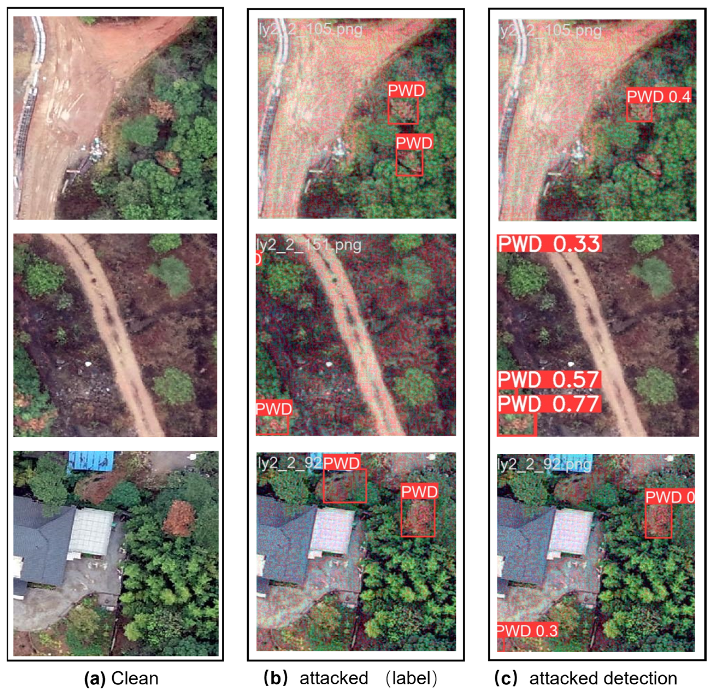
2.3.2. Adversarial Attack

Depending on the extent to which the attacker has knowledge of the model’s internal structure, adversarial attacks can be categorized into two types: white-box attacks [29,30] and black-box attacks [31,32]. In a white-box attack, the attacker has access to the training dataset, model architecture, parameters, and hyperparameters of the victim’s model. Lu et al. [33] proposed a white-box attack method against the Faster R-CNN object detector in 2017. The method is called DFool and is the first to demonstrate the existence of adversarial samples on object detectors. Furthermore, DFool may successfully transfer the adversarial samples from the digital dimension to the physical world and deceive the object detector. It is worth noting that the generated adversarial samples can be transferred to some extent to the YOLO 9000 detector. However, the method has certain requirements on the size of the perturbation and the contrast between the background and foreground. Chow et al. (2020) [34] introduced the TOG attack, which conducted adversarial attacks by reversing the training process. It performed well in various scenarios and was able to reduce the accuracy of the considered model on various datasets. Xie et al. (2017) [35] found that adding two or more heterogeneous perturbations significantly enhanced transferability, providing an effective method for black-box adversarial attacks on certain networks with unknown structures or attributes. The proposed DAG attack is designed for target detection and semantic segmentation tasks. Since DAG achieves adversarial samples by manipulating class labels to misclassify proposals specifically, its transferability is very poor and cannot work well on other regression-based detectors. In response to this issue, Wei et al. (2018) [36] pioneered the UEA method, which centered around integrating a generative adversarial network (GAN). They skillfully combined GANs, advanced classification losses, and lower-level feature losses to generate challenging adversarial examples. In the UEA method, the generator and discriminator of the GAN are introduced to generate adversarial examples and distinguish them. The generator is responsible for generating adversarial examples that can disrupt target detection systems, while the discriminator is responsible for judging the input image and distinguishing whether it is an adversarial example or a clean original image. Building upon the foundation of differentiable renderers, Wang et al. (2021) [37] introduced a novel adversarial attack called dual attention suppression (DAS). The goal of the DAS attack is to generate adversarial noise with stronger transferability and a more natural appearance. The core idea of DAS is to enhance transferability by utilizing the feature extraction network shared by one-stage and two-stage models. Additionally, to make the adversarial noise more natural, DAS attacks strive to keep the contour of the initial noise intact, while optimizing the adversarial noise to better align with the brain’s sensitivity to object contours.

2.3.3. Adversarial Defense

The core of adversarial sample attacks lies in finding small perturbations that can cause the model’s output category to change. Therefore, to defend against such attacks, the model needs to minimize its sensitivity to these small perturbations. Improving the training method of the model and optimizing the model’s internal structure are two approaches to defend against adversarial attacks. Adversarial training is a commonly used defense method, which enhances the robustness of the model by adding adversarial samples to the training set. This method can make the model more robust against minor perturbations and reduce the success rate of adversarial attacks. Shafahi et al. (2019) eliminated the additional overhead of generating adversarial samples by reusing the gradient information computed during the update of model parameters [38]. Zhang et al. (2019) [11] proposed a method of adversarial training for multi-task discriminative (MTD) sources aimed at enhancing the robustness of target detection models against adversarial attacks. This method is based on two separate sets of adversarial samples generated by single-task models, with the set that causes the largest overall task loss being selected for adversarial training. In this way, the model can better withstand various types of attacks and improve its reliability in real-world applications. Liu et al. (2020) proposed the Adversarial Noise Propagation (ANP) training algorithm, which enhanced the robustness of deep neural networks (DNNs) against adversarial samples and noise by injecting noise into the hidden layers [39]. Choi et al. (2022) [40] proposed a novel adversarial training strategy based on objectivity, which enhanced the robustness of detectors by utilizing objectivity loss. Considering objectivity in defense methods can significantly improve the robustness of detectors.

Another effective defense strategy is to improve the internal structure of the model. Enhancing the model’s defensive capabilities can be achieved by optimizing the architecture of the neural network. Gu et al. (2014) proposed adding noise and using denoising autoencoders (DAEs) for preprocessing to remove adversarial samples [41]. It includes a smoothness penalty in the end-to-end training process to enhance the network’s robustness against adversarial samples. Moosavi et al. (2018) proposed the CURE regularization method, which demonstrated a strong correlation between small curvature and robustness, thereby encouraging small curvature to enhance the robustness of the network [42]. Muthukumar et al. (2023) introduced the concept of sparse local Lipschitz property (SLL), which captured the stability of predictive variables under local perturbations and reduced the effective dimensionality [43]. When the Lipschitz constant was small, the model’s sensitivity to these small perturbations was also relatively low. By introducing regularization terms during training to encourage the model to have a smaller Lipschitz constant, the model could become more stable.

Despite the success achieved by the aforementioned defense methods, there are still some limitations. For instance, adversarial training typically requires substantial computing resources and time, and while it can enhance the model’s robustness against adversarial attacks, it may also have an adverse impact on its normal performance. Based on this, the authors propose a YOLOv5-DRCS model with an Adaptive Contraction Filter Network to further enhance the defense effect.

2.3.4. YOLOv5-DRCS

The researchers developed different versions of YOLOv5 based on model width and depth, including YOLOv5s, YOLOv5m, YOLOv5l, and YOLOv5x. The network architecture of YOLOv5 primarily consists of the following three parts: the backbone uses CSP-Darknet53, the neck part uses the more efficient spatial pyramid pooling Fast(SPPF) [44], and this fuses feature maps from different layers through up-sampling and down-sampling operations to generate multi-scale feature pyramids. To enhance the accuracy of object detection, it is common to use the neck part to combine feature maps of different levels to generate feature maps with multi-scale information. In the end, the generated feature map is sent to the head layer for detection, which consists of four modules: anchor, convolution, prediction, and non-maximum suppression. In this paper, the YOLOv5s master version is used as the basis for the detection model, with improvements being made on this basis. (Improved parts are in the red and blue boxes shown in Figure 5).

In YOLOv5, feature extraction is primarily performed by the backbone component. The backbone’s role is to transform the original input image into multi-layer feature maps, which are then used for subsequent object detection tasks. YOLOv5 uses the CSP-Model network as its feature extraction architecture. In this paper, the deep residual shrinking structure unit module is introduced into the CSP-Model’s Bottleneck module of the feature extraction module in YOLOv5. Figure 6 shows the details of the improved CSP feature extraction module. In the feature extraction stage, the interference on the image is treated as additive noise, and the clean feature image is obtained by processing the image using the improved CSP-Model.

The deep residual shrinking structure unit is used to deal with redundant information in data. In image recognition, redundant information manifests as image regions or features that are not directly related to the target. In the face of well-planned adversarial attacks, attackers often cleverly embed minor noises in the image that, while not visually significant, are sufficient to substantially interfere with the model’s decision-making process. By embedding the shrinking structure unit, these noise features can be identified and suppressed, thereby enhancing the model’s ability to resist interference. As illustrated in Figure 6a, the improved feature extraction module CSP-Model can be interpreted as a special self-attention mechanism, where the unimportant noise is set to zero through a soft thresholding process learned from the subnetwork. This method avoids manually setting thresholds, allowing each sample to have its own unique threshold.

The soft thresholding used in the deep residual shrinking structure unit is a commonly used thresholding method in signal and image processing. The soft thresholding operation compresses the lower part of the signal below the set threshold while keeping the higher part unchanged, thus retaining the key features such as edges and discontinuities in the signal. The small perturbations caused by adversarial attacks often blur or obscure the key features of the signal. By using soft thresholding, the noise part below the threshold is set to zero, reducing the impact of noise perturbations on the signal. Specifically, the computation formula for soft thresholding is as follows:

$$y=\left\{\begin{array}{l}x-\tau \hspace{0.25em}\hspace{0.25em}\hspace{0.25em}\hspace{0.25em}x>\tau \\ 0\hspace{1em}\hspace{1em}\hspace{0.25em}\hspace{0.25em}-\tau \le x\le \tau \\ x+\tau \hspace{0.25em}\hspace{0.25em}\hspace{0.25em}\hspace{0.25em}x<-\tau \end{array}\right.$$

(5)

where $x$ represents the input feature, $y$ represents the output feature, and $\tau$ is the threshold. The adjustable threshold property of the soft thresholding method enables it to customize strategies according to different application environments, whether to enhance feature fidelity or improve noise tolerance, ensuring that the model maintains efficient and stable performance in diverse adversarial environments. Soft thresholding converts numbers close to zero to zero, unlike ReLU which converts negative numbers to zero, allowing useful negative features to also be preserved [45]. According to Formula (6), it can be seen that the derivative of the soft threshold function is either zero or one:

$${\displaystyle \frac{\partial y}{\partial x}}=\left\{\begin{array}{l}1\hspace{0.25em}\hspace{0.25em}\hspace{0.25em}\hspace{0.25em}x>\tau \\ 0\hspace{0.25em}\hspace{0.25em}\hspace{0.25em}\hspace{0.25em}-\tau \le x\le \tau \\ 1\hspace{0.25em}\hspace{0.25em}\hspace{0.25em}\hspace{0.25em}x<-\tau \end{array}\right.$$

(6)

The threshold of the soft threshold is relatively difficult to be set manually and requires workers to have specialized knowledge in the field. With the continuous development of neural network technology, researchers proposed a deep residual shrinkage network that combines soft thresholding and residual networks, with a separate subnetwork used within the model to calculate the threshold values [46]. Residual neural networks (ResNet) solve the problem of gradient vanishing and network degradation by introducing residual connections, which allow the input to be directly passed to the output [47]. In ResNet, instead of directly mapping inputs to outputs, each convolutional layer adds inputs to outputs that span several layers, making the model easier to optimize through residual connections. The residual block is shown in Figure 7.

In the residual block, there are two 3 × 3 convolutional layers with the same number of output channels. Each convolution layer is followed by a batch normalization layer and ReLU activation function. Then, through the cross-layer data path, the two convolution operations are skipped and the input is added directly before the final ReLU activation function. Therefore, $\mathcal{F}\left(x\right)+x$ represents the output of input $x$ after convolution and activation functions; $\mathcal{F}\left(x\right)$ is then directly added to input $x$. The Residual Shrinkage Network is a combination network that includes a smaller subnetwork after the residual network, with the soft thresholding function serving as a nonlinear transformation layer inserted into the structural unit. The structural unit serves as a special module for calculating the threshold value. The following are the concrete steps for implementing the residual shrinkage structural unit in Figure 6b:

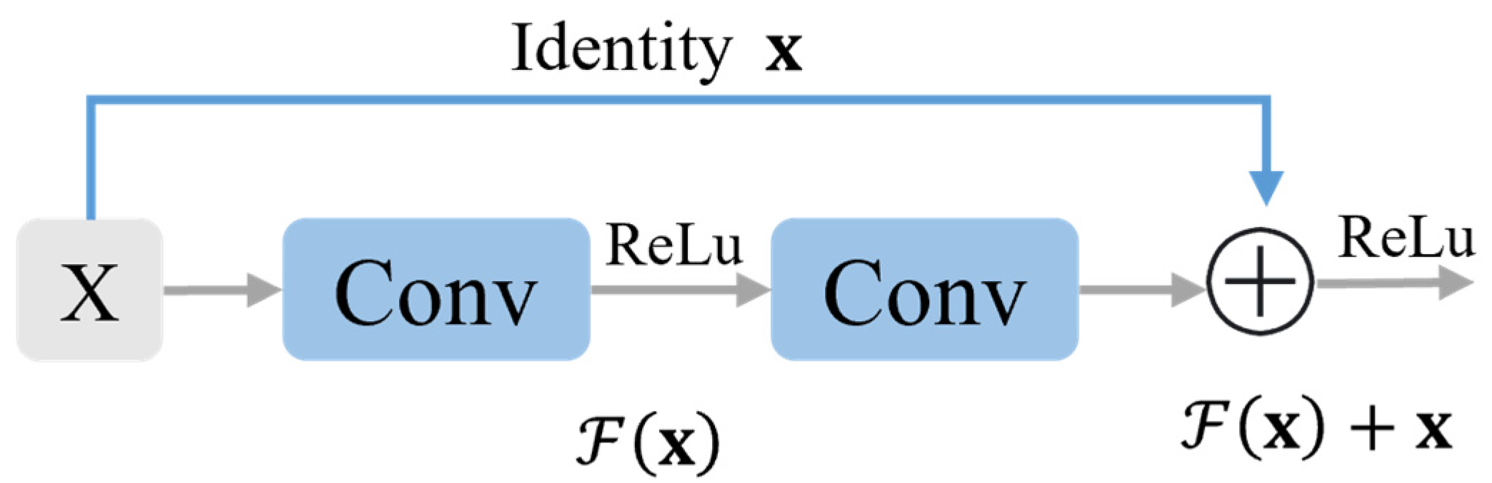
• After a series of convolutional operations, the feature $x^{\prime }$ is input into the subnetwork to obtain its absolute value $\left|x\right|$.
• The global average pooling (GAP) is performed on the absolute value $\left|x\right|$ of feature $x^{\prime }$ to obtain $\mid x{\mid }_{gap}$.
• Perform three steps for $\mid x{\mid }_{gap}$: Full connection (FC), batch normalization (BN), ReLu activation. Finally, the sigmoid function is used to normalize the output to between zero and one. The coefficient obtained is as follows:

  $$\alpha ={\displaystyle \frac{1}{1+e^{-z_C}}}$$

  (7)

  where $z_c$ is the characteristic of the c neuron.
• Finally, multiply the resulting coefficient α and $\mid x{\mid }_{gap}$ to obtain the final estimated threshold $k$:

  $$k=\alpha \cdot \underset{i,j}{average}\left|x_{i,j,c}\right|$$

  (8)

  where $k$ is the final threshold, and $i$, $j$, and $c$ are the width, height, and channel index of feature map $x$, respectively. By employing the aforementioned method, residual shrinkage modules are introduced into residual networks, ensuring that all thresholds are positive and preventing the output from being zero, thus keeping the thresholds within a reasonable range. Finally, the non-important features caused by noise removal are removed based on the threshold, and each output is compared with the corresponding threshold using the following formula to perform soft thresholding processing on the feature map:

  $$x=\left\{\begin{array}{l}{x}^{\prime }-k,\hspace{1em}\hspace{1em}{x}^{\prime }>k\\ 0,\hspace{1em}\hspace{1em}\hspace{1em}\hspace{1em}-k\le x^{\prime }\le k\\ x^{\prime }+k,\hspace{1em}\hspace{1em}{x}^{\prime }<k.\end{array}\right.$$

  (9)

During the fusion process between the backbone and neck, image feature extraction at the lower level may introduce a large amount of noise or irrelevant information. Due to the soft thresholding operation introduced in the backbone, the backbone network enhances its ability to extract edge features, but unavoidably causes minor perturbations to the feature image. To address this issue, the SimAM attention mechanism proposed by Yang et al. [48] is introduced in YOLOv5-DRSC. The SimAM attention mechanism does not introduce additional parameters, serving as a lightweight attention module that can be integrated into the overall architecture’s feature layer fusion process. The improved SimAM part of YOLOv5-DRCS is shown in the blue dashed box in Figure 5. When using attention mechanisms to dynamically adjust the focus on different regions of the image based on the task requirements, this refinement step is typically performed along the channel or spatial dimension. However, these methods generate only one or two dimensional weights, treating neurons equally in each channel or spatial location.

To enable the model to focus on more important regions in the image, reduce its attention to adversarial perturbations, and differentiate between subtle perturbations, the improved model in this paper includes a three-dimensional attention mechanism similar to SimAM. The underlying principle is to optimize an energy function such that each neuron is assigned a unique weight. The structure of the SimAM attention module is shown in Figure 8. Defining the energy function for each neuron can be achieved using the following equation:

$$e_t(w_t,b_t,\mathrm{y},x_i)=(y_t-\widehat{t}{)}^2+{\displaystyle \frac{1}{M-1}}\sum _{i=1}^{M-1}(y_o-{\widehat{x}}_i{)}^2$$

(10)

where $\widehat{t}$ and ${\widehat{x}}_i$ are linear transformations of $t$ and $x_i$, $t$ and $x_i$ refer to the target neuron and other neurons of input feature X, $i$ is an index of spatial dimension, and $W_t$ and $b_t$ refer to the weight and bias of a neuron transform, respectively. Introduce binary labels instead of $y_t$ and $y_o$, where $y_t=1,y_o=-1$. When $\widehat{t}$ is equal to $y_t$, Formula (9) reaches its minimum. By minimizing this equation, Formula (10) can find linear separability between the target neuron $t$ and all other neurons in the same channel [48]. The hyper-parameter $\lambda$ in Formula (11) is set to 0.0001. Finally, the energy function is defined as

$$e_t(w_t,b_t,\mathrm{y},x_i)={\displaystyle \frac{1}{M-1}}\sum _{i=1}^{M-1}(-1-(w_t{x}_i+b_t){)}^2+(1-(w_{t}t+b_t){)}^2+\lambda w_t^2$$

(11)

The above formula has the following solution:

$$w_t=-{\displaystyle \frac{2\left(t-{\mu }_t\right)}{{\left(t-{\mu }_t\right)}^2+2{\sigma }_t^2+2\lambda }},$$

(12)

$$b_t=-{\displaystyle \frac{1}{2}}(t+{\mu }_t)w_t.$$

(13)

where ${\mu }_t={\displaystyle \frac{1}{M-1}}\sum _{i=1}^{M-1}{x}_i$ and ${\sigma }_t^2={\displaystyle \frac{1}{M-1}}\sum _i^{M-1}(x_i-{\mu }_t{)}^2$ are the mean and variance of all neurons in the channel except $t$. Since the existing solutions in Formulas (11) and (12) are obtained on individual channels, it is reasonable to assume that all pixels in a single channel follow the same distribution. Therefore, the minimum energy can be obtained using the following formula:

$$e_t^{*}={\displaystyle \frac{4({\widehat{\sigma }}^2+\lambda )}{{\left(t-\widehat{\mu }\right)}^2+2{\widehat{\sigma }}^2+2\lambda }}.$$

(14)

where $\widehat{\mu }={\displaystyle \frac{1}{M}}\sum _{i=1}^M{x}_i$ and ${\widehat{\sigma }}^2={\displaystyle \frac{1}{M}}\sum _{i=1}^M(x_i-\widehat{\mu }{)}^2.$ Formula (13) means that the lower the energy, the greater the difference between neuron t and the surrounding neurons and the higher the importance. Therefore, the importance of neurons can be obtained through ${\displaystyle \frac{1}{e_t^{\mathrm{*}}}}$.

3. Results and Discussion

3.1. Experimental Setup and Model Training

The experimental parameters and experimental environment used in the study are shown in

Table 2. The training parameters.

Training Parameters	Details
Epochs	150
Image size (pixel)	320 × 320
batch size	32
Initial learning rate	0.01
Final OneCycleLR learning rate	0.1
Optimization algorithm and parameters	Adam (0.937)
Weight decay	0.0005
Epochs	150

and

Table 3. The experimental environment.

Experimental Environment	Details
Programming language	Python 3.8
Operating system	Windows 11
Deep learning framework	Pytorch 1.11.0
CPU	22 vCPU AMD EPYC 7T83 64-Core
GPU	NVIDIA GeForce RTX 4090

. Before training the dataset, the parameters of the YOLOv5 network are initialized. Both YOLOv5 and YOLOV5-DRCS models perform transfer training based on pre-training models. During the training process, each model is saved at its optimal convergence point and tested on a test set to evaluate its performance. In this paper, mAP and Recall indexes are used to evaluate the robustness of the model on adversarial sample datasets. For this study, an IoU detection threshold of 0.5 is used, hence the evaluation criterion is [email protected]. Figure 9a shows the convergence results during model training, and Figure 9b shows the mAP and precision values during model training.

Table 4. Performance metrics for each model on the PWT clean dataset.

Model	[email protected]	Recall	GFLOPs	FPS	Params (M)
YOLOv5s	94.0	89.1	16.0	71.5	7.02
YOLOv5m	89.2	81.8	47.9	40.5	20.8
YOLOv5l	92.2	86.3	107.7	24.1	46.1
YOLOv5-DRCS	93.5	86.9	15.8	69.0	7.07

shows the performance metrics for each model on the PWT clean dataset.

$$Precision={\displaystyle \frac{TP}{TP+FP}}\times 100\mathrm{\%}$$

(15)

$TP$ means that the amount is predicted correctly. As the accuracy increases, the number of FPS decreases, with $FP$ meaning that a healthy pine tree is less likely to be mistaken for a diseased one.

$$Recall={\displaystyle \frac{TP}{TP+FN}}\times 100\mathrm{\%}$$

(16)

$Recall$ rate indicates the probability that diseased pine trees are actually predicted. TP means that the amount is predicted correctly. As the accuracy improves, $FN$ means that the diseased tree is incorrectly predicted to be a healthy tree.

$$mAP={\displaystyle \frac{\sum _n^{i=1}{A}_{i}P}{n}}$$

(17)

$mAP$ represents the $Precision$ accuracy of the detection process. [email protected] represents the average precision at an intersection over an IoU criterion of 0.5.

3.2. Attack Experiment and Analysis

In this section, the authors examine the vulnerability of the model to attack localization tasks. By measuring the model’s accuracy under different proportions of adversarial samples, the authors evaluate its ability to resist adversarial attacks and its overall performance in object detection. The authors work under the assumption that as the model deepens, it becomes more vulnerable to adversarial attacks against gradients. The proposed YOLOV5-DRCS model was compared with YOLOv5 models of different widths and depths. The attack algorithm step size is $\alpha$ = 1 and the number of iterations is $T$ = 1. Detailed results of the comparative experiments are shown in

Table 5. Model mAP when 40% of samples are attacked.

Method	Att. Size	YOLOv5s	YOLOv5m	YOLOv5l	YOLOv5-DRCS
FGSM	$ϵ$ = 2	92.7	91.7	91.8	92.4
	$ϵ$ = 4	88.7	88.2	90.2	92.5
	$ϵ$ = 6	85.3	85.4	91.4	91.0
	$ϵ$ = 8	75.9	75.2	85.5	90.1

,

Table 6. Model mAP when 70% of samples are attacked.

Method	Att. Size	YOLOv5s	YOLOv5m	YOLOv5l	YOLOv5-DRCS
FGSM	$ϵ$ = 2	85.8	90.3	91.9	89.6
	$ϵ$ = 4	81.4	86.9	87.2	89.0
	$ϵ$ = 6	78.1	78.9	81.7	87.1
	$ϵ$ = 8	74.1	66.3	74.0	82.1

and

Table 7. Model mAP when 100% of samples are attacked.

Method	Att. Size	YOLOv5s	YOLOv5m	YOLOv5l	YOLOv5-DRCS
FGSM	$ϵ$ = 2	81.1	86.9	86.5	88.1
	$ϵ$ = 4	77.1	80.2	86.8	86.5
	$ϵ$ = 6	67.7	64.9	74.5	84.0
	$ϵ$ = 8	54.0	54.5	65.8	77.2

indicating mAP changes in the dataset are caused by different adversarial sample proportions (40%, 70%, 100%) with the attack coefficient $ϵ$ being 2, 4, 6, 8.

The experimental results show that when only 40% of the dataset is augmented with adversarial samples, the detection model maintains a relatively stable accuracy. However, as the proportion of adversarial samples increases, especially when it reaches 100%, the performance of all models declines significantly. The proposed YOLOv5-DRCS model can maintain a mAP of 88.1%, 86.5%, 84.0%, and 77.2% at attack coefficients $ϵ$ of 2, 4, 6, and 8, respectively.

To more comprehensively validate the robustness of the YOLOv5-DRCS model, beyond testing with the FGSM attack, the authors extended the experimental scope by incorporating three gradient-based adversarial attack methods: I-FGSM [10], MI-FGSM [49], and PGD. The I-FGSM, an iterative version of the FGSM, generates adversarial samples by iteratively applying smaller perturbations. Compared to the FGSM, the I-FGSM can produce adversarial samples that are harder for models to defend against, as it allows for the accumulation of smaller gradient changes in each iteration, gradually approaching the optimal adversarial perturbation. The MI-FGSM introduces a momentum mechanism on top of the I-FGSM to stabilize the update direction and accelerate the convergence process. It updates the gradient in the current iteration by accumulating gradient information from previous iterations, thereby avoiding local optima and generating more destructive adversarial samples.

In experiments, three types of attacks were applied to the YOLOv5 DRCS model and comparative model. The attacked sample ratio in the test set was 100%, and the performance of the model is recorded under each attack. As shown in

Table 8. Model’s [email protected], using I-FGSM, MI-FGSM, and PGD attacks.

Method	Att. Size	YOLOv5s	YOLOv5m	YOLOv5l	YOLOv5-DRCS
I-FGSM	$ϵ$ = 2	89.2	85.5	84.1	86.7
	$ϵ$ = 4	78.5	70.6	71.7	79.0
	$ϵ$ = 6	61.9	60.4	58.3	65.8
	$ϵ$ = 8	45.9	50.6	47.4	47.2
MI-FGSM	$ϵ$ = 2	82.9	82.6	82.0	84.2
	$ϵ$ = 4	74.3	71.6	70.7	75.8
	$ϵ$ = 6	64.8	64.0	61.4	68.3
	$ϵ$ = 8	50.3	48.9	46.3	52.2
PGD	$ϵ$ = 2	78.4	72.8	73.0	78.8
	$ϵ$ = 4	61.5	58.1	57.4	60.0
	$ϵ$ = 6	43.4	51.8	47.0	51.2
	$ϵ$ = 8	31.0	43.9	40.5	38.3

, in most cases, the YOLOv5-DRCS model still demonstrated good defensive capabilities.

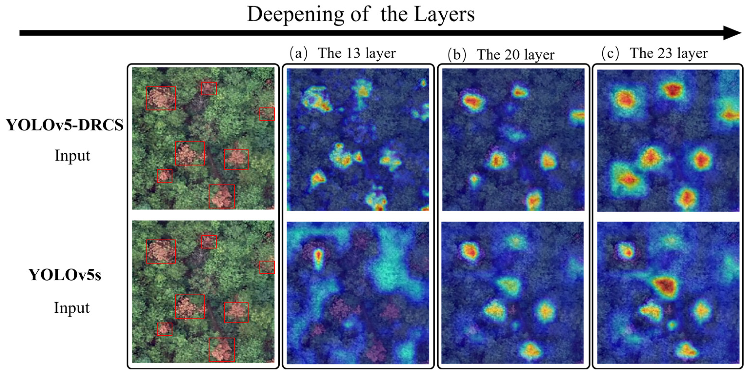
3.3. Gradient-Weighted Class Activation Mapping Analysis

Gradient-weighted class Activation Mapping (Grad-CAM) provides an effective visual interpretation method for convolutional neural network decisions, which can help to understand the process of model decision-making [50]. By showing the areas of the image that the model focuses on, Grad-CAM can help identify the basis of the model for classification and prediction. This helps to enhance the interpretability and reliability of the model and helps developers better understand the model’s performance and potential limitations [51]. It generates a coarse heatmap by taking the average of the gradients of the output classes with respect to the outputs of a specific convolutional layer and multiplying them by the outputs of that layer. The heatmap is used to display the areas of the image that the model is focusing on. The formula for this can be simply expressed as follows:

$${\mathrm{L}}_{\mathrm{G}\mathrm{r}\mathrm{a}\mathrm{d}-\mathrm{C}\mathrm{A}\mathrm{M}}^{\mathrm{c}}=\mathrm{R}\mathrm{e}\mathrm{L}\mathrm{U}(\sum _{\mathrm{i}}\sum _{\mathrm{j}}{\displaystyle \frac{\partial {\mathrm{Y}}^{\mathrm{c}}}{\partial {\mathrm{A}}_{\mathrm{i}\mathrm{j}}}}{\mathrm{A}}_{\mathrm{i}\mathrm{j}})$$

(18)

where ${\mathrm{Y}}^{\mathrm{c}}$ represents the score for a particular category of model output, ${\displaystyle \frac{\partial {\mathrm{Y}}^{\mathrm{c}}}{\partial {\mathrm{A}}_{\mathrm{i}\mathrm{j}}}}$ is the gradient of the score for this category against feature map $\mathrm{A}$, and ${\mathrm{A}}_{\mathrm{i}\mathrm{j}}$ denotes the element in feature map $\mathrm{A}$ at row $\mathrm{i}$ and column $\mathrm{j}$. By performing a summation operation, we obtain the weight for each channel, followed by the ReLU function for nonlinear mapping.

Therefore, to further enhance the explainability of the YOLOv5-DRCS model, we included the effects of the improved CSP-module and the fusion of the SimAM attention layer. By conducting experiments, the results of the improved YOLOv5-DRCS and YOLOv5s’ NECK section layers 13, 20, and 23 were compared with each other. As shown in Figure 10, in Grad-CAM, the deeper red shadows indicate that the model pays high attention to these regions of the image. The yellow areas represent lower but still significant attention levels, while the blue areas contain redundant and interfering information. As shown in Figure 10b, with the improved CSP-module and attention mechanism integrated, the blue area decreases, and the model becomes more sensitive to features related to the infected tree, accurately identifying the region of interest. In contrast, the YOLOv5 model had a larger attention area focused on infected trees, was more susceptible to adversarial perturbations, and even resulted in obvious false alarms. As shown in Figure 10c, the improved model YOLOv5-DRCS’s Grad-CAM not only provides more precise attention regions but also exhibits higher attention. This indicates that the model proposed in this paper can effectively distinguish targets and defend against adversarial perturbations.

3.4. Adversarial Training Results

In the attack experiment in the previous section, the instability of the model against the attack as the disturbance coefficient increases is discussed. As the proportion of adversarial samples added increases to 70% and 100%, the precision of all experimental models will begin to decline significantly once the perturbation coefficient $ϵ$ exceeds 4. This result highlights the importance of selecting an appropriate perturbation coefficient for adversarial training defense. In this section’s experiments, the authors attempt to select different levels of attack coefficient $ϵ$ are 2, 4, 6, and 8 to perturb the coefficients in the training set and add different proportions of adversarial samples for adversarial training, aiming to study the effectiveness of using different attack coefficients for adversarial training.

Figure 11a–d shows the accuracy curves obtained by training the model using adversarial samples with interference strengths of 2, 4, 6, and 8, respectively, and testing them on the corresponding test sets. To diversify the attack scenarios, the attack sample proportion in the test set was set to 40%, 70%, and 100%. Figure 11a corresponds to $ϵ$ = 2, Figure 11b corresponds to $ϵ$ = 4, Figure 11c corresponds to $ϵ$ = 6, and Figure 11d corresponds to $ϵ$ = 8.

The analysis across all the charts indicates that the proportion of adversarial samples significantly affects the detection performance of the model. The stability of the model gradually decreases with the increase in the proportion of adversarial attack samples. However, as the disturbance coefficient used by the training sample increases, the accuracy of the model is unstable, as shown in Figure 11d. By incorporating adversarial samples into the model training phase, a certain degree of regularization can be achieved for neural networks. However, training the network to fit both normal samples and perturbed samples can lead the model to learn features that are sensitive to the perturbations. In practical applications, the appropriate level of the perturbation coefficient should be selected for adversarial training based on the specific dataset and attack type.

3.5. Model Detection Results Image

Figure 12 shows the comparison of the detection results of YOLOv5-DRCS and YOLOv5s models of different depths in real scenarios. Add the disturbance coefficient $ϵ=6$. Compared to the detection results of the contrastive models shown in Figure 12c,e, the detection results of the proposed YOLOv5-DRCS model show a significant reduction in false alarms or missed detections, further verifying the previously proposed view that as the model depth increases, the model becomes more susceptible to adversarial attacks targeting the gradients.

4. Conclusions

With the large-scale application of UAV technology, the potential attack risk of forestry remote sensing image is increasing. Aiming at the challenge of forestry UAV remote sensing target recognition in insecure environments, the author proposes an improved YOLOV5-DRCS model based on YOLOv5. The visualization analysis of the improved part is carried out using the Grad-CAM method. The attack dataset generated by the FGSM is used for adversarial training, and the appropriate disturbance coefficient is selected to maintain the effectiveness of adversarial training. The residual contraction subnetwork is introduced to achieve the self-adaptive filtering of anti-disturbance in feature extraction. In the feature fusion stage, the SimAM attention mechanism is used to calculate the three-dimensional attention weight for the possible subtle disturbance, so as to reduce the model’s attention to the subtle disturbance. The robustness of YOLOv5-DRCS against FGSM attacks is verified by experiments. To evaluate the performance against adversarial attacks, YOLOv5 models of different depths and the improved model YOLOV5-DRCS have been tested.

References

1. Ikegami, M.; Jenkins, T.A. Estimate global risks of a forest disease under current and future climates using species distribution model and simple thermal model—Pine Wilt disease as a model case. For. Ecol. Manag. 2018, 409, 343–352. [Google Scholar] [CrossRef]
2. Kuang, J.; Yu, L.; Zhou, Q.; Wu, D.; Ren, L.; Luo, Y. Identification of Pine Wilt Disease-Infested Stands Based on Single- and Multi-Temporal Medium-Resolution Satellite Data. Forests 2024, 15, 596. [Google Scholar] [CrossRef]
3. Zhang, X.; Yang, H.; Cai, P.; Chen, G.; Li, X.; Zhu, K. A review on the research progress and methodology of remote sensing for monitoring pine wood nematode disease. J. Agric. Eng. 2022, 18, 184–194. [Google Scholar]
4. Li, H.; Wang, Y. Influence of environmental factors on UAV image recognition accuracy for pine wilt disease. For. Res. 2019, 32, 102–110. [Google Scholar]
5. Szegedy, C.; Zaremba, W.; Sutskever, I.; Bruna, J.; Erhan, D.; Goodfellow, I.; Fergus, R. Intriguing properties of neural networks. arXiv 2013, arXiv:1312.6199. [Google Scholar]
6. Goodfellow, I.J.; Shlens, J.; Szegedy, C. Explaining and harnessing adversarial examples. arXiv 2014, arXiv:1412.6572. [Google Scholar]
7. Boloor, A.; He, X.; Gill, C.; Vorobeychik, Y.; Zhang, X. Simple Physical Adversarial Examples against End-to-End Autonomous Driving Models. In Proceedings of the 2019 IEEE International Conference on Embedded Software and Systems (ICESS), Las Vegas, NV, USA, 2–3 June 2019; pp. 1–7. [Google Scholar] [CrossRef]
8. Moosavi-Dezfooli, S.-M.; Fawzi, A.; Frossard, P. DeepFool: A Simple and Accurate Method to Fool Deep Neural Networks. In Proceedings of the 2016 IEEE Conference on Computer Vision and Pattern Recognition (CVPR), Las Vegas, NV, USA, 27–30 June 2016; pp. 2574–2582. [Google Scholar] [CrossRef]
9. Madry, A.; Makelov, A.; Schmidt, L.; Tsipras, D.; Vladu, A. Towards deep learning models resistant to adversarial attacks. In Proceedings of the 6th International Conference on Learning Representations, ICLR 2018—Conference Track Proceedings, Vancouver, BC, Canada, 30 April–3 May 2018. [Google Scholar]
10. Kurakin, A.; Goodfellow, I.J.; Bengio, S. Adversarial examples in the physical world. arXiv 2016, arXiv:1607.02533. [Google Scholar]
11. Zhang, H.; Wang, J. Towards Adversarially Robust Object Detection. In Proceedings of the 2019 IEEE/CVF International Conference on Computer Vision (ICCV), Seoul, Republic of Korea, 27 October–2 November 2019; pp. 421–430. [Google Scholar] [CrossRef]
12. Wang, J.; Chen, R.F.; Chen, Q.; Li, Y.H.; Zhang, C. Research on Forest Parameter Information Extraction Progress Driven by UAV Remote Sensing Technology. For. Resour. Manag. 2020, 5, 144–151. [Google Scholar]
13. Huang, T.; Zhang, Q.; Liu, J.; Hou, R.; Wang, X.; Li, Y. Adversarial attacks on deep-learning-based SAR image target recognition. J. Netw. Comput. Appl. 2020, 162, 102632. [Google Scholar] [CrossRef]
14. Yuan, X.; He, P.; Zhu, Q.; Li, X. Adversarial Examples: Attacks and Defenses for Deep Learning. IEEE Trans. Neural Netw. Learn. Syst. 2019, 30, 2805–2824. [Google Scholar] [CrossRef]
15. Best, K.L.; Schmid, J.; Tierney, S.; Awan, J.; Beyene, N.; Holliday, M.A.; Khan, R.; Lee, K. How to Analyze the Cyber Threat from Drones: Background, Analysis Frameworks, and Analysis Tools; Rand Corp.: Santa Monica, CA, USA, 2020. [Google Scholar]
16. Kwon, Y.-M. Vulnerability Analysis of the Mavlink Protocol for Unmanned Aerial Vehicles. Master’s Thesis, DGIST, Daegu, Republic of Korea, 2018. [Google Scholar] [CrossRef]
17. Highnam, K.; Angstadt, K.; Leach, K.; Weimer, W.; Paulos, A.; Hurley, P. An Uncrewed Aerial Vehicle Attack Scenario and Trustworthy Repair Architecture. In Proceedings of the 2016 46th Annual IEEE/IFIP International Conference on Dependable Systems and Networks Workshop (DSN-W), Toulouse, France, 28 June–1 July 2016; pp. 222–225. [Google Scholar] [CrossRef]
18. Syifa, M.; Park, S.J.; Lee, C.W. Detection of the Pine Wilt Disease Tree Candidates for Drone Remote Sensing Using Artificial Intelligence Techniques. Engineering 2020, 6, 919–926. [Google Scholar] [CrossRef]
19. Iordache, M.-D.; Mantas, V.; Baltazar, E.; Pauly, K.; Lewyckyj, N. A Machine Learning Approach to Detecting Pine Wilt Disease Using Airborne Spectral Imagery. Remote Sens. 2020, 12, 2280. [Google Scholar] [CrossRef]
20. Oide, A.H.; Nagasaka, Y.; Tanaka, K. Performance of machine learning algorithms for detecting pine wilt disease infection using visible color imagery by UAV remote sensing. Remote Sens. Appl. Soc. Environ. 2022, 28, 100869. [Google Scholar] [CrossRef]
21. Yu, R.; Luo, Y.; Zhou, Q.; Zhang, X.; Wu, D.; Ren, L. Early detection of pine wilt disease using deep learning algorithms and UAV-based multispectral imagery. For. Ecol. Manag. 2021, 497, 119493. [Google Scholar] [CrossRef]
22. Zhang, R.; You, J.; Lee, J. Detecting Pine Trees Damaged by Wilt Disease Using Deep Learning Techniques Applied to Multi-Spectral Images. IEEE Access 2022, 10, 39108–39118. [Google Scholar] [CrossRef]
23. Yao, J.; Song, B.; Chen, X.; Zhang, M.; Dong, X.; Liu, H.; Liu, F.; Zhang, L.; Lu, Y.; Xu, C.; et al. Pine-YOLO: A Method for Detecting Pine Wilt Disease in Unmanned Aerial Vehicle Remote Sensing Images. Forests 2024, 15, 737. [Google Scholar] [CrossRef]
24. Wu, W.; Zhang, Z.; Zheng, L.; Han, C.; Wang, X.; Xu, J.; Wang, X. Research Progress on the Early Monitoring of Pine Wilt Disease Using Hyperspectral Techniques. Sensors 2020, 20, 3729. [Google Scholar] [CrossRef]
25. Li, M.; Li, H.; Ding, X.; Wang, L.; Wang, X.; Chen, F. The Detection of Pine Wilt Disease: A Literature Review. Int. J. Mol. Sci. 2022, 23, 10797. [Google Scholar] [CrossRef]
26. Carlini, N.; Wagner, D. Towards Evaluating the Robustness of Neural Networks. In Proceedings of the 2017 IEEE Symposium on Security and Privacy (SP), San Jose, CA, USA, 22–24 May 2017; pp. 39–57. [Google Scholar] [CrossRef]
27. Liao, F.; Liang, M.; Dong, Y.; Pang, T.; Hu, X.; Zhu, J. Defense against Adversarial Attacks Using High-Level Representation Guided Denoiser. In Proceedings of the 2018 IEEE/CVF Conference on Computer Vision and Pattern Recognition, Salt Lake City, UT, USA, 18–23 June 2018. [Google Scholar] [CrossRef]
28. Chiang, P.Y.; Curry, M.; Abdelkader, A.; Kumar, A.; Dickerson, J.; Goldstein, T. Detection as regression: Certified object detection with median smoothing. Adv. Neural Inf. Process. Syst. 2020, 33, 1275–1286. [Google Scholar]
29. Won, J.; Seo, S.-H.; Bertino, E. A Secure Shuffling Mechanism for White-Box Attack-Resistant Unmanned Vehicles. IEEE Trans. Mob. Comput. 2019, 19, 1023–1039. [Google Scholar] [CrossRef]
30. Xu, L.; Zhai, J. DCVAE-adv: A Universal Adversarial Example Generation Method for White and Black Box Attacks. Tsinghua Sci. Technol. 2024, 29, 430–446. [Google Scholar] [CrossRef]
31. YShi, Y.; Han, Y.; Hu, Q.; Yang, Y.; Tian, Q. Query-Efficient Black-Box Adversarial Attack With Customized Iteration and Sampling. IEEE Trans. Pattern Anal. Mach. Intell. 2022, 45, 2226–2245. [Google Scholar] [CrossRef]
32. Li, C.; Wang, H.; Zhang, J.; Yao, W.; Jiang, T. An Approximated Gradient Sign Method Using Differential Evolution for Black-Box Adversarial Attack. IEEE Trans. Evol. Comput. 2022, 26, 976–990. [Google Scholar] [CrossRef]
33. Lu, J.; Sibai, H.; Fabry, E. Adversarial examples that fool detectors. arXiv 2017, arXiv:1712.02494. [Google Scholar]
34. Chow, K.-H.; Liu, L.; Loper, M.; Bae, J.; Gursoy, M.E.; Truex, S.; Wei, W.; Wu, Y. TOG: Targeted Adversarial Objectness Gradient Attacks on Real-time Object Detection Systems. arXiv 2020, arXiv:2004.04320. [Google Scholar]
35. Xie, C.; Wang, J.; Zhang, Z.; Zhou, Y.; Xie, L.; Yuille, A. Adversarial Examples for Semantic Segmentation and Object Detection. In Proceedings of the 2017 IEEE International Conference on Computer Vision (ICCV), Venice, Italy, 22–29 October 2017; pp. 1378–1387. [Google Scholar] [CrossRef]
36. Wei, X.; Liang, S.; Chen, N.; Cao, X. Transferable Adversarial Attacks for Image and Video Object Detection. In Proceedings of the International Joint Conference on Artificial Intelligence, Stockholm, Sweden, 13–19 July 2018. [Google Scholar] [CrossRef]
37. Wang, J.; Liu, A.; Yin, Z.; Liu, S.; Tang, S.; Liu, X. Dual attention suppression attack: Generate adversarial camouflage in physical world. In Proceedings of the IEEE/CVF Conference on Computer Vision and Pattern Recognition, New Orleans, LA, USA, 18–24 June 2021; pp. 8565–8574. [Google Scholar]
38. Shafahi, A.; Najibi, M.; Ghiasi, M.A.; Xu, Z.; Dickerson, J.; Studer, C.; Davis, L.S.; Taylor, G.; Goldstein, T. Adversarial training for free! In Proceedings of the Advances in Neural Information Processing Systems 32, Vancouver, BC, Canada, 8–14 December 2019; pp. 3353–3364. [Google Scholar]
39. Liu, A.; Liu, X.; Yu, H.; Zhang, C.; Liu, Q.; Tao, D. Training Robust Deep Neural Networks via Adversarial Noise Propagation. IEEE Trans. Image Process. 2021, 30, 5769–5781. [Google Scholar] [CrossRef] [PubMed]
40. Choi, J.I.; Tian, Q. Adversarial Attack and Defense of YOLO Detectors in Autonomous Driving Scenarios. In Proceedings of the 2022 IEEE Intelligent Vehicles Symposium (IV), Aachen, Germany, 5–9 June 2022; pp. 1011–1017. [Google Scholar] [CrossRef]
41. Gu, S.; Rigazio, L. Towards deep neural network architectures robust to adversarial examples. arXiv 2014, arXiv:1412.5068. [Google Scholar]
42. Moosavi-Dezfooli, S.-M.; Fawzi, A.; Uesato, J.; Frossard, P. Robustness via Curvature Regularization, and Vice Versa. In Proceedings of the 2019 IEEE/CVF Conference on Computer Vision and Pattern Recognition (CVPR), Long Beach, CA, USA, 16–20 June 2019; pp. 9070–9078. [Google Scholar] [CrossRef]
43. Muthukumar, R.; Sulam, J. Adversarial robustness of sparse local lipschitz predictors. arXiv 2022, arXiv:2202.13216. [Google Scholar] [CrossRef]
44. Tang, H.; Liang, S.; Yao, D.; Qiao, Y. A visual defect detection for optics lens based on the YOLOv5-C3CA-SPPF network model. Opt. Express 2023, 31, 2628–2643. [Google Scholar] [CrossRef]
45. Donoho, D.L. De-noising by soft-thresholding. IEEE Trans. Inf. Theory 1995, 41, 613–627. [Google Scholar] [CrossRef]
46. Zhao, M.; Zhong, S.; Fu, X.; Tang, B.; Pecht, M. Deep Residual Shrinkage Networks for Fault Diagnosis. IEEE Trans. Ind. Informatics 2019, 16, 4681–4690. [Google Scholar] [CrossRef]
47. He, K.; Zhang, X.; Ren, S.; Sun, J. Deep Residual Learning for Image Recognition. In Proceedings of the 2016 IEEE Conference on Computer Vision and Pattern Recognition (CVPR), Las Vegas, NV, USA, 27–30 June 2016; pp. 770–778. [Google Scholar] [CrossRef]
48. Yang, L.; Zhang, R.Y.; Li, L.; Xie, X. Simam: A simple, parameter-free attention module for convolutional neural networks. In Proceedings of the International Conference on Machine Learning, Virtual, 18–24 July 2021. [Google Scholar]
49. Dong, Y.; Liao, F.; Pang, T.; Su, H.; Zhu, J.; Hu, X.; Li, J. Boosting Adversarial Attacks with Momentum. In Proceedings of the 2018 IEEE/CVF Conference on Computer Vision and Pattern Recognition, Salt Lake City, UT, USA, 18–23 June 2018; pp. 9185–9193. [Google Scholar]
50. Selvaraju, R.R.; Cogswell, M.; Das, A.; Vedantam, R.; Parikh, D.; Batra, D. Grad-CAM: Visual Explanations from Deep Networks via Gradient-Based Localization. In Proceedings of the 2017 IEEE International Conference on Computer Vision (ICCV), Venice, Italy, 22–29 October 2017; pp. 618–626. [Google Scholar] [CrossRef]
51. Chu, J.; Cai, J.; Li, L.; Fan, Y.; Su, B. Bilinear Feature Fusion Convolutional Neural Network for Distributed Tactile Pressure Recognition and Understanding via Visualization. IEEE Trans. Ind. Electron. 2021, 69, 6391–6400. [Google Scholar] [CrossRef]
Figure 1. The UAV was attacked when it was operating.
Forests 15 01623 g001
Figure 2. Study area and sampling area.
Forests 15 01623 g002
Figure 3. The construction process of the dataset.
Forests 15 01623 g003
Figure 4. (a) represents an undisturbed original image. (b) represents the attacked image and the true label, with a visually imperceptible minor perturbation on the attacked image. (c) indicates that when the attacked image in (b) is input into the undefended detection model, the detection target cannot be found and the detection target is located incorrectly.
Forests 15 01623 g004
Figure 5. The YOLOv5-DRCS model structure.
Forests 15 01623 g005
Figure 6. (a) illustrates the overall structure of the improved CSP-Model module, while (b) depicts the improved Bottleneck structure, where the feature layer input is fed into a subnetwork to adaptively compute a set of thresholds, which are then applied to the attention weights of the feature layer to filter out noisy interference. ⊗ denotes the final estimated threshold k obtained after α calculation, and ⊕ denotes cross-layer connection.
Forests 15 01623 g006
Figure 7. Residual block.
Forests 15 01623 g007
Figure 8. SimAM attention mechanism.
Forests 15 01623 g008
Figure 9. (a) Network training and validation loss convergence results. (b) [email protected] and precision for network training.
Forests 15 01623 g009
Figure 10. Comparison of Gradient-Weighted Class Activation Mapping.
Forests 15 01623 g010
Figure 11. Adversarial training when the disturbance coefficients are 2, 4, 6, and 8. (a) corresponds to ϵ = 2, (b) corresponds to ϵ = 4, (c) corresponds to ϵ = 6, and (d) corresponds to ϵ = 8.
Forests 15 01623 g011
Figure 12. Detection results of YOLOv5-DRCS, YOLOv5s, YOLOv5m, and YOLOv5l.
Forests 15 01623 g012