

Three-Dimensional Reconstruction of Forest Scenes with Tree–Shrub–Grass Structure Using Airborne LiDAR Point Cloud


Abstract
:1. Introduction
2. Materials
2.1. Study Area
2.2. ALS Point Cloud
2.3. Validation Data
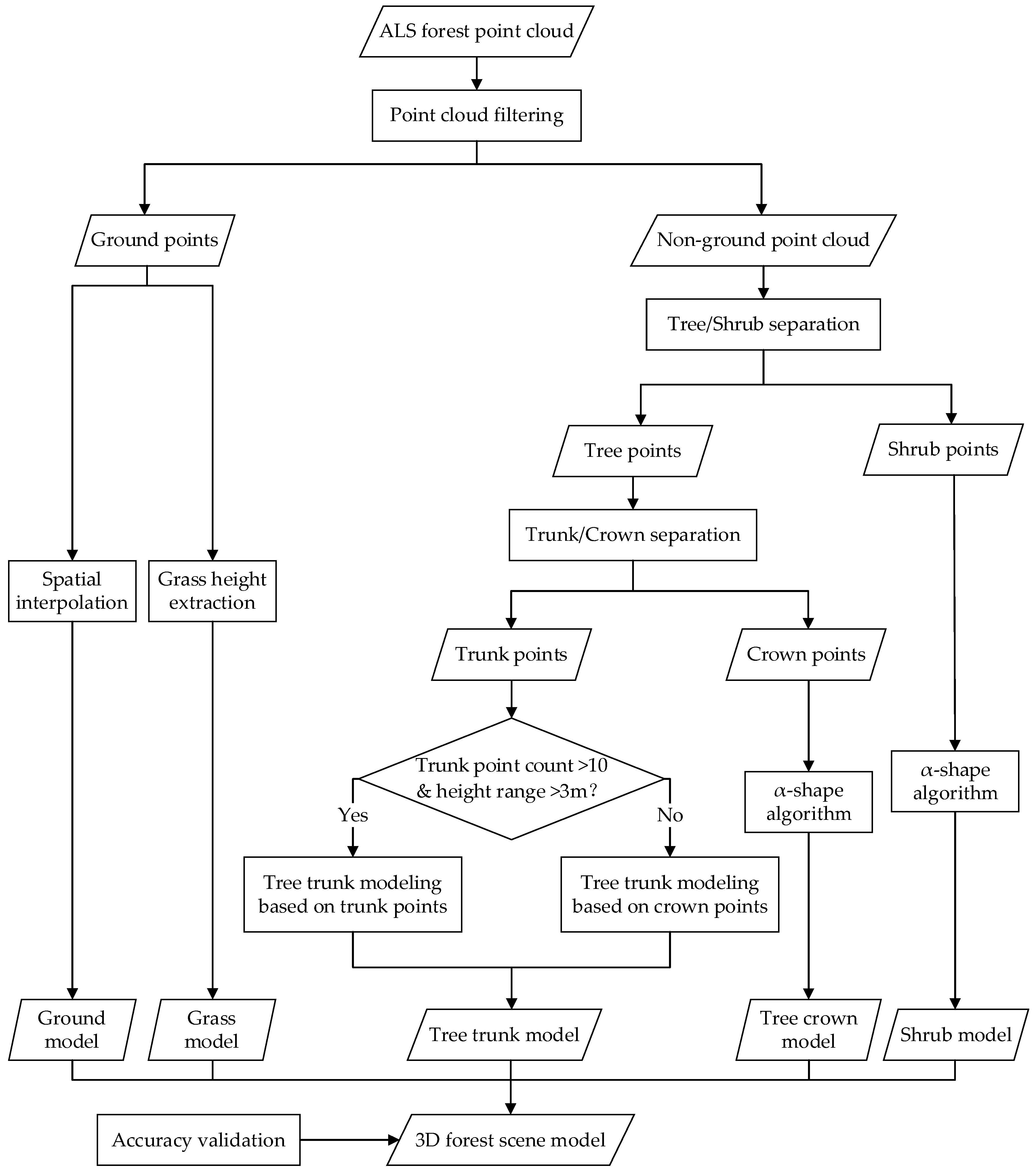
3. Methods
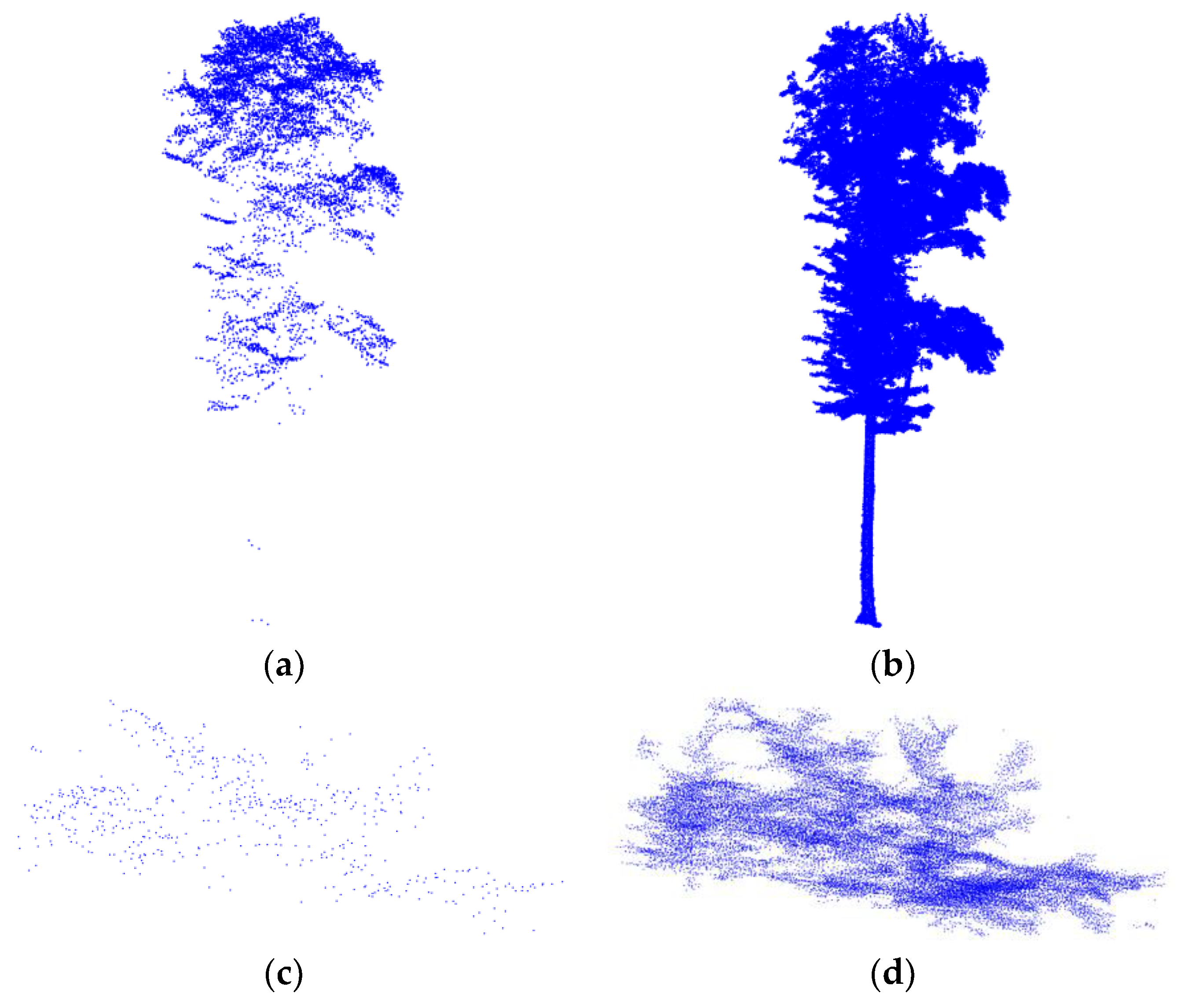
3.1. Point Cloud Segmentation
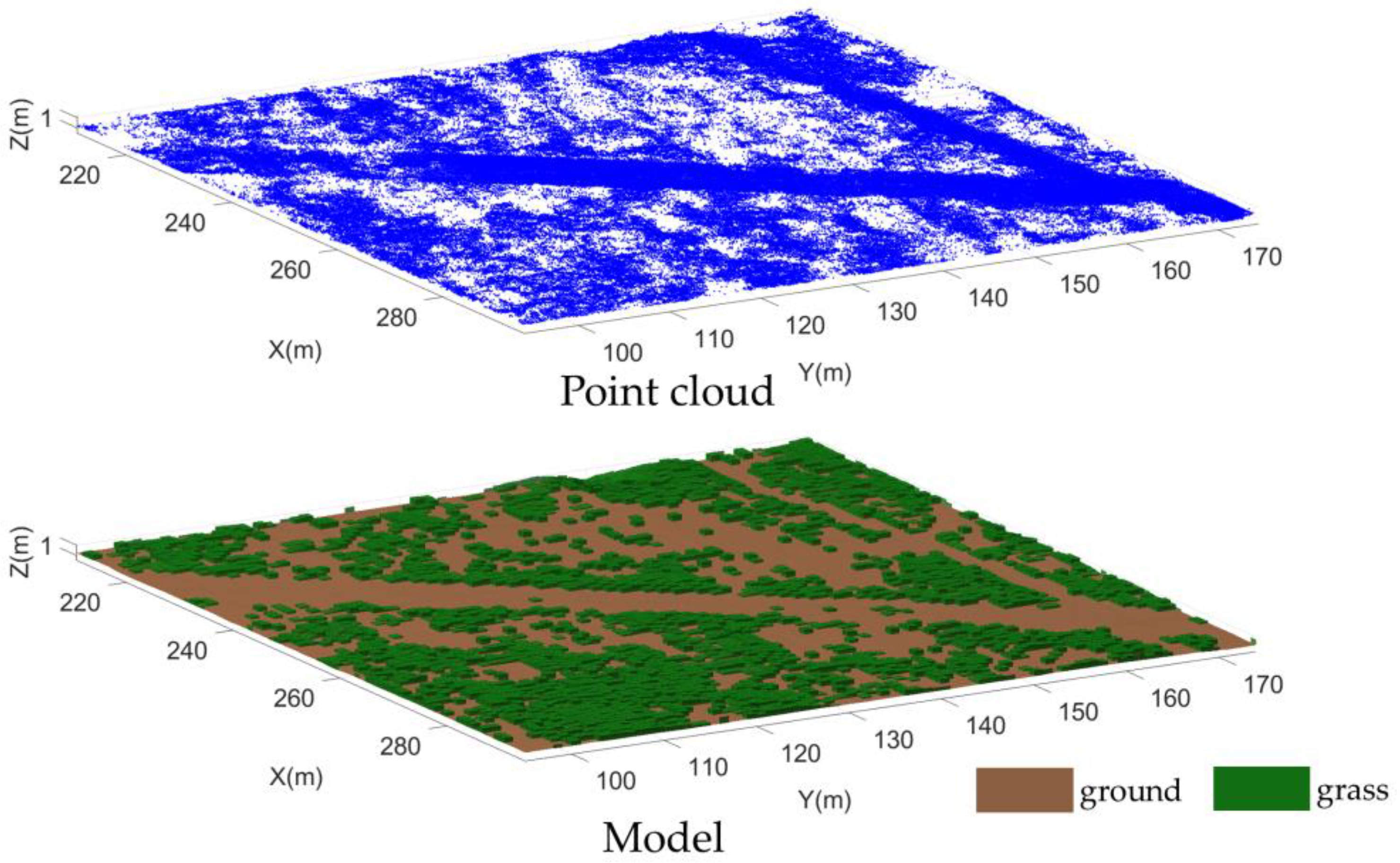
3.2. Ground–Grass Model Construction
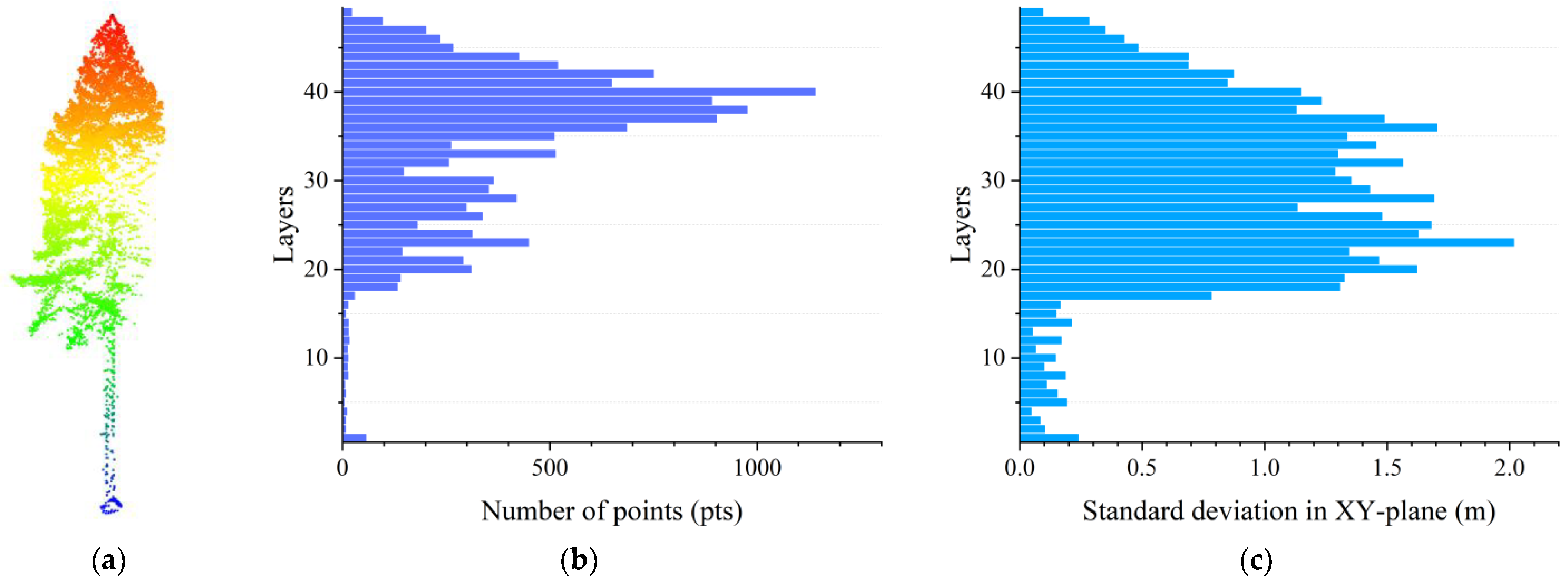
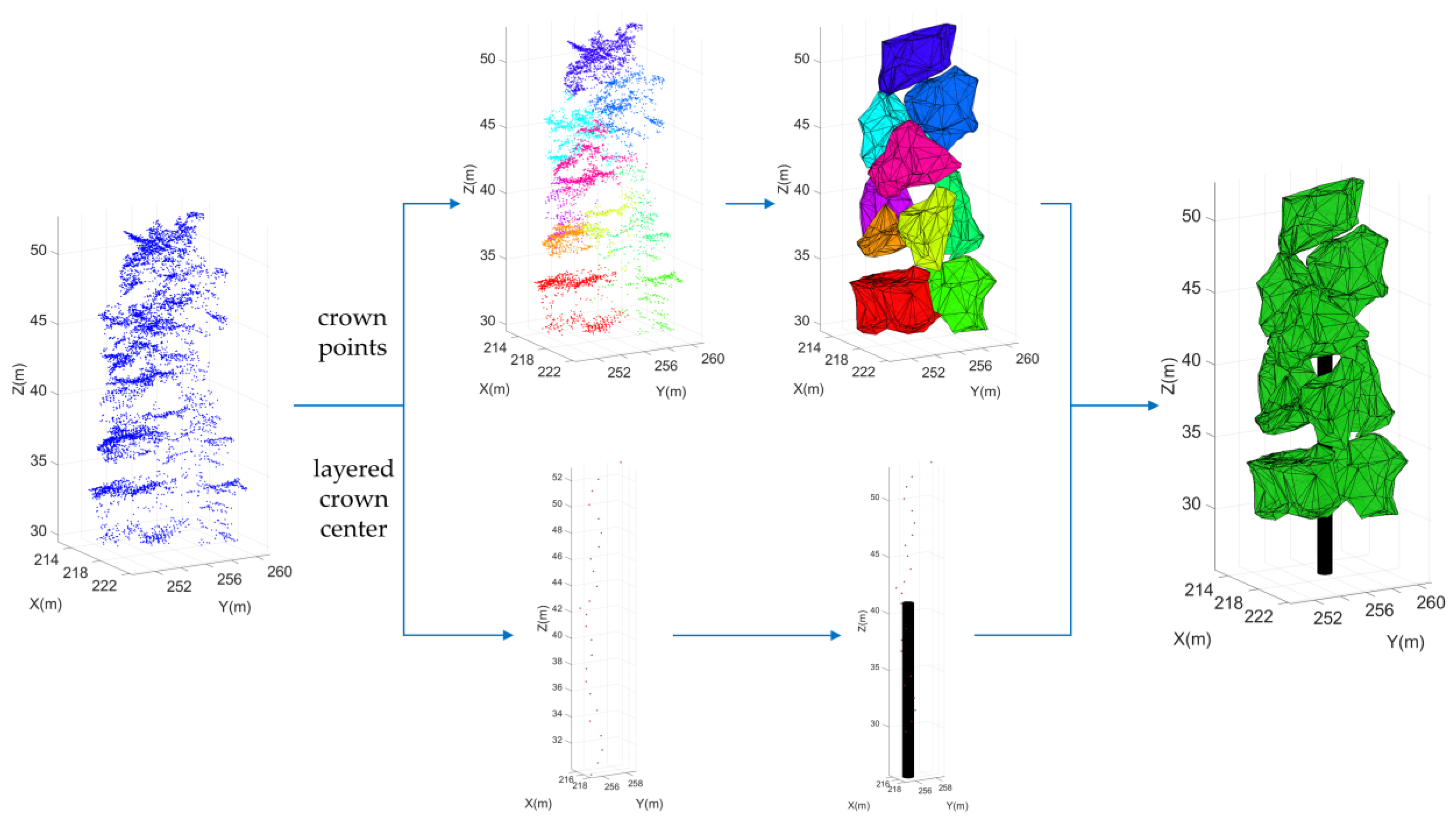
3.3. Tree Model Construction
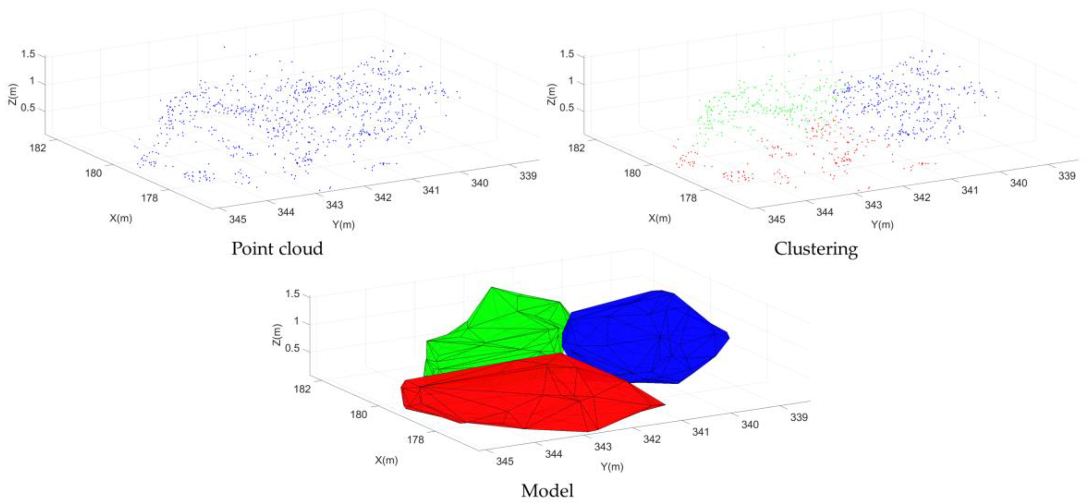
3.4. Shrub Model Construction
3.5. Forest Scene Model Construction and Accuracy Validation
4. Results and Discussion
4.1. Validation of Point Cloud Segmentation
4.2. Validation of Grass, Shrub, and Tree Models
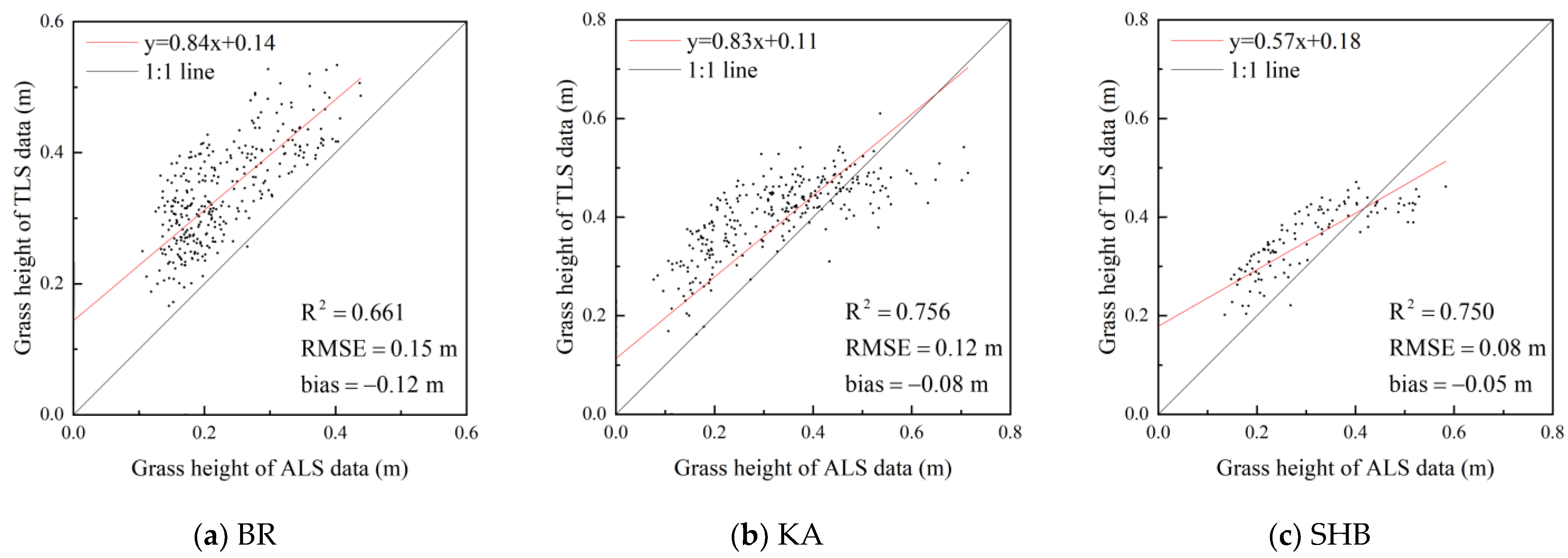
4.2.1. Validation of Grass Model
4.2.2. Validation of Shrub Model
4.2.3. Validation of Tree Model
- (1)
- Validation of Tree Position
- (2)
- Validation of Tree Height
- (3)
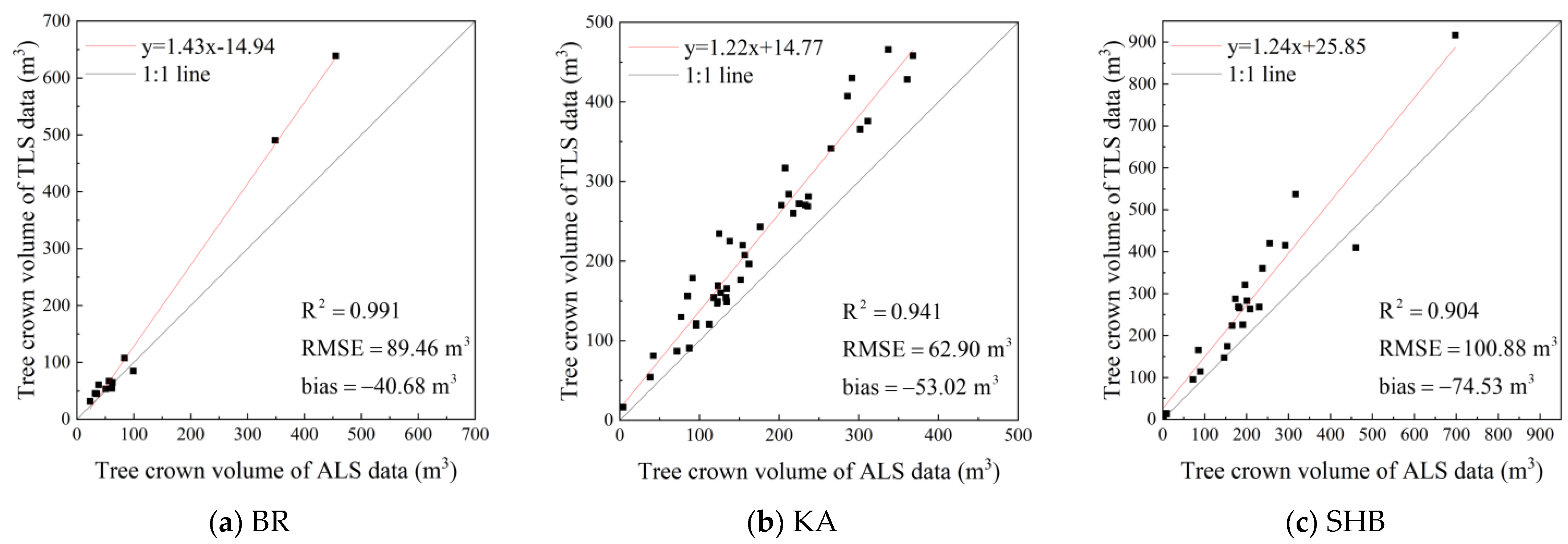
- Validation of Tree Crown Volume
4.3. Forest Scene Model Reconstruction Results
4.4. Comparison with Other Modeling Methods
5. Conclusions
Author Contributions
Funding
Data Availability Statement
Acknowledgments
Conflicts of Interest
References
- De Boissieu, F.; Heuschmidt, F.; Lauret, N.; Ebengo, D.M.; Vincent, G.; Féret, J.-B.; Yin, T.; Gastellu-Etchegorry, J.-P.; Costeraste, J.; Lefèvre-Fonollosa, M.-J.; et al. Validation of the DART Model for Airborne Laser Scanner Simulations on Complex Forest Environments. IEEE J. Sel. Top. Appl. Earth Obs. Remote Sens. 2023, 16, 8379–8394. [Google Scholar] [CrossRef]
- Wang, W.; Li, Y.; Huang, H.; Hong, L.; Du, S.; Xie, L.; Li, X.; Guo, R.; Tang, S. Branching the Limits: Robust 3D Tree Reconstruction from Incomplete Laser Point Clouds. Int. J. Appl. Earth Obs. Geoinf. 2023, 125, 103557. [Google Scholar] [CrossRef]
- Xiao, W.; Xu, S.; Elberink, S.O.; Vosselman, G. Individual Tree Crown Modeling and Change Detection from Airborne Lidar Data. IEEE J. Sel. Top. Appl. Earth Obs. Remote Sens. 2016, 9, 3467–3477. [Google Scholar] [CrossRef]
- Gastellu-Etchegorry, J.-P.; Yin, T.; Lauret, N.; Grau, E.; Rubio, J.; Cook, B.D.; Morton, D.C.; Sun, G. Simulation of Satellite, Airborne and Terrestrial LiDAR with DART (I): Waveform Simulation with Quasi-Monte Carlo Ray Tracing. Remote Sens. Environ. 2016, 184, 418–435. [Google Scholar] [CrossRef]
- Zhao, K.; Suarez, J.C.; Garcia, M.; Hu, T.; Wang, C.; Londo, A. Utility of Multitemporal Lidar for Forest and Carbon Monitoring: Tree Growth, Biomass Dynamics, and Carbon Flux. Remote Sens. Environ. 2018, 204, 883–897. [Google Scholar] [CrossRef]
- Li, J.; Wu, H.; Xiao, Z.; Lu, H. 3D Modeling of Laser-Scanned Trees Based on Skeleton Refined Extraction. Int. J. Appl. Earth Obs. Geoinf. 2022, 112, 102943. [Google Scholar] [CrossRef]
- Deng, S.; Jing, S.; Zhao, H. A Hybrid Method for Individual Tree Detection in Broadleaf Forests Based on UAV-LiDAR Data and Multistage 3D Structure Analysis. Forests 2024, 15, 1043. [Google Scholar] [CrossRef]
- Yin, T.; Cook, B.D.; Morton, D.C. Three-Dimensional Estimation of Deciduous Forest Canopy Structure and Leaf Area Using Multi-Directional, Leaf-on and Leaf-off Airborne Lidar Data. Agric. For. Meteorol. 2022, 314, 108781. [Google Scholar] [CrossRef]
- Liu, S.; Deng, Y.; Zhang, J.; Wang, J.; Duan, D. Extraction of Arbors from Terrestrial Laser Scanning Data Based on Trunk Axis Fitting. Forests 2024, 15, 1217. [Google Scholar] [CrossRef]
- Li, R.; Bu, G.; Wang, P. An Automatic Tree Skeleton Extracting Method Based on Point Cloud of Terrestrial Laser Scanner. Int. J. Opt. 2017, 2017, 5408503. [Google Scholar] [CrossRef]
- Yun, T.; Jiang, K.; Li, G.; Eichhorn, M.P.; Fan, J.; Liu, F.; Chen, B.; An, F.; Cao, L. Individual Tree Crown Segmentation from Airborne LiDAR Data Using a Novel Gaussian Filter and Energy Function Minimization-Based Approach. Remote Sens. Environ. 2021, 256, 112307. [Google Scholar] [CrossRef]
- Kukkonen, M.; Maltamo, M.; Korhonen, L.; Packalen, P. Fusion of Crown and Trunk Detections from Airborne UAS Based Laser Scanning for Small Area Forest Inventories. Int. J. Appl. Earth Obs. Geoinf. 2021, 100, 102327. [Google Scholar] [CrossRef]
- André, F.; de Wergifosse, L.; de Coligny, F.; Beudez, N.; Ligot, G.; Gauthray-Guyénet, V.; Courbaud, B.; Jonard, M. Radiative Transfer Modeling in Structurally Complex Stands: Towards a Better Understanding of Parametrization. Ann. For. Sci. 2021, 78, 1–21. [Google Scholar] [CrossRef]
- Liu, K.; Shen, X.; Cao, L.; Wang, G.; Cao, F. Estimating Forest Structural Attributes Using UAV-LiDAR Data in Ginkgo Plantations. ISPRS J. Photogramm. Remote Sens. 2018, 146, 465–482. [Google Scholar] [CrossRef]
- Yan, W.; Guan, H.; Cao, L.; Yu, Y.; Gao, S.; Lu, J. An Automated Hierarchical Approach for Three-Dimensional Segmentation of Single Trees Using UAV LiDAR Data. Remote Sens. 2018, 10, 1999. [Google Scholar] [CrossRef]
- Chang, L.; Fan, H.; Zhu, N.; Dong, Z. A Two-Stage Approach for Individual Tree Segmentation From TLS Point Clouds. IEEE J. Sel. Top. Appl. Earth Obs. Remote Sens. 2022, 15, 8682–8693. [Google Scholar] [CrossRef]
- Hu, S.; Li, Z.; Zhang, Z.; He, D.; Wimmer, M. Efficient Tree Modeling from Airborne LiDAR Point Clouds. Comput. Graph. 2017, 67, 1–13. [Google Scholar] [CrossRef]
- Kato, A.; Moskal, L.M.; Schiess, P.; Swanson, M.E.; Calhoun, D.; Stuetzle, W. Capturing Tree Crown Formation through Implicit Surface Reconstruction Using Airborne Lidar Data. Remote Sens. Environ. 2009, 113, 1148–1162. [Google Scholar] [CrossRef]
- Hu, C.; Ru, Y.; Fang, S.; Zhou, H.; Xue, J.; Zhang, Y.; Li, J.; Xu, G.; Fan, G. A Tree Point Cloud Simplification Method Based on FPFH Information Entropy. Forests 2023, 14, 1507. [Google Scholar] [CrossRef]
- Wang, S.; Hu, Q.; Xiao, D.; He, L.; Liu, R.; Xiang, B.; Kong, Q. A New Point Cloud Simplification Method with Feature and Integrity Preservation by Partition Strategy. Measurement 2022, 197, 111173. [Google Scholar] [CrossRef]
- Qi, J.; Xie, D.; Jiang, J.; Huang, H. 3D Radiative Transfer Modeling of Structurally Complex Forest Canopies through a Lightweight Boundary-Based Description of Leaf Clusters. Remote Sens. Environ. 2022, 283, 113301. [Google Scholar] [CrossRef]
- Yang, P.; van der Tol, C.; Yin, T.; Verhoef, W. The SPART Model: A Soil-Plant-Atmosphere Radiative Transfer Model for Satellite Measurements in the Solar Spectrum. Remote Sens. Environ. 2020, 247, 111870. [Google Scholar] [CrossRef]
- Pfeifer, N.; Gorte, B.; Winterhalder, D. Automatic Reconstruction of Single Trees from Terrestrial Laser Scanner Data. Remote Sens. Spat. Inf. Sci. 2004, 35, 119–124. [Google Scholar]
- Vosselman, G. 3D reconstruction of roads and trees for city modelling. Int. Arch. Photogramm., Remote Sens.Spat. Inf. Sci. 2003, 34, 231–236. [Google Scholar]
- Morsdorf, F.; Meier, E.; Kötz, B.; Itten, K.I.; Dobbertin, M.; Allgöwer, B. LIDAR-Based Geometric Reconstruction of Boreal Type Forest Stands at Single Tree Level for Forest and Wildland Fire Management. Remote Sens. Environ. 2004, 92, 353–362. [Google Scholar] [CrossRef]
- Wang, Y.; Weinacker, H.; Koch, B. A Lidar Point Cloud Based Procedure for Vertical Canopy Structure Analysis And 3D Single Tree Modelling in Forest. Sensors 2008, 8, 3938–3951. [Google Scholar] [CrossRef]
- Lin, X.; Li, A.; Bian, J.; Zhang, Z.; Lei, G.; Chen, L.; Qi, J. Reconstruction of a Large-Scale Realistic Three-Dimensional (3-D) Mountain Forest Scene for Radiative Transfer Simulations. Gisci. Remote Sens. 2023, 60, 2261993. [Google Scholar] [CrossRef]
- Li, W.; Hu, X.; Su, Y.; Tao, S.; Ma, Q.; Guo, Q. A New Method for Voxel-based Modelling of Three-dimensional Forest Scenes with Integration of Terrestrial and Airborne LIDAR Data. Methods Ecol. Evol. 2024, 15, 569–582. [Google Scholar] [CrossRef]
- Qi, J.; Xie, D.; Yin, T.; Yan, G.; Gastellu-Etchegorry, J.-P.; Li, L.; Zhang, W.; Mu, X.; Norford, L.K. LESS: LargE-Scale Remote Sensing Data and Image Simulation Framework over Heterogeneous 3D Scenes. Remote Sens. Environ. 2019, 221, 695–706. [Google Scholar] [CrossRef]
- Janoutová, R.; Homolová, L.; Malenovský, Z.; Hanuš, J.; Lauret, N.; Gastellu-Etchegorry, J.-P. Influence of 3D Spruce Tree Representation on Accuracy of Airborne and Satellite Forest Reflectance Simulated in DART. Forests 2019, 10, 292. [Google Scholar] [CrossRef]
- Jarron, L.R.; Coops, N.C.; MacKenzie, W.H.; Tompalski, P.; Dykstra, P. Detection of Sub-Canopy Forest Structure Using Airborne LiDAR. Remote Sens. Environ. 2020, 244, 111770. [Google Scholar] [CrossRef]
- Wing, B.M.; Ritchie, M.W.; Boston, K.; Cohen, W.B.; Gitelman, A.; Olsen, M.J. Prediction of understory vegetation cover with airborne lidar in an interior ponderosa pine forest. Remote Sens. Environ. 2012, 124, 730–741. [Google Scholar] [CrossRef]
- Weiser, H.; Schäfer, J.; Winiwarter, L.; Krašovec, N.; Fassnacht, F.E.; Höfle, B. Individual Tree Point Clouds and Tree Measurements from Multi-Platform Laser Scanning in German Forests. Earth Syst. Sci. Data 2022, 14, 2989–3012. [Google Scholar] [CrossRef]
- Zhao, X.; Qi, J.; Yu, Z.; Yuan, L.; Huang, H. Fine-Scale Quantification of Absorbed Photosynthetically Active Radiation (APAR) in Plantation Forests with 3D Radiative Transfer Modeling and LiDAR Data. Plant Phenomics 2024, 6, 0166. [Google Scholar] [CrossRef]
- Tusa, E.; Monnet, J.-M.; Barré, J.-B.; Mura, M.D.; Dalponte, M.; Chanussot, J. Individual Tree Segmentation Based on Mean Shift and Crown Shape Model for Temperate Forest. IEEE Geosci. Remote Sens. Lett. 2021, 18, 2052–2056. [Google Scholar] [CrossRef]
- Zhang, W.; Qi, J.; Wan, P.; Wang, H.; Xie, D.; Wang, X.; Yan, G. An Easy-to-Use Airborne LiDAR Data Filtering Method Based on Cloth Simulation. Remote Sens. 2016, 8, 501. [Google Scholar] [CrossRef]
- Fischler, M.A.; Bolles, R.C. Random Sample Consensus: A Paradigm for Model Fitting with Applications to Image Analysis and Automated Cartography. Commun. ACM 1981, 24, 381–395. [Google Scholar] [CrossRef]
- Wang, X.; Zhang, Y.; Luo, Z. Combining Trunk Detection with Canopy Segmentation to Delineate Single Deciduous Trees Using Airborne LiDAR Data. IEEE Access 2020, 8, 99783–99796. [Google Scholar] [CrossRef]
- Zhou, X.; Alexiou, E.; Viola, I.; Cesar, P. PointPCA+: Extending PointPCA Objective Quality Assessment Metric. In Proceedings of the IEEE International Conference on Image Processing Challenges and Workshops (ICIPCW), Kuala Lumpur, Malaysia, 8–11 October 2023. [Google Scholar] [CrossRef]
- Comaniciu, D.; Meer, P. Mean Shift: A Robust Approach toward Feature Space Analysis. IEEE Trans. Pattern Anal. Mach. Intell. 2002, 24, 603–619. [Google Scholar] [CrossRef]
- Goutte, C.; Gaussier, E. A Probabilistic Interpretation of Precision, Recall and F-Score, with Implication for Evaluation. In Proceedings of the 27th European Conference on Advances in Information Retrieval Research, Santiago de Compostela, Spain, 21–23 March 2005. [Google Scholar] [CrossRef]
- Wang, J.; Chen, X.; Cao, L.; An, F.; Chen, B.; Xue, L.; Yun, T. Individual Rubber Tree Segmentation Based on Ground-Based LiDAR Data and Faster R-CNN of Deep Learning. Forests 2019, 10, 793. [Google Scholar] [CrossRef]
- Chen, X.; Jiang, K.; Zhu, Y.; Wang, X.; Yun, T. Individual Tree Crown Segmentation Directly from UAV-Borne LiDAR Data Using the PointNet of Deep Learning. Forests 2021, 12, 131. [Google Scholar] [CrossRef]
- Xi, Z.; Hopkinson, C. 3D Graph-Based Individual-Tree Isolation (Treeiso) from Terrestrial Laser Scanning Point Clouds. Remote Sens. 2022, 14, 6116. [Google Scholar] [CrossRef]
- Xiang, B.; Wielgosz, M.; Kontogianni, T.; Peters, T.; Puliti, S.; Astrup, R.; Schindler, K. Automated Forest Inventory: Analysis of High-Density Airborne LiDAR Point Clouds with 3D Deep Learning. Remote Sens. Environ. 2024, 305, 114078. [Google Scholar] [CrossRef]


| Sample Plots | Location | Plot Size | Average Slope (°) | Forest Type | Average Tree Height (m) | Vegetation Coverage |
|---|---|---|---|---|---|---|
| BR | 49.01° N, 8.69° E | 300 × 300 m | 21.80 | Mixed Broadleaf–Conifer Forest | 14.0 | 80.53% |
| KA | 49.03° N, 8.43° E | 300 × 300 m | 9.09 | Mixed Broadleaf–Conifer Forest | 20.2 | 91.76% |
| SHB | 42.42° N, 117.31° E | 300 × 300 m | 9.09 | Coniferous Forest | 17.7 | 88.45% |
| DZ | 24.32° N, 102.57° E | 300 × 170 m | 10.21 | Mixed Broadleaf–Conifer Forest | 11.6 | 82.36% |
| GX | 25.45° N, 110.46° E | 300 × 340 m | 5.79 | Broad-leaved Forest | 12.2 | 71.66% |
| SL | 27.62° N, 99.74° E | 210 × 200 m | 17.68 | Coniferous Forest | 12.1 | 81.74% |
| Sample Plots | Acquisition Time | Acquisition Equipment | Flight Altitude (m) | Pulse Repetition Frequency (kHz) | Elevation Accuracy (mm) | Density (pts/m2) |
|---|---|---|---|---|---|---|
| BR | 5 July 2019 | RIEGL VQ-780i | 650 | 1000 | 20 | 27 |
| KA | 5 July 2019 | RIEGL VQ-780i | 650 | 1000 | 20 | 26 |
| SHB | 21 July 2022 | RIEGL VUX-1UAV | 60 | 550 | 10 | 108 |
| DZ | 5 June 2022 | RIEGL VUX-1UAV | 70 | 550 | 10 | 139 |
| GX | 11 October 2021 | RIEGL VUX-1UAV | 70 | 550 | 10 | 74 |
| SL | 25 May 2021 | RIEGL VUX-1UAV | 60 | 550 | 10 | 129 |
| Sample Plots | Number of Individual Trees | Number of Trunk Positions | Number of Shrub Point Cloud Clusters | |
|---|---|---|---|---|
| ALS | BR | 38 | / | / |
| KA | 51 | / | / | |
| SHB | 48 | / | / | |
| DZ | 45 | / | / | |
| GX | 57 | / | / | |
| SL | 53 | / | / | |
| TLS | BR | 28 | 28 | 11 |
| KA | 30 | 30 | 16 | |
| SHB | 50 | 50 | 11 | |
| DZ | 40 | 40 | 18 | |
| GX | 53 | 53 | 17 | |
| SL | 44 | 44 | 10 |
| Method | Sample Plots | Number of Actual Trees | Number of Segmented Trees | TP | FN | FP | r (%) | p (%) | f (%) |
|---|---|---|---|---|---|---|---|---|---|
| treeiso | BR | 38 | 41 | 29 | 9 | 12 | 76.31 | 70.73 | 73.42 |
| KA | 51 | 53 | 40 | 11 | 13 | 78.43 | 75.41 | 76.92 | |
| SHB | 48 | 50 | 42 | 6 | 8 | 87.50 | 84.00 | 85.71 | |
| DZ | 45 | 43 | 33 | 12 | 10 | 73.33 | 76.74 | 75.00 | |
| GX | 57 | 52 | 43 | 14 | 9 | 75.44 | 82.69 | 78.90 | |
| SL | 53 | 57 | 43 | 10 | 14 | 81.13 | 75.44 | 78.18 | |
| ForAINet | BR | 38 | 36 | 30 | 8 | 6 | 78.95 | 83.33 | 81.08 |
| KA | 51 | 47 | 42 | 9 | 5 | 82.35 | 89.36 | 85.71 | |
| SHB | 48 | 46 | 45 | 3 | 1 | 93.75 | 97.83 | 95.94 | |
| DZ | 45 | 45 | 38 | 7 | 7 | 84.44 | 84.44 | 84.44 | |
| GX | 57 | 55 | 47 | 10 | 8 | 82.46 | 85.45 | 83.93 | |
| SL | 53 | 57 | 48 | 5 | 9 | 90.57 | 84.21 | 87.27 | |
| Proposed | BR | 38 | 33 | 31 | 7 | 2 | 81.58 | 93.94 | 87.32 |
| KA | 51 | 48 | 44 | 7 | 4 | 86.27 | 91.67 | 88.89 | |
| SHB | 48 | 46 | 44 | 4 | 2 | 91.67 | 95.65 | 93.62 | |
| DZ | 45 | 47 | 41 | 4 | 6 | 91.11 | 87.23 | 89.13 | |
| GX | 57 | 53 | 50 | 7 | 3 | 87.72 | 94.34 | 90.91 | |
| SL | 53 | 56 | 49 | 4 | 7 | 92.45 | 87.50 | 89.91 |
| Sample Plots | BR | KA | SHB | DZ | GX | SL |
|---|---|---|---|---|---|---|
| Number of actual shrubs | 11 | 16 | 11 | 18 | 17 | 10 |
| Number of segmented shrubs | 8 | 12 | 10 | 12 | 14 | 6 |
| Extraction accuracy | 72.73% | 75.00% | 90.91% | 66.67% | 82.35% | 60.00% |
| Sample Plots | Number of Trees | Our Method | Center of Crown Projection | ||||
|---|---|---|---|---|---|---|---|
| (m) | (m) | (m) | (m) | (m) | (m) | ||
| BR | 28 | 0.19 | 0.29 | 0.37 | 0.58 | 0.45 | 0.79 |
| KA | 30 | 0.23 | 0.20 | 0.33 | 0.67 | 0.72 | 1.09 |
| SHB | 50 | 0.26 | 0.25 | 0.41 | 0.63 | 0.66 | 1.01 |
| DZ | 30 | 0.22 | 0.24 | 0.33 | 0.49 | 0.41 | 0.64 |
| GX | 32 | 0.25 | 0.29 | 0.38 | 0.72 | 0.40 | 0.82 |
| SL | 49 | 0.28 | 0.23 | 0.36 | 0.58 | 0.38 | 0.69 |
| Total | 219 | 0.24 | 0.25 | 0.35 | 0.61 | 0.50 | 0.80 |
| Sample Plots | Tree Volume Proportion | Shrub Volume Proportion | Grass Volume Proportion | Total Vegetation Volume (m3) |
|---|---|---|---|---|
| BR | 92.21% | 7.72% | 0.07% | 574,702.62 |
| KA | 85.96% | 13.80% | 0.24% | 687,645.62 |
| SHB | 97.04% | 2.89% | 0.07% | 568,656.26 |
| DZ | 93.16% | 6.49% | 0.35% | 424,956.25 |
| GX | 91.36% | 6.25% | 2.39% | 557,095.37 |
| SL | 93.03% | 6.84% | 0.13% | 389,406.25 |
| Original Point Cloud | Simplified Point Cloud | Voxel Model (1 m) | Voxel Model (0.5 m) | Proposed Model | |
|---|---|---|---|---|---|
| coniferous tree |  | 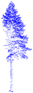 |  | 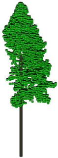 | 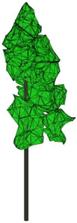 |
| broadleaf trees | 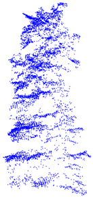 |  | 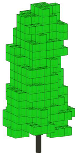 | 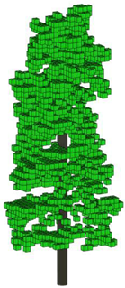 | 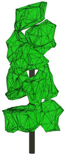 |
| Sample Plots | Original Point Cloud | Simplified Point Cloud | Voxel Model at Different Resolutions | Our Model | |
|---|---|---|---|---|---|
| 1 m | 0.5 m | ||||
| BR | 451 MB | 143 MB | 155 MB | 584 MB | 98 MB |
| KA | 551 MB | 211 MB | 177 MB | 681 MB | 119 MB |
| SHB | 1.03 GB | 153 MB | 172 MB | 719 MB | 204 MB |
| DZ | 789 MB | 55 MB | 85 MB | 326 MB | 107 MB |
| GX | 715 MB | 91 MB | 138 MB | 598 MB | 156 MB |
| SL | 562 MB | 44 MB | 55 MB | 219 MB | 102 MB |
Disclaimer/Publisher’s Note: The statements, opinions and data contained in all publications are solely those of the individual author(s) and contributor(s) and not of MDPI and/or the editor(s). MDPI and/or the editor(s) disclaim responsibility for any injury to people or property resulting from any ideas, methods, instructions or products referred to in the content. |
© 2024 by the authors. Licensee MDPI, Basel, Switzerland. This article is an open access article distributed under the terms and conditions of the Creative Commons Attribution (CC BY) license (https://creativecommons.org/licenses/by/4.0/).
Share and Cite
Xu, D.; Yang, X.; Wang, C.; Xi, X.; Fan, G. Three-Dimensional Reconstruction of Forest Scenes with Tree–Shrub–Grass Structure Using Airborne LiDAR Point Cloud. Forests 2024, 15, 1627. https://doi.org/10.3390/f15091627
Xu D, Yang X, Wang C, Xi X, Fan G. Three-Dimensional Reconstruction of Forest Scenes with Tree–Shrub–Grass Structure Using Airborne LiDAR Point Cloud. Forests. 2024; 15(9):1627. https://doi.org/10.3390/f15091627
Chicago/Turabian StyleXu, Duo, Xuebo Yang, Cheng Wang, Xiaohuan Xi, and Gaofeng Fan. 2024. "Three-Dimensional Reconstruction of Forest Scenes with Tree–Shrub–Grass Structure Using Airborne LiDAR Point Cloud" Forests 15, no. 9: 1627. https://doi.org/10.3390/f15091627