Forest Canopy Height Estimation Combining Dual-Polarization PolSAR and Spaceborne LiDAR Data

Abstract

Forest canopy height data are fundamental parameters of forest structure and are critical for understanding terrestrial carbon stock, global carbon cycle dynamics and forest productivity. To address the limitations of retrieving forest canopy height using conventional PolInSAR-based methods, we proposed a method to estimate forest height by combining single-temporal polarimetric synthetic aperture radar (PolSAR) images with sparse spaceborne LiDAR (forest height) measurements. The core idea of our method is that volume scattering energy variations which are linked to forest canopy height occur during radar acquisition. Specifically, our methodology begins by employing a semi-empirical inversion model directly derived from the random volume over ground (RVoG) formulation to establish the relationship between forest canopy height, volume scattering energy and wave extinction. Subsequently, PolSAR decomposition techniques are used to extract canopy volume scattering energy. Additionally, machine learning is employed to generate a spatially continuous extinction coefficient product, utilizing sparse LiDAR samples for assistance. Finally, with the derived inversion model and the resulting model parameters (i.e., volume scattering power and extinction coefficient), forest canopy height can be estimated. The performance of the proposed forest height inversion method is illustrated with L-band NASA/JPL UAVSAR from AfriSAR data conducted over the Gabon Lope National Park and airborne LiDAR data. Compared to high-accuracy airborne LiDAR data, the obtained forest canopy height from the proposed approach exhibited higher accuracy (R² = 0.92, RMSE = 6.09 m). The results demonstrate the potential and merit of the synergistic combination of PolSAR (volume scattering power) and sparse LiDAR (forest height) measurements for forest height estimation. Additionally, our approach achieves good performance in forest height estimation, with accuracy comparable to that of the multi-baseline PolInSAR-based inversion method (RMSE = 5.80 m), surpassing traditional PolSAR-based methods with an accuracy of 10.86 m. Given the simplicity and efficiency of the proposed method, it has the potential for large-scale forest height estimation applications when only single-temporal dual-polarization acquisitions are available.

1. Introduction

Forest height is one important aspect of basic forest structural data and plays a crucial role in monitoring forest natural resources, measuring terrestrial carbon storage and modeling global carbon cycle dynamics [1,2]. Over the past few decades, a range of remote sensing techniques, such as light detection and ranging (LiDAR) [3,4], optical remote sensing [5,6,7], interferometric synthetic aperture radar (InSAR) and polarimetric InSAR (PolInSAR) [8,9], have been extensively employed to map forest height globally or regionally. In the realm of these techniques, PolInSAR has been proven to be a reliable and effective technique for estimating forest canopy height over large coverage areas at a fine spatial scale for a variety of forest types and microwave bands (e.g., X-, L- and P-band) from either airborne or spaceborne platforms. This is because PolInSAR imaging systems are based on the coherent combination of polarimetric SAR (PolSAR) and InSAR imaging systems; the interferometric measurements are sensitive to both forest vertical structure (interferometric information) and physical characteristics (polarimetric information) of the scattering media.

To estimate forest height using PolInSAR data, most approaches aim to isolate the ground and canopy scattering contributions through polarimetry and measure their locations or distributions along the vertical dimension using interferometry. For this, one widely used strategy involves employing complex interferometric coherences as observables and utilizing forward coherent scattering models (e.g., random volume over ground (RVoG), two-level model (TLM) [10,11]) to establish the relationship between the PolInSAR observations and the forest parameters [12], such as canopy height and density. By performing model inversion, the forest canopy height can subsequently be retrieved.

Nevertheless, this technique also presents two limitations in its application. In first place, the approach relies on the use of the complex interferometric coherences as observables, which can be limited by various decorrelation errors, such as temporal decorrelation and geometric decorrelation [13,14]. These errors can degrade the quality of the interferograms, thereby constraining the effectiveness of PolInSAR parameter inversion. Besides the challenges associated with non-volume decorrelation affecting the performance of PolInSAR modeling, current applications of PolInSAR are constrained by the limited availability of spaceborne PolInSAR data [15]. This could be the primary reason why this approach has usually been validated with airborne PolInSAR data, but rarely with spaceborne data. In second place, height inversion with the InSAR technique relies on the sensitivity of InSAR measurements or the interferometric baseline [16,17]. Although some spaceborne SAR systems, such as ALOS-2 PALSAR, RADARSAT-2, Sentinel-1 and COSMO-SkyMed missions, have a short temporal baseline and can collect polarimetric images over forested areas, their short spatial baselines make these systems insufficiently sensitive to variation in forest canopy height. As a result, the collected PolInSAR data do not directly enable the derivation of high-accuracy forest height products.

One general solution to address these limitations has been to decrease the reliance on interferometric data, as proposed with the use of PolSAR data and empirical models, which established the relationship between polarimetric information and forest biophysical parameters (e.g., forest canopy height). In principle, if the polarimetric information or SAR parameters can provide sufficient sensitivity to forest structure, the established empirical model can directly be utilized to invert polarimetric observations into forest height. However, it is noteworthy that to enable the retrieval of forest height using that approach, the empirical model should be combined with other data sources that provide forest canopy height such as LiDAR. To this aim, Garestier et al. [18] established a pseudolinear correlation between polarimetric anisotropy and mean tree height, demonstrating that SAR polarimetry constitutes a promising tool for forest parameter retrieval at the low frequency of the P-band. In addition, there have been several efforts recently devoted to finding a more feasible forest height modeling technique by merging LiDAR and SAR components, including SAR backscatter and polarimetric parameters, with the application of machine learning [19,20,21]. These approaches involve using SAR to extrapolate LiDAR measurements and estimate forest canopy height at a large scale, where machine learning is adopted to establish the complex correlation between SAR characteristics and LiDAR measurements. Although their results are significant and show the potential of the approach for high-accuracy forest height estimation in the absence of interferometric observations, these studies focus solely on the mathematic relationship between LiDAR measurements and SAR characteristics during machine learning model training, often overlooking the physical meaning of them.

Following this investigation line, this study aims to develop a new method for forest height estimation by combining a single PolSAR image with sparse LiDAR (forest height) measurements. The main objectives of this study are as follows: (1) to derive a simplified forest height inversion model from the random volume over ground (RVoG) model [10,22]; (2) to propose a new forest height estimation framework that integrates an RVoG-based semi-empirical inversion model with machine learning by merging LiDAR and PolSAR components. Additionally, to accomplish the aforementioned objectives, the availability of LiDAR forest height data is essential. For this purpose, this study utilizes forest height measurements obtained from the ICESat-2 ATL08 data product, due to its extensive coverage of Earth’s land surface [23].

The rest of this paper is organized as follows: The proposed methodology is described in Section 2. In Section 3, the study area and available experimental datasets are described. The results obtained are summarized in Section 4. A discussion and the conclusions of this paper are outlined in Section 5 and Section 6, respectively.

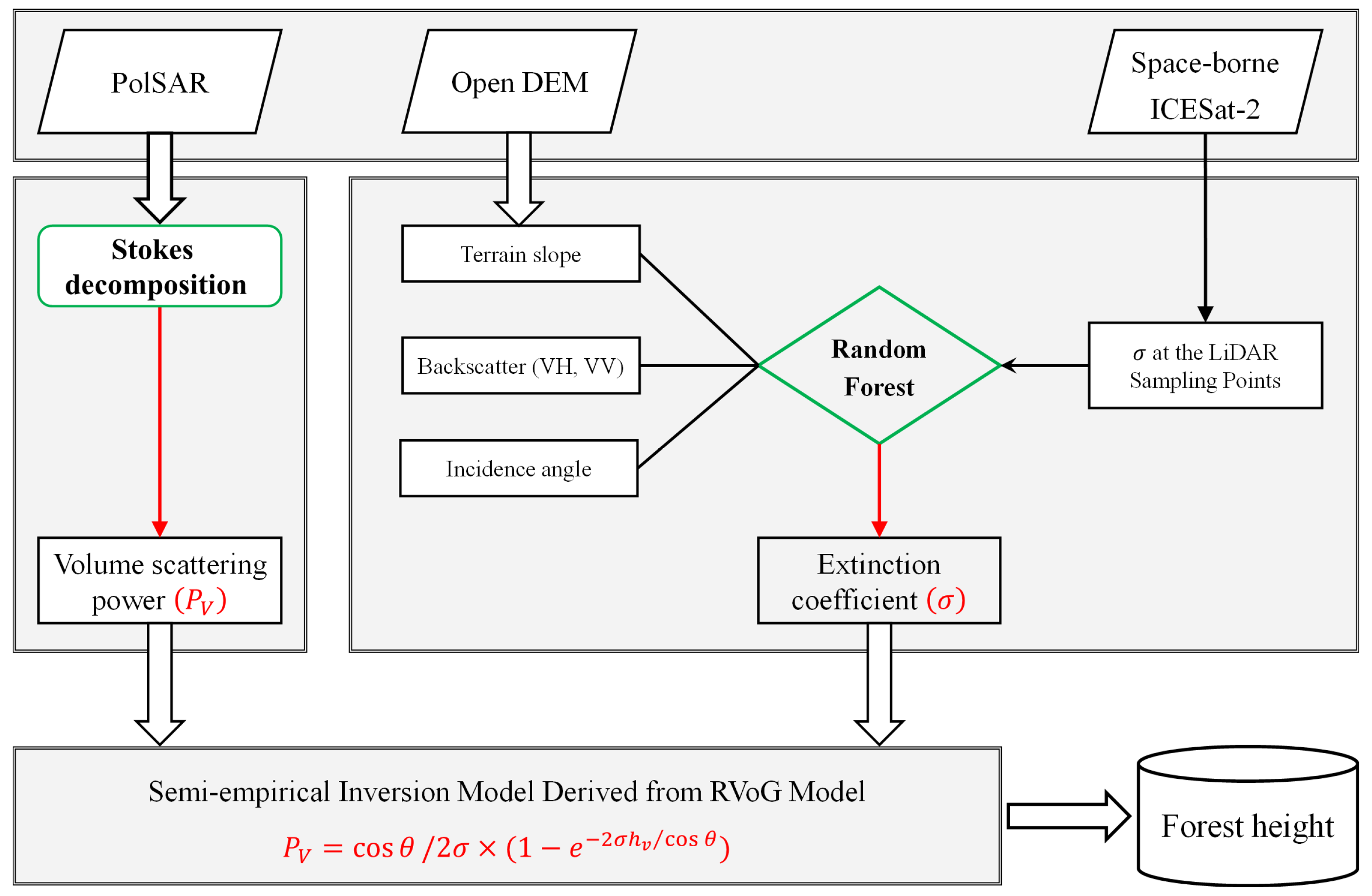
2. Methods

2.1. Semi-Empirical Inversion Model Derived from RVoG Model

The RVoG model, which considers the vegetation scene as a volume layer with randomly oriented particles over an impenetrable ground surface [10,12,24], is a well-established coherent scattering model and has been widely used for the extraction of forest physical parameters using InSAR and PolInSAR data. In this coherent scattering model, the vegetation volume can be entirely defined by two “biophysical” parameters: the top height of forest volume $h_v$ and the mean extinction coefficient $\sigma$. Inversing the RVoG model using a single-baseline acquisition typically requires fully polarimetric interferometric data and the assumption that the ground-to-volume amplitude ration is zero in at least one polarization [22]. However, few spaceborne SAR systems have the capability to collect quad-polarimetric interferometric data, while many more operational spaceborne SAR systems provide only dual-polarization data. Additionally, the performance of inversion can be impacted and distributed by the quality of the interferograms or decorrelation errors, such as the presence of temporal decorrelation [25]. Therefore, it becomes necessary to explore the inversion of forest height using as little interferometric information as possible.

One general solution is to use single-temporal PolSAR imaging for parameter inversion. Hence, the starting point is to define the coherent scattering vector observable information of a single fully polarimetric SAR image in the 3-D Pauli scattering vectors $\overrightarrow{k}$, given by

$$k={\displaystyle \frac{1}{\sqrt{2}}}\left[S_{HH}+S_{VV},S_{HH}-S_{VV},2S_{HV}\right]$$

(1)

where $S_{tr}$ stands for the complex scattering amplitude, and the subscripts represent the combination of the transmit $\left(t\right)$ and receive $\left(r\right)$ polarizations in the HV–polarimetric basis. The complete information measured by the PolSAR system can be represented in the form of one 3 × 3 coherency matrix $T$ formed using the outer product of $k$ as follows:

$$T=\langle k\cdot k^{†}\rangle$$

(2)

where $†$ combines the complex conjugate and the transpose operators. Under the RVoG model framework [12,22], the coherency matrix $T$ can be modeled as the contribution of two scattering mechanisms: ground surface and volume scatterings. Thereby, Equation (2) can be expressed by

$$T=I^V+e^{(-2\sigma h_v)/\cos \theta }{I}^G$$

(3)

where $\theta$ represents the incidence angle, and $\sigma$ is the one-way mean extinction coefficient. $I^V$ and $I^G$ stand for the integration of volume and ground scatterings, respectively, which can be expressed in terms of the forest height $\left(h_v\right)$, the mean extinction coefficient $\left(\sigma \right)$ and the incidence angle $\left(\theta \right)$, as follows [26]:

$$\begin{array}{l}{I}^V=e^{\left(-2\sigma h_v\right)/\cos \theta }{\displaystyle {\int }_0^{h_v}{e}^{\left(2\sigma z^{\prime }\right)/\cos \theta }{T}_{V}d{z}^{\prime }}={\displaystyle \frac{\cos \theta }{2\sigma }}\left(1-e^{\left(-2\sigma h_v\right)/\cos \theta }\right)T_V\\ I^G={\displaystyle {\int }_0^{h_v}\delta \left(z^{\prime }\right)e^{\left(2\sigma z^{\prime }\right)/\cos \theta }{T}_{g}d{z}^{\prime }=T_g}\end{array}$$

(4)

The second way involves signal separation techniques, which is equivalent to increasing the number of observables. Among these techniques, a commonly used method is based on polarimetric decomposition. Specifically, from the perspective of the polarimetric decomposition, the coherency matrix T can be modeled as the sum of the powers of multiple scattering mechanisms. According to the assumption of the RVoG mode, Equation (2) can be expressed as follows [27]:

$$T=P_V{T}_V+P_g{T}_g$$

(5)

where $P_V$ and $P_g$ correspond to the power from the volume and ground scattering mechanisms, respectively. By combining Equations (3)–(5), the following expression can be derived:

$${\displaystyle \frac{\cos \theta }{2\sigma }}\left(1-e^{\left(-2\sigma h_v\right)/\cos \theta }\right)T_V+e^{(-2\sigma h_v)/\cos \theta }{T}_g=P_V{T}_V+P_g{T}_g$$

(6)

Subsequently, by ignoring the second term in Equation (6), i.e., ground scattering contribution, a semi-empirical inversion model is derived and represented, as shown in Equation (7):

$$P_V={\displaystyle \frac{\cos \theta }{2\sigma }}\left(1-e^{\left(-2\sigma h_v\right)/\cos \theta }\right)$$

(7)

As stated earlier, it is assumed that variations in volume height primarily result from the changes in volume scattering power. In such a way, forest height can be estimated based on the volume scattering power. However, before estimating the forest height for the entire SAR scene via Equation (7), both the volume scattering power and the mean extinction coefficient still remain unknown. To address this issue, this study proposes a specialized data processing solution, which is detailed in Section 2.2.

2.2. Parameter Extraction

2.2.1. Volume Scattering Power Extraction Based on Stokes Decomposition

To accommodate the demands of most spaceborne polarimetric SAR systems that provide only dual-pol data, such as JAXA’s ALOS-PALSAR and ESA’s Sentinel-1, this study adopted the generalized Stokes decomposition method based on dual-polarization SAR data, as proposed by [28], to retrieve the volume scattering power. The corresponding data processing comprises three main steps:

(1) Data Preprocessing

For the conventional dual-polarization SAR system, the collected target scattering matrix can be represented by a two-element complex vector $S$, as follows:

$$S=\left[\begin{array}{c}{S}_{XH}\\ S_{XV}\end{array}\right]$$

(8)

where the subscript $X$ represents the transmit polarization, which can be either linear H or V in the HV–polarimetric basis. Based on the lexicographic basis, a cross-correlation matrix of $C_2$ with either an HH-HV or VV-VH dual-polarization combination is formed as follows [29]:

$$C_2=\left[\begin{array}{cc}{\left|S_{HH}\right|}^2& S_{HH}{S}_{HV}^{\ast }\\ S_{HH}^{\ast }{S}_{HV}& {\left|S_{HV}\right|}^2\end{array}\right] \mathrm{or} C_2=\left[\begin{array}{cc}{\left|S_{VV}\right|}^2& S_{VV}{S}_{VH}^{\ast }\\ S_{VV}^{\ast }{S}_{VH}& {\left|S_{VH}\right|}^2\end{array}\right]$$

(9)

These relationships can then be used to extend a scattering power decomposition algorithm to dual-polarization data.

(2) Generalized Stokes Vector Decomposition

To achieve this goal, the observed Stokes vector can be modeled as a sum of three components, as follows:

$$S=m_v{S}_v+m_p{S}_p+m_n{S}_n$$

(10)

where the first term $\left(m_v{S}_v\right)$ indicates the contribution from volume scattering, the second term $\left(m_p{S}_p\right)$ represents the components of the fully polarized wave, while the last term $\left(m_n{S}_n\right)$ indicates the noise term that can be effectively reduced by data processing (e.g., multi-looking or speckle filtering). Therefore, the equation for $S_p$ and $S_v$ can be obtained as follows [28]:

$$S_p^{T}G{S}_p={(S-m_v{S}_v)}^{T}G(S-m_v{S}_v)=0$$

(11)

where G is a family of matrices commonly employed in the Stokes algebra [22], as shown in the following:

$$G=\left[\begin{array}{cccc}1& 0& 0& 0\\ 0& -1& 0& 0\\ 0& 0& -1& 0\\ 0& 0& 0& -1\end{array}\right]$$

(12)

In addition, it is noteworthy that since the volume Stokes vector is related to the polarization states, different dual-polarization configurations correspond to different dual-polarization Stokes vectors. Specifically, for the HH-HV polarization combination, the corresponding volume Stokes vector is $S_v={\left[\begin{array}{cccc}1& 1/2& 0& 0\end{array}\right]}^T$. In the case of the VV-VH polarization combination, the associated Stokes vector is $S_v={\left[\begin{array}{cccc}1& -1/2& 0& 0\end{array}\right]}^T$.

(3) Volume Scattering Power Retrieval

By substituting $S_v$ and $G$ of Equation (11) with their respective vectors, a quadratic equation in one variable can be obtained as follows:

$$a{m}_v^2+b{m}_v+c=0$$

(13)

Finally, according to energy conservation $\left(m_v\le \le S_1\right)$, only one root of this quadratic provides a unique solution for the volume scattering power.

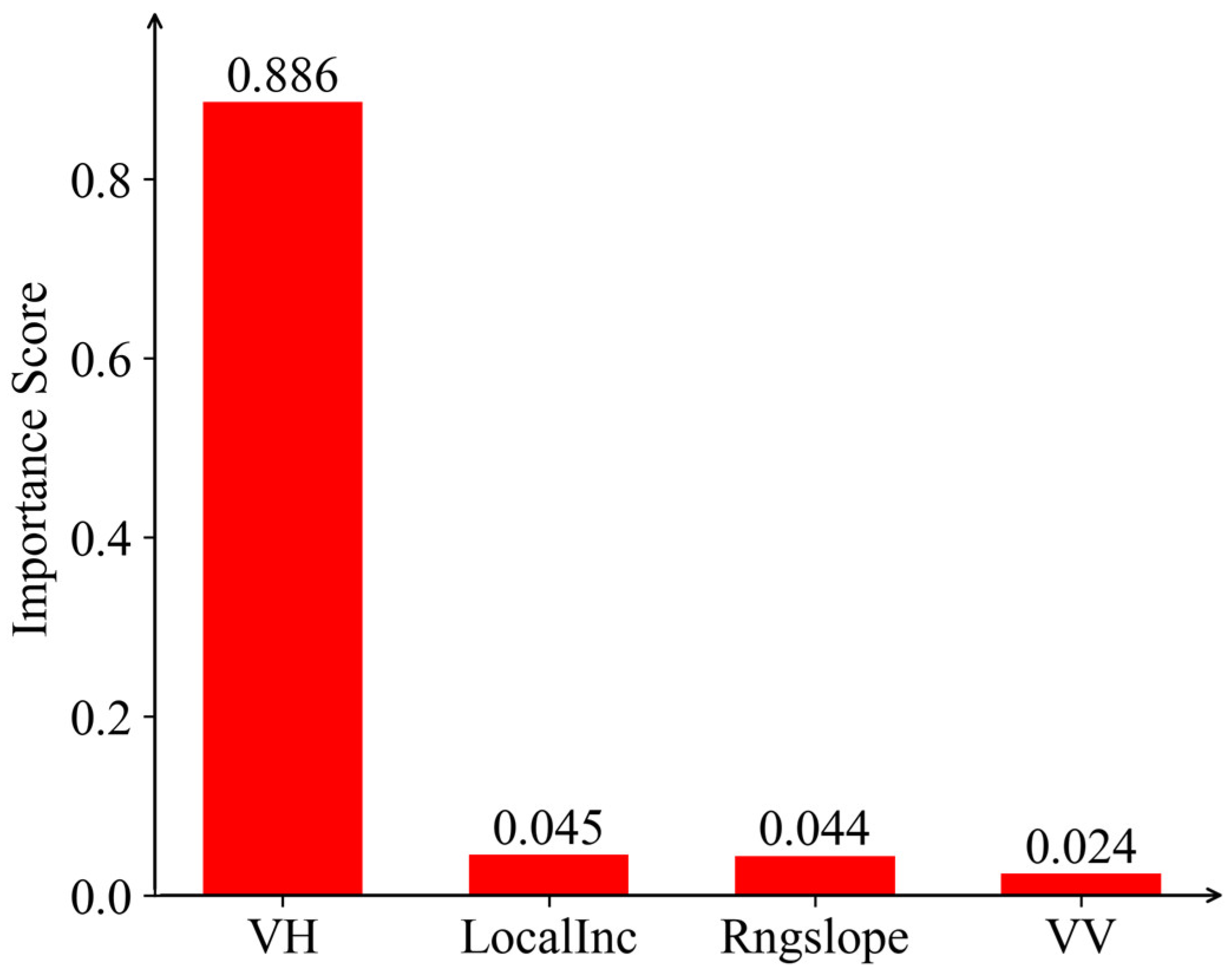
2.2.2. Extinction Coefficient Estimation Based on Machine Learning

Once the volume scattering power is determined by solving Equation (13), the extinction coefficient $\left(\sigma \right)$ remains the only unknown parameter in Equation (7) for the forest height estimation. From Equation (7), it appears that the extinction coefficient controls the rate of variation in the volume scattering power as a function of volume height. While previous studies have suggested that extinction accounts for the combined effects of the absorption of energy by volume and scattering loss due to the presence of scattering particles [22,30], in practice, numerous factors, such as forest height, forest density and forest types, affect wave extinction, making it challenging to determine their values in advance.

In this study, we explore the use of machine learning for integrating SAR and LiDAR data for the estimation of a wall-to-wall extinction coefficient map in pixels with partial LiDAR coverage. The core idea behind this method is to use sparse LiDAR forest height measurements to calculate the corresponding extinction coefficient values based on Equation (7), which then serve as the training data. Machine learning techniques are employed to develop a model that effectively captures the intricate relationship between the characteristic parameters and prior wave extinction, generating a trained model. This trained model is subsequently utilized with characteristic parameters to predict the extinction coefficient values for every pixel. In summary, the trained model must satisfy two criteria: (1) it requires prior knowledge of the extinction coefficient, provided as the training data, and (2) the input characteristic parameters should be readily obtainable.

To achieve this goal, sparse LiDAR forest height data, such as those from the spaceborne ICESat-2 mission, are employed to derive the corresponding extinction coefficient values using Equation (7) as the training data. Additionally, parameters including SAR backscatter, incidence angle and terrain slope derived from a digital elevation model (DEM) are extracted alongside the LiDAR-derived extinction coefficient, which serve as the input parameters. Through training, the model is developed based on the discovered relationships between the LiDAR-derived extinction coefficients and the collected input variables. This trained model is finally utilized to predicate the extinction coefficient for every pixel across the entire SAR image. To implement model training, this study adopted the inbuilt random forest regression function in the scikit-learn (1.4.1.post1) Library. The number of trees in the forest was set to 100, and the “squared_error” function was adopted to measure the quality of splits.

2.3. Forest Height Estimation

Based on the workflow outlined in Section 2.2, we can retrieve the volume scattering power and extinction coefficient across the whole SAR image. In this case, Equation (7) has only one unknown parameter—forest height $\left(h_v\right)$. Therefore, the forest height for each pixel can be directly calculated by inversing the model. A detailed flowchart of the proposed method is shown in Figure 1.

3. Study Area and Datasets

3.1. Study Area

To investigate the performance of the proposed forest canopy height estimation method, the forest area, located in Lope National Park, Gabon, was selected, as shown in Figure 2. It is a well-established forest site commonly used for testing methods related to forest parameter inversion using airborne [21,31,32] and spaceborne data [33,34]. The characteristic vegetation of this study area is dominated by monsoon forest and savannah landscapes. The forest height ranges from 3 to 60 m, with an average forest height of approximately 35 m [35,36], which poses challenges for the forest height estimation. Regarding the terrain conditions, the terrain is hilly with local terrain slopes steeper than 20°. As a dedicated test site within the AfriSAR2006 campaign [37], there are ample conducted airborne LiDAR acquisitions, providing essential ground reference data to validate our results.

3.2. Datasets

(1) PolSAR Data

The fully polarimetric SAR data involved in this study were acquired via the NASA’s UAVSAR system, which is an airborne instrument equipped with an L-band SAR operating at 1.26 GHz [14,38]. UAVSAR data over the Lope forest site were collected on 25 February 2016 during the AfriSAR campaign [39]. The original UAVSAR polarimetric single-look complex (SLC) product has a resolution of 0.60 m in azimuth and 1.67 m in slant range. During the following processing, the original SAR image is further multi-look averaged by a rectangular window to reduce speckle noise and to generate a multi-looked polarimetric image. In this study, we performed the multi-looking operation using a rectangular window with a size of 32 pixels in azimuth and 8 pixels in slant range. Figure 3a shows the multi-looked and geocoded SAR image in the Pauli basis color combination over the Lope forest site.

(2) ICESat-2 ATL08 Acquisitions

ICESat-2, a spaceborne LiDAR mission designed and developed by NASA, carries a single instrument, the Advanced Topographic Laser Altimeter System (ATLAS), which produces a multi-level and multi-category data product. In this study, we utilized the ICESat-2 ATL08 product (version 6), collected from October 2018 to October 2023, which provides vegetation canopy height measurements (h_canopy). To ensure accurate LiDAR samples, further data preprocessing was required. For this, we selected strong beam data acquired at night and removed any outliers with an estimated height uncertainty greater than the average value. In addition, since the spatial extent of every ICESat-2 canopy height sample has a footprint of 100 m by 13 m, average processing is conducted to extract the corresponding values of the rater data within the footprint of the LiDAR sample. After these preprocessing steps, the final ICESat-2 forest canopy height data over the selected study area were obtained and marked by the blue dots in Figure 3b.

Airborne LiDAR data were collected over the Lope forest site on 2 March 2016 during the AfriSAR campaign. The LiDAR data were acquired by NASA’s full-waveform LiDAR Land, Vegetation, and Ice Sensor (LVIS) system, which is a medium-altitude imaging laser sensor used to measure vegetation structure, subcanopy ground elevation and the topography of ice sheets and glaciers [40,41]. In LVIS Level-2 collection, the relative height 100 (RH100) metric represents the height above the detected ground level at which 100% of the waveform energy has been returned and is typically associated with maximum tree canopy height within a resolution beam of LiDAR. In this study, RH100 metrics derived from the LVIS data are regarded as the reference data in the following analysis and accuracy assessment, and a canopy height model (CHM) was generated with a resolution of 25 m × 25 m. Subsequently, to facilitate further analysis and validation, the CHM product was resampled to the same resolution as the radar-based products using the nearest neighbor interpolation method.

4. Results

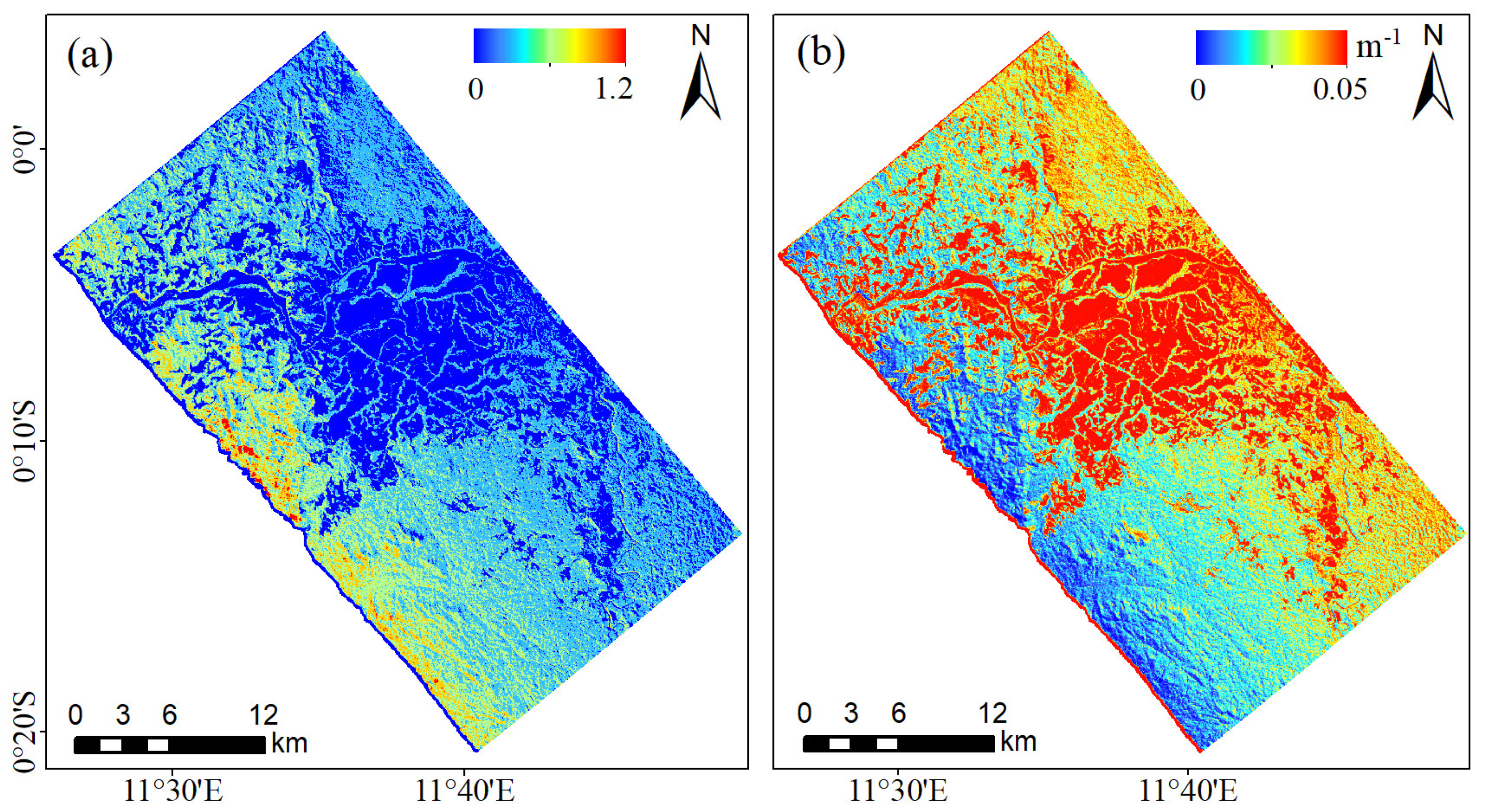
4.1. Volume Scattering Power

Following the generalized Stokes vector decomposition framework proposed by [28] and outlined in Section 2.2.1, the volume scattering power was extracted, as depicted in Figure 4a. This result indicates that the volume scattering power is mainly concentrated between 0 and 1.2. When compared to the forest height derived from LVIS LiDAR (Figure 3c), the derived volume scattering power exhibited a consistent spatial distribution, while taller canopy heights exhibited a higher power value. Notably, this study utilized the VH-VV polarization combination to extract the volume scattering power, since this dual-polarization combination is particularly suitable for calculating the volume scattering power in areas with taller vegetation [28]. Additionally, most current spaceborne SAR systems operate in this dual-polarization mode, such as the C-band Sentinel-1 mission, facilitating the subsequent application of the proposed method to large-scale forest height mapping.

4.2. Extinction Coefficient

Before extracting the extinction coefficients using the method described in Section 2.2.2, the forest canopy height data of ICESat-2 ATL08 were used to calculate the corresponding extinction coefficient using Equation (7). Subsequently, according to the geometric coordinates of the ICESat-2 sampling points, the input characteristic variables, including backscatter in the VV and VH channels, the incidence angle, and the terrain slope in the radar range direction, were extracted. Based on the aforementioned characteristic variables and training data (i.e., extinction coefficients on LiDAR samples), the random forest regression (RFR) machine learning algorithm was employed to construct the extinction coefficient prediction model. Additionally, to evaluate the prediction accuracy of the RFR model, the original datasets were divided into training data and test data in a 7:3 ratio. In this study, the RFR algorithm achieves an overall fine performance, with an ME of 1.09 × 10⁻⁴ m⁻¹ and an RMSE of 9.29 × 10⁻³ m⁻¹, which enables us to make accurate predictions for the extinction coefficients. Finally, the trained model was applied to predict the extinction coefficients for the entire study area, as shown in Figure 4b. It is worth noting that the extinction coefficients are presented in natural units of m⁻¹.

Figure 5 shows the importance distribution of each variable for the extinction coefficient prediction. The horizontal axis represents various variables, and the vertical axis represents the importance ratio. The result shows that VH backscatter is the most key variable for determining the extinction coefficient, followed by the local incidence angle (LocalInc), and the terrain slope along the radar range direction (Rngslope), while VV backscatter exhibits the least important.

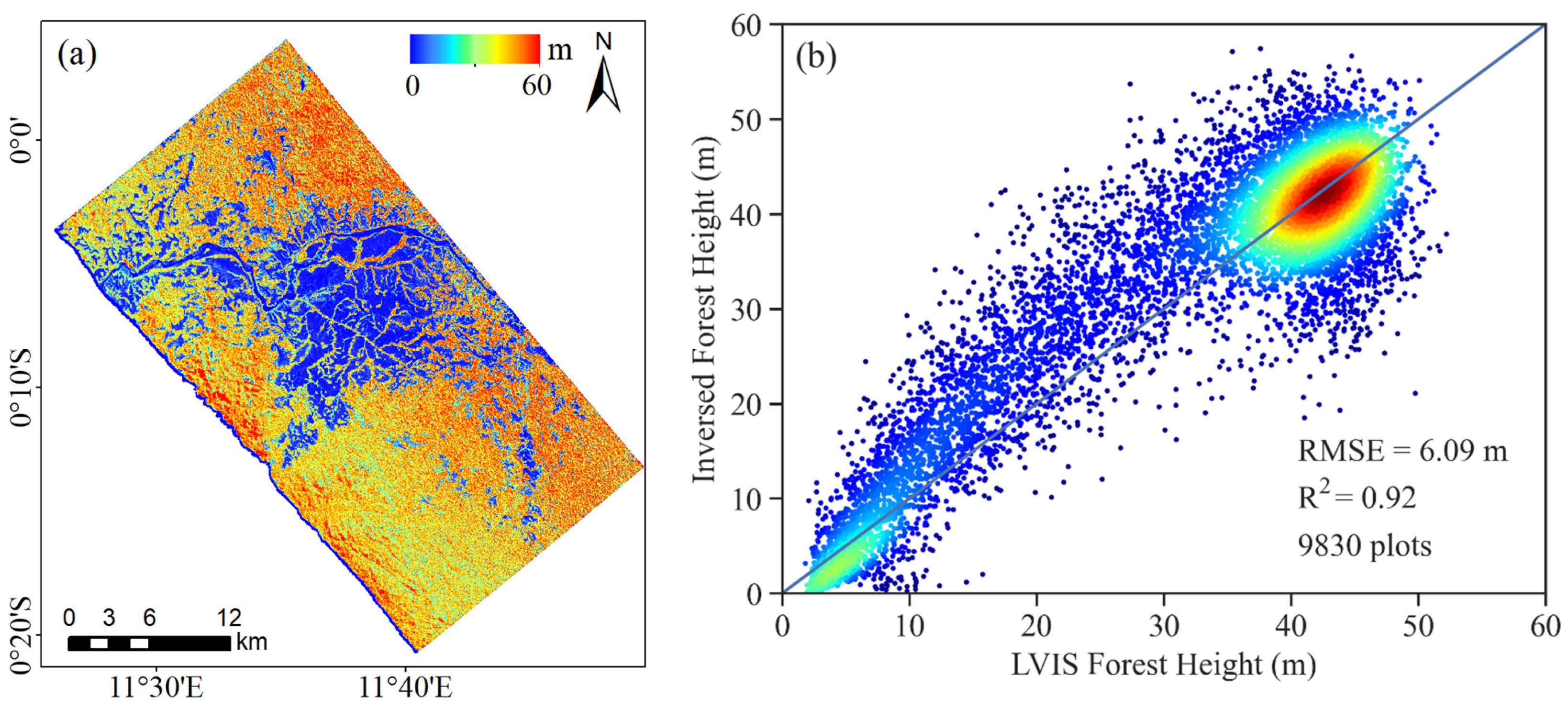
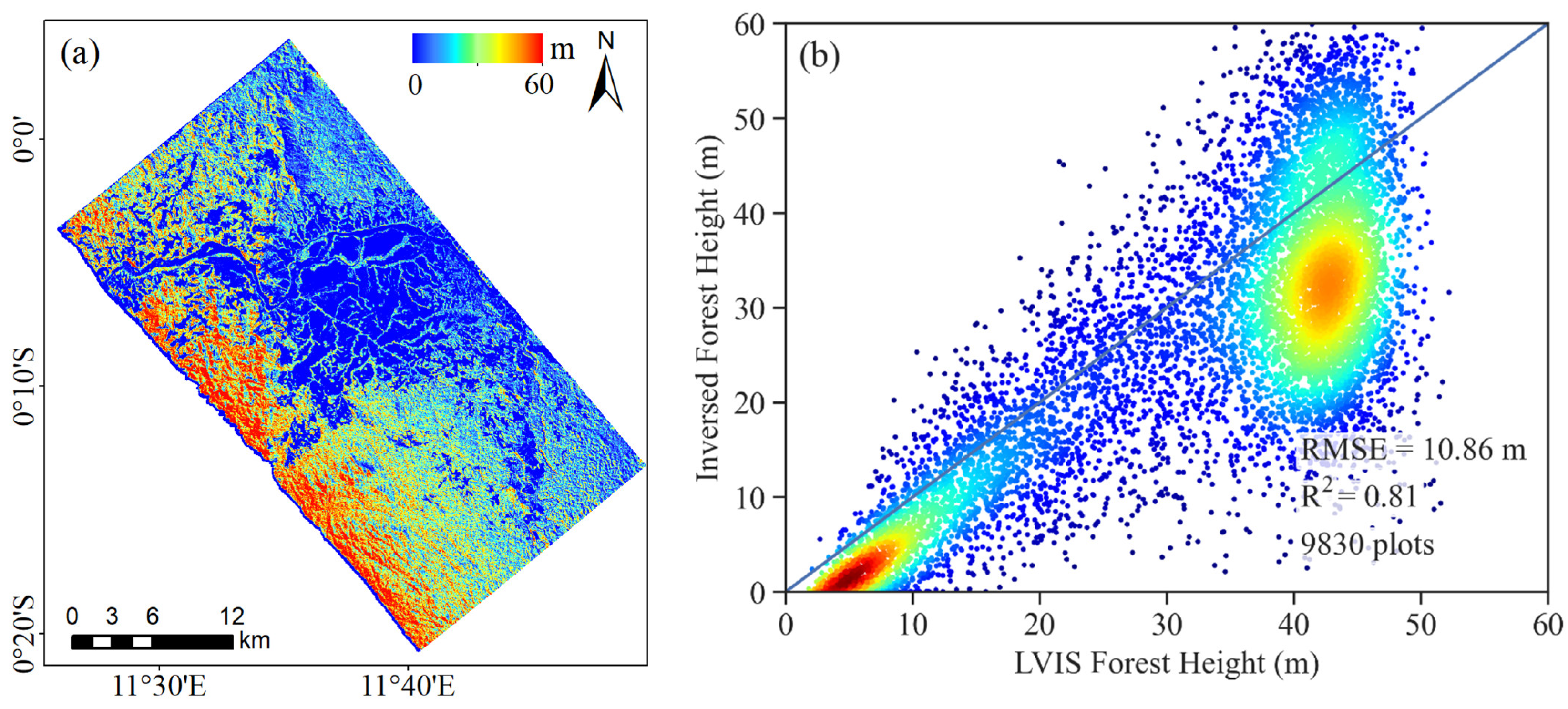
4.3. Forest Height Inversion

Using the calculated volume scattering power and the predicted extinction coefficient, we can calculate the forest canopy height using the semi-empirical inversion model presented in Equation (7). Figure 6a show the derived forest height map. By referring to the LVIS forest height map (Figure 3c), the proposed method is relatively more effective for tall forest stands, but it tends to overestimate the shorter stands. In areas with low vegetation, the L-band SAR has stronger penetration capabilities. As a result, the backscatter energy includes not only volume scattering but also a portion of dihedral scattering and ground scattering [42,43]; thereby, certain inversion errors could be introduced.

To further evaluate the derived forest height, a quantitative comparison was performed by regarding LVIS forest height data as the reference. To this aim, forest height is evaluated at the forest stand level, with the average forest height in a 10 × 10 window (192.00 m × 133.60 m). Additionally, the forest stands with a height less than 3 m were considered grassland and masked. We finally extracted a total of 9830 stands for the accuracy evaluation. The corresponding scatterplot is shown in Figure 6b. It is apparent that the forest height derived by the proposed method exhibits a reasonable agreement with the LVIS data, with a root mean square error (RMSE) of 6.09 m. In addition, a more detailed quantitative evaluation of the inversed forest height was conducted in a spatially continuous manner, supported by the LVIS forest height product. The evaluation of height errors across different forest heights is summarized in

Table 1. Statistical results of radar-based forest height (in meters) across different forest height classes.

	ME (m)	RMSE (m)
$\mathrm{shorter} \mathrm{forest} \mathrm{stands} \left(h_v\le 35 \mathrm{m}\right)$	3.70	6.72
$\mathrm{taller} \mathrm{forest} \mathrm{stands} \left(h_v>35 \mathrm{m}\right)$	−0.70	5.28

, using the mean error (ME) and the RMSE as statistical indicators to assess the height accuracy of the retrieved forest height. We observed an overestimation of canopy height in areas with shorter stands $\left(h_v\le 35 \mathrm{m}\right)$, as indicated by a positive ME of 3.70 m. On the contrary, the taller forest stands exhibited an overall lower bias of −0.70 m with respect to the LVIS forest height results.

5. Discussion

5.1. A Comparison between the Proposed Method and Existing Inversion Methods

By testing the proposed method in a classical tropical forest scenario, its effectiveness has been demonstrated. To further assess its suitability and advantages for forest height inversion, we conducted a comparative analysis between our approach and existing inversion methods.

Compared with the conventional PolInSAR inversion method based on the RVoG model, our approach demonstrated an improved performance, achieving an RMSE of 6.09 m, which is better than the RMSE of 8.68 m previously reported for the same Lope forest site in [32]. This may have two possible explanations. When the RVoG model is applied to single-baseline repeat-pass PolInSAR data, the uncertainty of temporal decorrelation can significantly reduce the accuracy of the forest estimation [25]. Although some previous studies proposed methods to compensate for temporal decorrelation, such as the RMoG model [13] and the RVoG-vtd model [44], this issue remains challenging to resolve. For instance, the study in [45] reported that the forest height inversion method using the RVoG-vtd model achieved an overall inversion accuracy of 7.72 m. In our approach, however, a single-temporal PolSAR image was used for the forest height inversion, which eliminated the effects of temporal decorrelation, leading to a potentially higher inversion accuracy. On the other hand, the performance of the conventional single-baseline PolInSAR inversion method based on the RVoG model depends on the sensitivity of the selected baseline [16,46]. Longer baselines produce larger vertical effective wave numbers and increased sensitivity to particularly low forests, and shorter baselines produce smaller vertical effective wave numbers, with reduced sensitivity to forest height. Therefore, to overcome the limitation of using a single baseline to invert forest height, various multi-baseline inversion algorithms have been proposed, such as the baseline selection method based on the vertical effective wave number [47], the method combining machine learning with LiDAR forest height [35,48] and the multi-baseline joint adjustment method [31,32]. For instance, Denbina et al. [35] approached the optimal baseline selection as a supervised classification problem and improved the inversion accuracy to 5.99 m by incorporating a small amount of sparse LiDAR forest height data. Cao et al. [31] proposed a multi-baseline forest height joint inversion method based on the complex least squares adjustment, achieving an overall inversion accuracy of 5.80 m. Although these methods exhibited significant improvements in the inversion accuracy, they do require a large volume of PolInSAR data or observation baselines to obtain satisfactory results. On the contrary, our results are comparable to theirs, but obtained with solely single-temporal PolSAR data.

In comparison to the forest height estimation method utilizing single-temporal PolSAR data [18], our approach demonstrates superior performance. To demonstrate this observation, we conducted a comparison analysis in which we utilized a similar idea proposed in [18], with the following steps: (1) an empirical model between the volume scattering power and LVIS RH100 metrics is established; (2) the forest height of the whole SAR scene is then derived from this fitted empirical model. In Figure 7a,b, the forest height results and validation plots are presented. It is apparent that this method tends to underestimate the height for all forest stands, achieving an RMSE of 10.86 m. This lower inversion accuracy can be attributed to the limitations of the use of such a linear model, as it is insufficient to describe the relationship between forest height and the characteristic parameters of PolSAR. Additionally, as stated in [18], this model should be utilized on larger homogeneous and higher biomass forest stands. When it comes to our approach, although we also utilized a semi-empirical inversion model (Equation (7)) to characterize the relationship between forest height and PolSAR parameters, we included an additional extinction coefficient that allows us to adaptively adjust the model to better suit specific forest stands and scenarios.

5.2. Limitations and Improvements for Further Work

To verify the applicability of the proposed method and explore avenues for further enhancements, it is crucial to thoroughly analyze the limiting factors.

Firstly, our results showed that forest height impacts the performance of the proposed method (see Table 1). In areas with taller vegetation, the proposed approach exhibited superior performance compared to areas with shorter forest stands. This may be due to the mismatch between the semi-empirical inversion model and the actual forest scenario. Ideally, the received radar signal in forested areas should be dominated by the volume scattering mechanism. However, in areas with shorter vegetation, the SAR signals can penetrate the forest layer, resulting in significant ground scattering contributions [49]. As a result, the assumption of negligible ground scattering energy in the derivation of Equation (7) becomes invalid. Therefore, one limitation that can be foreseen with our approach is its reduced effectiveness when applied to lower-forest conditions.

Secondly, in our approach, generating a wall-to-wall forest height product involves using machine learning to extract the extinction coefficient. This step is relatively time-consuming, which impacts the overall computational efficiency of the method. Therefore, it is crucial to consider the efficiency of the algorithms, especially when applied to large-scale inversion applications.

Based on these limitations, future research will focus on modeling that can simultaneously consider the contributions of various scattering mechanisms, such as volume scattering and ground scattering, to overcome the forest height inversion challenges in low-vegetation regions.

6. Conclusions

In this work, we introduced a new method for the estimation of forest height using a single-temporal dual-polarization PolSAR image, augmented by some sparse LiDAR data from the ICESat-2 mission. To validate the effectiveness of our proposed method, we conducted an experiment using the L-band UAVSAR data collected over Lope National Park. The experimental results demonstrated that our method successfully extracts forest height, and best correlated with the LVIS RH100 metric to an accuracy of 6.09 m. Compared with conventional PolInSAR forest height inversion methods, the proposed method exhibits superior performance and less dependency on interferometric data. Given the efficiency of the approach in this paper, it has the potential to enable wide-ranging mapping of forest height with spaceborne dual-polarization SAR missions, such as ESA’s Sentinel-1 and JAXA’s ALOS/PALSAR. However, for forest height mapping on a large scale, the enhancement in computational efficiency requires further research.

References

- Houghton, R.; Hall, F.; Goetz, S. Importance of Biomass in the Global Carbon Cycle. J. Geophys. Res.-Biogeosci. 2009, 114, G00E03. [Google Scholar] [CrossRef]
- Lei, Y.; Treuhaft, R.; Gonçalves, F. Automated Estimation of Forest Height and Underlying Topography over a Brazilian Tropical Forest with Single-Baseline Single-Polarization TanDEM-X SAR Interferometry. Remote Sens. Environ. 2021, 252, 112132. [Google Scholar] [CrossRef]
- Dubayah, R.; Blair, J.B.; Goetz, S.; Fatoyinbo, L.; Hansen, M.; Healey, S.; Hofton, M.; Hurtt, G.; Kellner, J.; Luthcke, S.; et al. The Global Ecosystem Dynamics Investigation: High-Resolution Laser Ranging of the Earth’s Forests and Topography. Sci. Remote Sens. 2020, 1, 100002. [Google Scholar] [CrossRef]
- Schneider, F.D.; Ferraz, A.; Hancock, S.; Duncanson, L.I.; Dubayah, R.O.; Pavlick, R.P.; Schimel, D.S. Towards Mapping the Diversity of Canopy Structure from Space with GEDI. Environ. Res. Lett. 2020, 15, 115006. [Google Scholar] [CrossRef]
- Sheng, Y.; Gong, P.; Biging, G.S. Model-Based Conifer-Crown Surface Reconstruction from High-Resolution Aerial Images. Photogramm. Eng. Remote Sens. 2001, 67, 957–965. [Google Scholar]
- Gong, P.; Mel, X.; Blglng, G.; Zhang, Z. Improvement of an Oak Canopy Model Extracted from Digital Photogrammetry. Photogramm. Eng. Remote Sens. 2002, 68, 919–924. [Google Scholar]
- Ni, W.; Ranson, K.J.; Zhang, Z.; Sun, G. Features of Point Clouds Synthesized from Multi-View ALOS/PRISM Data and Comparisons with LiDAR Data in Forested Areas. Remote Sens. Environ. 2014, 149, 47–57. [Google Scholar] [CrossRef]
- Zhu, J.; Fu, H.; Wang, C. Methods and Research Progress of Underlying Topography Estimation over Forest Areas by InSAR. Geomat. Inf. Sci. Wuhan Univ. 2018, 43, 2030–2038. [Google Scholar] [CrossRef]
- Zhu, J.; Fu, H.; Wang, C. Research Progress of “Penetration Mapping” of Earth Surface by PolInSAR. Acta Geod. Cartogr. Sin. 2022, 51, 983–995. [Google Scholar]
- Treuhaft, R.N.; Moghaddam, M.; van Zyl, J.J. Vegetation Characteristics and Underlying Topography from Interferometric Radar. Radio Sci. 1996, 31, 1449–1485. [Google Scholar] [CrossRef]
- Soja, M.J.; Persson, H.J.; Ulander, L.M.H. Estimation of Forest Biomass From Two-Level Model Inversion of Single-Pass InSAR Data. IEEE Trans. Geosci. Remote Sens. 2015, 53, 5083–5099. [Google Scholar] [CrossRef]
- Papathanassiou, K.P.; Cloude, S.R. Single-Baseline Polarimetric SAR Interferometry. IEEE Trans. Geosci. Remote Sens. 2001, 39, 2352–2363. [Google Scholar] [CrossRef]
- Lavalle, M.; Simard, M.; Hensley, S. A Temporal Decorrelation Model for Polarimetric Radar Interferometers. IEEE Trans. Geosci. Remote Sens. 2012, 50, 2880–2888. [Google Scholar] [CrossRef]
- Lavalle, M.; Hensley, S. Demonstration of Repeat-Pass POLINSAR Using UAVSAR: The RMOG Model. In Proceedings of the 2012 IEEE International Geoscience and Remote Sensing Symposium, Munich, Germany, 22–27 July 2012; pp. 5876–5879. [Google Scholar]
- Pourshamsi, M.; Garcia, M.; Lavalle, M.; Balzter, H. A Machine-Learning Approach to PolInSAR and LiDAR Data Fusion for Improved Tropical Forest Canopy Height Estimation Using NASA AfriSAR Campaign Data. IEEE J. Sel. Top. Appl. Earth Obs. Remote Sens. 2018, 11, 3453–3463. [Google Scholar] [CrossRef]
- Kugler, F.; Lee, S.-K.; Hajnsek, I.; Papathanassiou, K.P. Forest Height Estimation by Means of Pol-InSAR Data Inversion: The Role of the Vertical Wavenumber. IEEE Trans. Geosci. Remote Sens. 2015, 53, 5294–5311. [Google Scholar] [CrossRef]
- Chen, H.; Cloude, S.R.; Goodenough, D.G. Forest Canopy Height Estimation Using Tandem-X Coherence Data. IEEE J. Sel. Top. Appl. Earth Obs. Remote Sens. 2016, 9, 3177–3188. [Google Scholar] [CrossRef]
- Garestier, F.; Dubois-Fernandez, P.C.; Guyon, D.; Le Toan, T. Forest Biophysical Parameter Estimation Using L- and P-Band Polarimetric SAR Data. IEEE Trans. Geosci. Remote Sens. 2009, 47, 3379–3388. [Google Scholar] [CrossRef]
- García, M.; Saatchi, S.; Ustin, S.; Balzter, H. Modelling Forest Canopy Height by Integrating Airborne LiDAR Samples with Satellite Radar and Multispectral Imagery. Int. J. Appl. Earth Obs. Geoinf. 2018, 66, 159–173. [Google Scholar] [CrossRef]
- Pourshamsi, M.; Garcia, M.; Lavalle, M.; Pottier, E.; Balzter, H. Machine-Learning Fusion of Polsar and Lidar Data for Tropical Forest Canopy Height Estimation. In Proceedings of the IGARSS 2018—2018 IEEE International Geoscience and Remote Sensing Symposium, Valencia, Spain, 22–27 July 2018; pp. 8108–8111. [Google Scholar]
- Pourshamsi, M.; Xia, J.; Yokoya, N.; Garcia, M.; Lavalle, M.; Pottier, E.; Balzter, H. Tropical Forest Canopy Height Estimation from Combined Polarimetric SAR and LiDAR Using Machine-Learning. ISPRS J. Photogramm. Remote Sens. 2021, 172, 79–94. [Google Scholar] [CrossRef]
- Cloude, S. Polarisation: Applications in Remote Sensing, 1st ed.; Oxford University Press: Oxford, UK; New York, NY, USA, 2010; ISBN 978-0-19-956973-1. [Google Scholar]
- Neuenschwander, A.; Pitts, K. The ATL08 Land and Vegetation Product for the ICESat-2 Mission. Remote Sens. Environ. 2019, 221, 247–259. [Google Scholar] [CrossRef]
- Treuhaft, R.N.; Siqueira, P.R. Vertical Structure of Vegetated Land Surfaces from Interferometric and Polarimetric Radar. Radio Sci. 2000, 35, 141–177. [Google Scholar] [CrossRef]
- Lee, S.-K.; Kugler, F.; Papathanassiou, K.P.; Hajnsek, I. Quantification of Temporal Decorrelation Effects at L-Band for Polarimetric SAR Interferometry Applications. IEEE J. Sel. Top. Appl. Earth Obs. Remote Sens. 2013, 6, 1351–1367. [Google Scholar] [CrossRef]
- Cloude, S.R.; Papathanassiou, K.P. Three-Stage Inversion Process for Polarimetric SAR Interferometry. IEE Proc.-Radar Sonar Navig. 2003, 150, 125–134. [Google Scholar] [CrossRef]
- Freeman, A. Fitting a Two-Component Scattering Model to Polarimetric SAR Data From Forests. IEEE Trans. Geosci. Remote Sens. 2007, 45, 2583–2592. [Google Scholar] [CrossRef]
- Mascolo, L.; Cloude, S.R.; Lopez-Sanchez, J.M. Model-Based Decomposition of Dual-Pol SAR Data: Application to Sentinel-1. IEEE Trans. Geosci. Remote Sens. 2022, 60, 1–19. [Google Scholar] [CrossRef]
- Sugimoto, R.; Nakamura, R.; Tsutsumi, C.; Yamaguchi, Y. Extension of Scattering Power Decomposition to Dual-Polarization Data for Tropical Forest Monitoring. Remote Sens. 2023, 15, 839. [Google Scholar] [CrossRef]
- Sharma, J.J.; Hajnsek, I.; Papathanassiou, K.P.; Moreira, A. Estimation of Glacier Ice Extinction Using Long-Wavelength Airborne Pol-InSAR. IEEE Trans. Geosci. Remote Sens. 2013, 51, 3715–3732. [Google Scholar] [CrossRef]
- Cao, S.; Fu, H.; Zhu, J.; Xie, Y.; Song, T. A Forest Height Joint Inversion Method Using Multibaseline PolInSAR Data. IEEE Geosci. Remote Sens. Lett. 2022, 19, 2508105. [Google Scholar] [CrossRef]
- Luo, H.; Yue, C.; Yuan, H.; Wang, N.; Chen, S. A Method for Forest Canopy Height Inversion Based on UAVSAR and Fourier–Legendre Polynomial—Performance in Different Forest Types. Drones 2023, 7, 152. [Google Scholar] [CrossRef]
- Marshak, C.; Simard, M.; Duncanson, L.; Silva, C.A.; Denbina, M.; Liao, T.-H.; Fatoyinbo, L.; Moussavou, G.; Armston, J. Regional Tropical Aboveground Biomass Mapping with L-Band Repeat-Pass Interferometric Radar, Sparse Lidar, and Multiscale Superpixels. Remote Sens. 2020, 12, 2048. [Google Scholar] [CrossRef]
- Guliaev, R.; Cazcarra-Bes, V.; Pardini, M.; Papathanassiou, K. Forest Height Estimation by Means of TanDEM-X InSAR and Waveform Lidar Data. IEEE J. Sel. Top. Appl. Earth Obs. Remote Sens. 2021, 14, 3084–3094. [Google Scholar] [CrossRef]
- Denbina, M.; Simard, M.; Hawkins, B. Forest Height Estimation Using Multibaseline PolInSAR and Sparse Lidar Data Fusion. IEEE J. Sel. Top. Appl. Earth Obs. Remote Sens. 2018, 11, 3415–3433. [Google Scholar] [CrossRef]
- El Moussawi, I.; Ho Tong Minh, D.; Baghdadi, N.; Abdallah, C.; Jomaah, J.; Strauss, O.; Lavalle, M. L-Band UAVSAR Tomographic Imaging in Dense Forests: Gabon Forests. Remote Sens. 2019, 11, 475. [Google Scholar] [CrossRef]
- Labriere, N.; Tao, S.; Chave, J.; Scipal, K.; Toan, T.L.; Abernethy, K.; Alonso, A.; Barbier, N.; Bissiengou, P.; Casal, T.; et al. In Situ Reference Datasets From the TropiSAR and AfriSAR Campaigns in Support of Upcoming Spaceborne Biomass Missions. IEEE J. Sel. Top. Appl. Earth Obs. Remote Sens. 2018, 11, 3617–3627. [Google Scholar] [CrossRef]
- Lavalle, M.; Hawkins, B.; Hensley, S. Tomographic Imaging with UAVSAR: Current Status and New Results from the 2016 AfriSAR Campaign. In Proceedings of the 2017 IEEE International Geoscience and Remote Sensing Symposium (IGARSS), Fort Worth, TX, USA, 23–28 July 2017; pp. 2485–2488. [Google Scholar] [CrossRef]
- Fatoyinbo, T.; Armston, J.; Simard, M.; Saatchi, S.; Denbina, M.; Lavalle, M.; Hofton, M.; Tang, H.; Marselis, S.; Pinto, N.; et al. The NASA AfriSAR Campaign: Airborne SAR and Lidar Measurements of Tropical Forest Structure and Biomass in Support of Current and Future Space Missions. Remote Sens. Environ. 2021, 264, 112533. [Google Scholar] [CrossRef]
- Blair, J.B.; Rabine, D.L.; Hofton, M.A. The Laser Vegetation Imaging Sensor: A Medium-Altitude, Digitisation-Only, Airborne Laser Altimeter for Mapping Vegetation and Topography. ISPRS J. Photogramm. Remote Sens. 1999, 54, 115–122. [Google Scholar] [CrossRef]
- Hofton, M.A.; Rocchio, L.E.; Blair, J.B.; Dubayah, R. Validation of Vegetation Canopy Lidar Sub-Canopy Topography Measurements for a Dense Tropical Forest. J. Geodyn. 2002, 34, 491–502. [Google Scholar] [CrossRef]
- Wu, F.; Wang, C.; Zhang, H.; Zhang, B.; Tang, Y. Rice Crop Monitoring in South China with RADARSAT-2 Quad-Polarization SAR Data. IEEE Geosci. Remote Sens. Lett. 2011, 8, 196–200. [Google Scholar] [CrossRef]
- Xie, Q.; Zhu, J.; Lopez-Sanchez, J.M.; Wang, C.; Fu, H. A Modified General Polarimetric Model-Based Decomposition Method with the Simplified Neumann Volume Scattering Model. IEEE Geosci. Remote Sens. Lett. 2018, 15, 1229–1233. [Google Scholar] [CrossRef]
- Simard, M.; Denbina, M. An Assessment of Temporal Decorrelation Compensation Methods for Forest Canopy Height Estimation Using Airborne L-Band Same-Day Repeat-Pass Polarimetric SAR Interferometry. IEEE J. Sel. Top. Appl. Earth Obs. Remote Sens. 2018, 11, 95–111. [Google Scholar] [CrossRef]
- Xing, C.; Zhang, T.; Wang, H.; Zeng, L.; Yin, J.; Yang, J. A Novel Four-Stage Method for Vegetation Height Estimation with Repeat-Pass PolInSAR Data via Temporal Decorrelation Adaptive Estimation and Distance Transformation. Remote Sens. 2021, 13, 213. [Google Scholar] [CrossRef]
- Liao, Z.; He, B.; van Dijk, A.I.J.M.; Bai, X.; Quan, X. The Impacts of Spatial Baseline on Forest Canopy Height Model and Digital Terrain Model Retrieval Using P-Band PolInSAR Data. Remote Sens. Environ. 2018, 210, 403–421. [Google Scholar] [CrossRef]
- Lee, S.-K.; Fatoyinbo, T.E.; Lagomasino, D.; Feliciano, E.; Trettin, C. Multibaseline TanDEM-X Mangrove Height Estimation: The Selection of the Vertical Wavenumber. IEEE J. Sel. Top. Appl. Earth Obs. Remote Sens. 2018, 11, 3434–3442. [Google Scholar] [CrossRef]
- Xie, Y.; Fu, H.; Zhu, J.; Wang, C.; Xie, Q. A LiDAR-Aided Multibaseline PolInSAR Method for Forest Height Estimation: With Emphasis on Dual-Baseline Selection. IEEE Geosci. Remote Sens. Lett. 2020, 17, 1807–1811. [Google Scholar] [CrossRef]
- Jagdhuber, T.; Hajnsek, I.; Bronstert, A.; Papathanassiou, K.P. Soil Moisture Estimation Under Low Vegetation Cover Using a Multi-Angular Polarimetric Decomposition. IEEE Trans. Geosci. Remote Sens. 2013, 51, 2201–2215. [Google Scholar] [CrossRef]