Article

Hydrologic Perturbation Is a Key Driver of Tree Mortality in Bottomland Hardwood Wetland Forests of North Carolina, USA

by
Maricar Aguilos
1,*,
Cameron Carter
1,
Brandon Middlebrough
1,
James Bulluck
1,
Jackson Webb
1,
Katie Brannum
1,
John Oliver Watts
1,
Margaux Lobeira
1,
Ge Sun
2,
Steve McNulty
2 and
John King
1
1
Department of Forestry and Environmental Resources, North Carolina State University, Raleigh, NC 27695, USA
2
Eastern Forest Environmental Threat Assessment Center, Southern Research Station, USDA Forest Service, Research Triangle Park, NC 27709, USA
*
Author to whom correspondence should be addressed.
Forests 2025, 16(1), 39; https://doi.org/10.3390/f16010039
Submission received: 28 November 2024 / Revised: 24 December 2024 / Accepted: 26 December 2024 / Published: 29 December 2024
(This article belongs to the Section Forest Ecology and Management)

Abstract

:
Bottomland hardwood wetland forests along the Atlantic Coast of the United States have been changing over time; this change has been exceptionally apparent in the last two decades. Tree mortality is one of the most visually striking changes occurring in these coastal forests today. Using 2009–2019 tree mortality data from a bottomland hardwood forest monitored for long-term flux studies in North Carolina, we evaluated species composition and tree mortality trends and partitioned variance among hydrologic (e.g., sea level rise (SLR), groundwater table depth), biological (leaf area index (LAI)), and climatic (solar radiation and air temperature) variables affecting tree mortality. Results showed that the tree mortality rate rose from 1.64% in 2009 to 45.82% over 10 years. Tree mortality was primarily explained by a structural equation model (SEM) with R2 estimates indicating the importance of hydrologic (R2 = 0.65), biological (R2 = 0.37), and climatic (R2 = 0.10) variables. Prolonged inundation, SLR, and other stressors drove the early stages of ‘ghost forest’ formation in a formerly healthy forested wetland relatively far inland from the nearest coastline. This study contributes to a growing understanding of widespread coastal ecosystem transition as the continental margin adjusts to rising sea levels, which needs to be accounted for in ecosystem modeling frameworks.

1. Introduction

Forested wetlands offer various physical, chemical, and biological ecosystem functions [1,2]. However, because of their topographic location, forested wetlands are exposed to multiple threats of climate change [3]. Global projection showed that from 20 to 90 percent of the current forested wetland areas will be lost due to sea level rise [4,5,6]. A report showed that 3.4 million km2 has been lost since 1700 due to wetland drainage, urbanization, wetland cultivation, and other land conversions [7]. Climate change is rapidly transforming coastal ecosystems, which have been disproportionately large yet highly vulnerable [8,9]. Widespread coastal wetland forests decline due to climate change and other natural and anthropogenic disturbances have been reported, e.g., Africa has lost 2.1% of its mangrove ecosystem from 1996 to 2020 [10]; Indonesia lost 800,000 ha of coastal wetland over the past 30 years [11,12]; India faced a 47% loss in the coastal wetland carbon storage due to an increase in surface water salinity by 47.6% from 2017 to 2021 [13]; Brazil lost 21,000 ha mangrove forest per year over the last decade [14,15]; and there is a 97% accuracy in predicting estuarine forest loss in Amazon floodplains due to anthropogenic and climatic impacts [16].
Large-scale tree mortality is prevalent in bottomland woody-plant-dominated coastal ecosystems [17]. Widespread mortality within these forests, referred to as ‘ghost forests’, is becoming globally evident [18,19]. However, the mechanisms of coastal ecosystem transition to interacting hydrologic, biotic, and climatic perturbations remain poorly understood [20].
The coastal wetlands of North Carolina also faced the impact of climate change and anthropogenic pressures [9,21,22]. Other observations found that sea level rise (SLR) slowly degraded existing wetlands, increasing the tree mortality of inland wetland forests [23]. Any changes in key environmental and biological factors that alter individual species’ physiological functioning or survival can profoundly affect ecosystem structure and function [3]. Therefore, understanding the ecological resilience of forest tree species to the changing environment is important.
Predictive modeling frameworks have already been established for coastal tree mortality [24,25,26,27]. Such modeling frameworks are critical to predicting future ghost forest formation. A structural equation model (SEM) could enable representation of the compounding effects of biologic, hydrologic, and climatic drivers leading to tree mortality and could be used as a reference for future investigations to elucidate the formation of ghost forests amidst a changing climate.
Widespread tree mortality in coastal ecosystems of the Southeast US occurs within a backdrop of the combined effects of SLR, prolonged inundation, and declining LAI [28,29,30], commonly with nonlinear interactions that challenge modeling efforts. A single mechanism does not govern mortality rates but rather a combination of various controlling aspects affecting the survival of trees. These knowledge gaps pose huge modeling uncertainties regarding the timing and intensity of ghost forest formation and their subsequent consequences on various ecosystem functions [31]. It is imperative to understand the drivers and processes of wetland forest tree mortality in relation to a changing climate, coupled with biological and hydrologic drivers, in order to predict forest loss. Driven by the growing concern for more wetland studies to evaluate the key drivers of widespread tree mortality, we bridge this research gap and focus our attention on the factors governing unabated forest loss to answer the following questions: (1) why has the long-term trend in tree mortality never recovered? (2) how do hydrologic, biologic, and climatic drivers interact to cause this widespread mortality? (3) Which species are primarily affected by these climate-change-related drivers of change? Thus, in this study, we draw attention to the role of interacting drivers of tree mortality, presenting a long-term (2009–2019) record of observations on tree mortality, highlighting the rapid pace of change yet are scarce for coastal wetland forests.
Here, we (1) examine the trends in tree mortality in association with key drivers, such as changes in hydrology (e.g., SLR, GWT, etc.), leaf area index, and other climatic variables associated with climate change; (2) utilize an SEM framework to evaluate the effects of biological, hydrologic, and climatic drivers on forest tree mortality; (3) characterize species vulnerability to the drivers of change over the long-term, which is largely missing to date. Based on empirical observations, we hypothesized that tree mortality is primarily driven by prolonged inundation. Our approach is one of the first studies that integrates multi-faceted and interlacing factors driving tree mortality to understand these complex interactions. This work contributes to understanding forest mortality and ecosystem dynamics in disturbed wetland forests and, in doing so, develops a modeling framework that advances the predictive capacity of ghost forest formation based on broad-scale environmental controls of tree mortality and ecosystem processes.

2. Materials and Methods
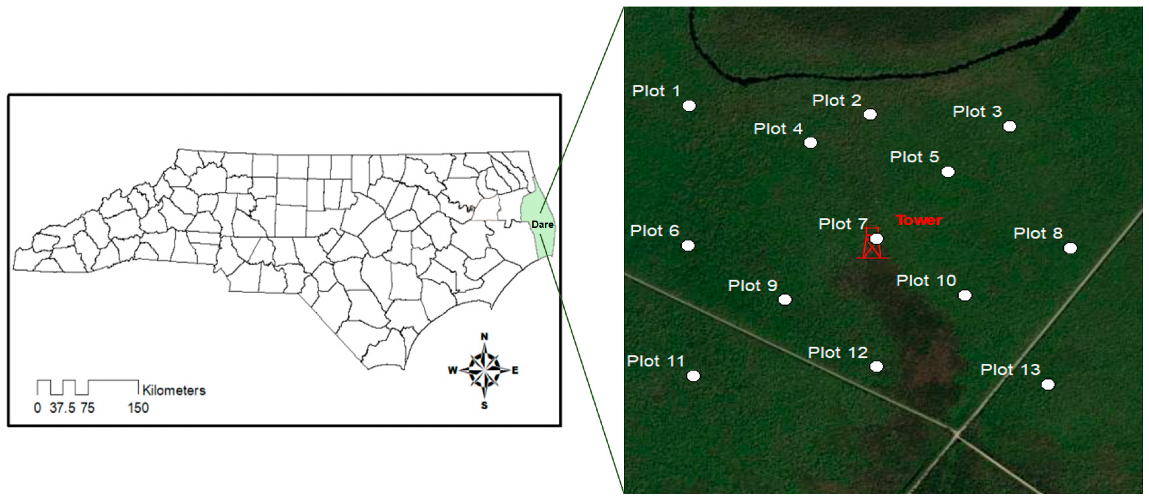
2.1. The Study Site

This study was conducted at the Alligator River National Wildlife Refuge (ARNWR) in Dare County, North Carolina, USA (35°45′16.44″ N and 75°54′13.64″) (Figure 1). The refuge is the second largest protected area in North Carolina, with a total area of 99,347 hectares. However, 1151 hectares were lost to the sea in recent decades, and an estimated 19,300 hectares of forested habitat is rapidly transitioning to marshland [32]. Currently, the site is experiencing chronic inundation due in part to the impediment of groundwater that drains into the sea, which is caused by rising sea levels. As reported in other studies, when the sea level rises, the lower wetland boundary recedes, causing inundation of coastal wetlands [4,5,6]. The rising sea level interferes with the establishment and survival of vegetation in our site, as observed in other studies, altering the species’ dominance zonation along the changing seaward–landward gradient [8,21,33,34].
Vegetation at the site is characterized as a natural coastal bottomland hardwood forest (i.e., forested wetland). Common species include American holly (Ilex opaca), tupelo (Nyssa spp.), sweetgum (Liquidambar styraciflua), loblolly pine (Pinus taeda), red maple (Acer rubrum), and other wetland species. The average canopy height of trees is 23 m, with an estimated tree density of 2320 trees ha−1. The soil is a Pungo series Haplosaprist with a 0.3–1.0 m thick organic layer. The site has an elevation of <1 m above sea level. The average annual rainfall was 1168 ± 204 mm (1981–2019), and the average temperature was 15.8 ± 1.8 °C (2005–2019). More descriptions of the study site can be found in previous reports [30,35,36].

2.2. Mortality Rate Calculation

In 2009, a total of 13 circular 7 m radius vegetation plots were established for vegetative surveys (Figure 1). All tree species within each plot with a diameter-at-breast height (DBH, i.e., 1.4 m above the floor) more than 2.5 cm were identified, marked, and measured. Measurements were made every winter season between December and March, from 2009 to 2019. Inside the measurement plot, downed trees or standing dead trees were identified and counted as mortality. We followed the commonly used mortality rate measure from various studies [37,38]. The mortality rate measure, λ, is calculated as follows:
λ = ln n 0 ln ( n t ) t
where λ is the mortality rate, n is the total number of trees of all species, n0 is the number of trees during the previous census date, nt are the number of surviving trees to time t (annually). The time between the two tree censuses is t.

2.3. The Key Drivers of Tree Mortality

2.3.1. Hydrologic Variables

We used the latent heat flux (LE, W m−2) derived from the flux tower to compute evapotranspiration (ET). Daily ET (representing the canopy evaporation, transpiration, and soil evaporation) was taken from the eddy covariance flux tower established within the experimental site. Daily ET was the sum of 30 min ET and compiled as the monthly sum for analysis. ET was converted from latent heat (LE) [36,39].
E T = L E λ
where λ (J kg−1) = 103 × (2500 − 2.37 × Ta) and Ta = Air temperature in °C (Celsius).
Potential evapotranspiration (PET) was estimated using the Priestley–Taylor method [40,41]. The Priestley–Taylor equation [42] is given as follows:
P E T = α   Δ   R n G λ ν   ( Δ + γ )
In this equation, PET is the potential evapotranspiration in mm d−1, and α is an empirical constant accounting for the vapor pressure deficit and resistance values. λν is the volumetric latent heat of vaporization, 2453 MJ m−3. Δ is the slope of the saturation vapor pressure–temperature curve (kPa per °C). γ is the psychrometric constant (kPa per °C). Rn is the net radiation in MJ m−2 d−1, and G is the soil heat flux density in MJ m−2 d−1.
We used a rain gauge (TE-525, Campbell Scientific Inc., Logan, UT, USA) to measure precipitation. The groundwater table depth (WTD) was determined using an ultrasonic water level datalogger (Infinities, Port Orange, FL, USA), with data in 2017 removed due to instrument errors. The water table instrument was mounted on the ground inside a perforated pipe with a continuous automated data collection system all year round. The data was averaged in a 30 min data resolution, and data retrieval was performed daily using a modem for remote data downloading. The measurement started in January 2009 and continued until 2019. We obtained our sea level data from NOAA tide gauges in Oregon Inlet Marina, North Carolina (https://tidesandcurrents.noaa.gov/sltrends/ accessed on 20 August 2024).

2.3.2. Biological Variables

The leaf area index (LAI) from 2000 to 2019 was obtained from the Global Land Surface Satellite (GLASS) LAI datasets [43] with the Moderate Resolution Imaging Spectroradiometer (MODIS) surface reflectance data at an 8-day and 1 km resolution.

2.3.3. Climatic Variables

We used a temperature probe (HMP45AC, Vaisala, Finland) to measure air temperature. We also used a radiation sensor (CNR-1, Kipp & Zonen, Delft, The Netherlands) to measure net radiation (CNR-1, Kipp & Zonen, Delft, The Netherlands). These climate variables were obtained from the US-NC4 flux tower data.

2.4. Modeling the Effects of Key Drivers on Tree Mortality

One type of probabilistic model that permits the specification of multiple causal pathways is SEMs (structural equation models) [44]. A chi-square test is used to assess the validity of the proposed SEM, and the p-value needs to be greater than 0.05 (Shipley, 2016). Measured variables were log-transformed in order to prevent data normality-related errors. The Shapiro–Wilk Univariate normality test and Mardia Multivariate normality test were applied to assess normality and skewness using the MVN package. We built our SEM based on our assumption that the effects of biological (represented by LAI), hydrological (P, PET, ET, GWT, and SLR), and climatic (Rn and Tair) variables impact tree mortality. The SEM was built using the sem() function lavaan package in R [44].

2.5. Other Statistical Analysis and Visualization

Statistically significant trends were determined using the nonparametric Mann–Kendall (MK) method [45,46,47]. When a positive value of standardized test statistic Z was found, it indicates an increasing trend in the rainfall time series, whereas negative Z values indicate a negative trend. If |Z| > Z1 − ∝/2, (H0) is rejected, and a statistically significant trend exists in the time series. The critical value of Z1 − ∝/2 for a p value of 0.05 from the standard normal table is 1.96.
Histogram and bar plots were generated using the ggplot2, ggpubr, plotly, tidyverse, and reshape packages in R. All analyses were performed using R version 4.2.3. [48].

3. Results

3.1. Species Composition and Tree Density

Among all the seven major species found at the study site (Figure 2; Table 1), American holly (I. opaca) had the lowest number of trees (10 trees ha−1), constituting only 3% of the entire tree population (Figure 2d). Species of the genus Nyssa had the highest tree density (140 trees ha−1), accounting for 38% of the total population (Figure 2h).

3.2. Inter-Annual Mortality Rates

The tree mortality rate rose from 1.64% in 2009 to 45.82% after 10 years (Table 1). The total number of downed trees accounted for most of the cumulative annual mortality (R2 = 0.99, p < 0.05), compared to the cumulative standing dead trees (R2 = 0.95, p < 0.05, Table 1).

3.3. Mortality Rate per Species

At the end of the measurement period in 2019, Persea palustris had the highest mortality rate (67.58%) of the angiosperms, while Ilex opaca had the lowest (10.54%). The species with the highest tree density (140 TPH) was Nyssa spp., yet the mortality rate of this species was 43.08% in 2019 (Table 1). The 69% mortality rate of Pinus taeda at the end of the measurement period was the highest of any species.

3.4. Variations of Predictor Variables

3.4.1. LAI—The Biological Driver

The satellite leaf area index (LAI) estimates varied from 2.77 to 3.43 (mean = 3.09 ± 0.18) during the monitoring period. We were able to detect a declining trend in LAI from 2009 to 2019 (p < 0.05) that coincided with increasing cumulative mortality.

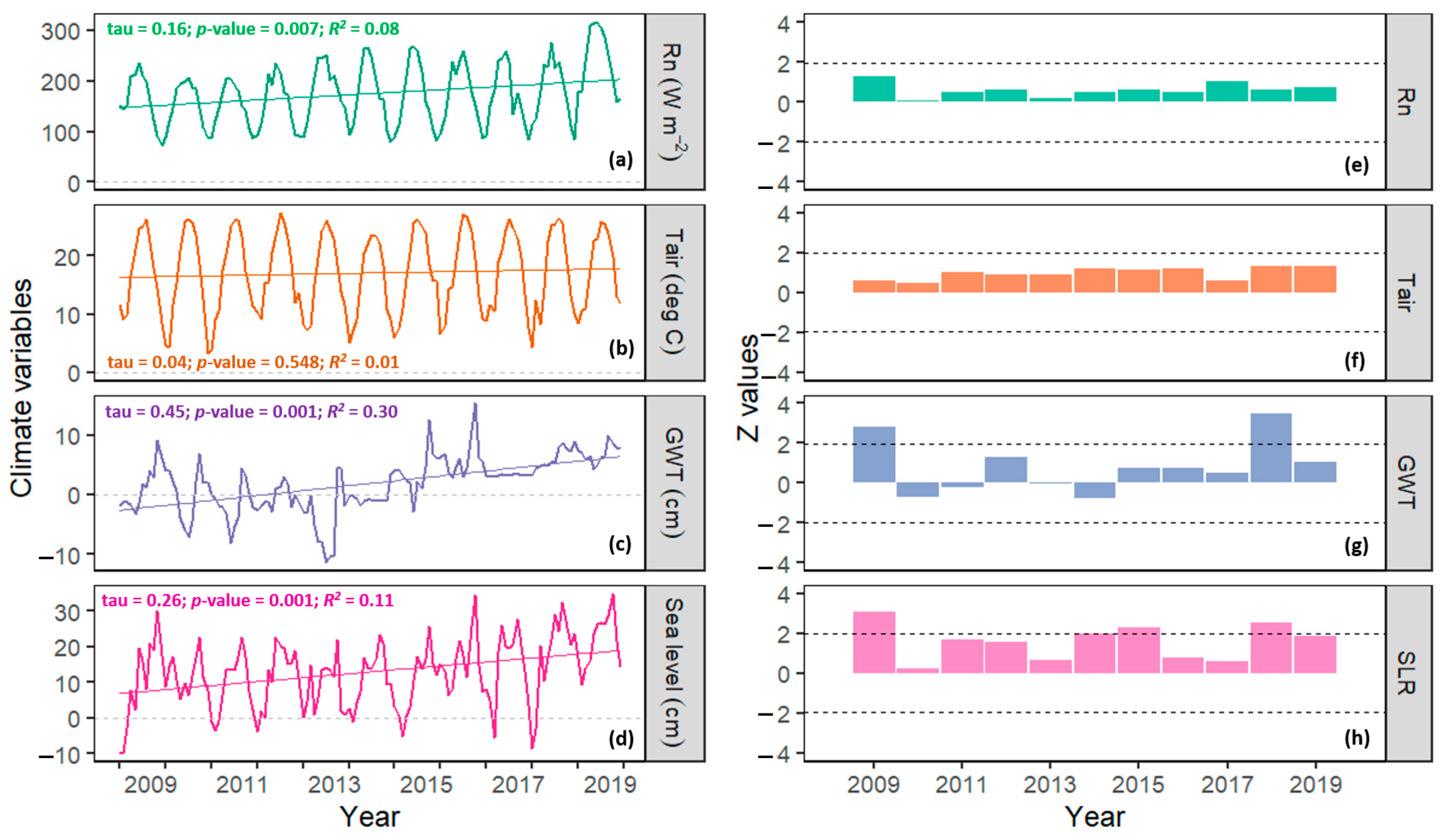
3.4.2. Hydrologic Drivers

The monthly SLR was erratic, although a gradually increasing trend can be observed cumulatively (R2 = 0.11; p < 0.05; Figure 3d,h). From 2009 to 2019, the average sea level was 12.9 cm (relative to a pre-determined reference measurement level), varying from 8.6 cm to 21.5 cm. The increasing trend in sea level coincides with an increasing relative groundwater table depth (GWT). The GWT rose from −4.3 cm (below the ground surface) to 1.2 cm (above ground) from 2009 to 2014, relative to a reference point [5], and from 3.2 cm to 6.9 cm above the land surface from 2015 onwards (R2 = 0.30; p < 0.05; Figure 3c,g). The flux tower is ~20 km away from the Croatan Sound and ~40 km from the Atlantic Ocean. Therefore, any increase in sea level only slightly increases GWT at our site, yet it is still detectable.
The annual average precipitation (P) was 1280 mm (minimum = 919 mm, maximum = 1511 mm). The annual average amount of evapotranspiration (ET) never exceeded P, except in 2019. ET was only 42%–71% of P from 2009 to 2018. The average ET over the years was 765 mm, ranging from 500 mm to 982 mm. On the other hand, PET had an average of 950 mm and varied from 950 mm to 1116 mm. It is expected that a reduction in water loss by ET will occur when mortality is reduced, which denotes a reduction in LAI. However, our results showed no significant correlation of LAI with ET (R2 < 0.01, p > 0.05).

3.4.3. Climatic Drivers

From 2009 to 2019, the average monthly net radiation (Rn) was 175.3 W m−2, ranging from 150.2 W m−2 to 242.0 W m−2. A sudden increase in Rn of 66.68 W m−2 higher than the monitoring period average occurred in 2019, although it was not significantly different from other years (p > 0.05; Figure 3a). The average air temperature varied from 15.5 °C to 17.8 °C with no statistically significant inter-annual differences (p > 0.05; Figure 3b).

3.5. Drivers of Tree Mortality

Tree mortality was explained by SEM with R2 estimates mainly by composite hydrologic variables (R2 = 0.65), biological (R2 = 0.37), and climatic (R2 = 0.10) (Figure 4). From 2005 to 2019, and across all plots, hydrologic variables (SLR, R2 = 0.83 and GWT, R2 = 0.81) primarily drove tree mortality from the hydrologic latent component with a highly significant positive effect on tree mortality (Figure 4).
In high water level situations, forested wetland tree cover decreases (and thus low LAI), thereby reducing water consumption through transpiration. This may decrease evapotranspiration losses at the ecosystem scale. Yet, ET only made a slight contribution (R2 = 0.15) from the composite hydrologic variables affecting tree mortality (Figure 4).
Biological variables, represented by LAI, explained 48% of the variation in the biological component and had a negative significant effect, with higher mortality and decreased LAI. The relatively low variance explained by LAI on tree mortality suggests that other plant-based factors may have more impact than LAI. Meanwhile, Rn (R2 = 0.42) in the climatic latent variable affected tree mortality more than air temperature (Figure 4).

4. Discussion

4.1. Species Adaptation to Inundation

Flood tolerance is often a determining factor in species composition and abundance in low-lying, wet sites. Flood-tolerant species may develop anatomical adaptations, including forming parenchyma tissues, developing hypertrophied lenticels, and producing adventitious water roots that facilitate oxygen uptake by the roots [49,50].
Our study showed that Nyssa spp. and Persea palustris are well adapted to high levels of inundation. Studies assessing wetland species composition classify black gum (Nyssa sylvatica) as the most flood-tolerant species in bottomland and floodplain forests [51,52,53]. This is consistent with our vegetative surveys, where tupelos had the highest tree density, more than double the average tree density of all other species, at 140 trees ha−1. Loblolly pine, red maple, and sweetgum may tolerate inundation for a short period of time [54]. Loblolly pine is considered moderately flood-tolerant; it typically can only withstand short periods of flooded conditions [54]. Moreover, in a flood zone area, a study indicated the flood tolerance characteristics of red maple [50]. Red maple has a high genetic variability and flood tolerance [55]. It can grow on a wider range of soil characteristics and elevation than other species [50].

4.2. Tree Mortality

Widespread mortality in ghost forests is the most devastating indicator of wetlands affected by SLR, saltwater intrusion, and other extreme events [18,32]. In our study, the rapidly increasing trend in tree mortality, from only six trees ha−1 in 2009 to 136 trees ha−1 in 2019, was surprising and concerning, as it appears our site is on a trajectory to soon become a ‘ghost forest’.
We found that bald cypress, sweetgum, and American holly were among the species with low mortality rates. Among these species, bald cypress is considered superior in terms of flooding resilience. The bald cypress is a large deciduous conifer tree native to the US Southeast, commonly dominating the coastal freshwater wetlands [56]. Although we did not monitor species adaptation in our study, some authors reported that bald cypress seedlings can withstand flooding for up to 45 days, but long-term submergence of the foliage results in high mortality rates [53]. Bald cypress is known to persist for years after the wetland site where it grows has been impacted by saltwater intrusion [57]. These characteristics may explain why bald cypress had a lower mortality rate at our site. Further study is needed to understand the physiological mechanisms behind the adaptive capacity of bald cypress.
Loblolly pine experienced the highest mortality. We attribute the leading cause of mortality to chronic hydrologic stress in conjunction with wood-boring insects, such as the southern pine beetle (Dendroctinous frontalis), the black turpentine beetle (Dendroctinous terebrans), or Ips engraver beetles (Ips calligraphus, Ips grandicollis, and Ips avulsus) (Figure 5). Pine bark beetles commonly attack mature age classes of stressed pines with compromised defense systems [58]. The large loblolly pine is considered moderately flood-tolerant; however, it can typically only withstand one growing season of flooded conditions [54]. We hypothesize that the observed chronically high ground water table (Figure 3) weakened the mature pines, making them susceptible to insect infestation and widespread mortality. Southern pine beetle is native to the US Southeast [59,60], and a waterlogged pine forest tends to be more susceptible to this beetle due to stress experienced by these trees under wet conditions [61]. Flooding usually exposes trees to a considerable amount of stress, primarily in the deprivation of oxygen [62], affecting secondary metabolism [63], thus weakening the tree and making it more susceptible to beetle spot initiation [61].

4.3. What Drives the Tree Mortality?

Our SEM analysis indicated that the composite hydrologic variables collectively drove tree mortality (R2 = 0.65). This is followed by the biological component (R2 = 0.37) and climatic effects (R2 = 0.10). Thus, our hypothesis that tree mortality is primarily driven by hydrologic parameters (e.g., sea level rise, groundwater table depth, precipitation, etc.) is supported by our results. Each composite driver is discussed in the succeeding sub-sections.

4.3.1. Impacts of Hydrologic Drivers

Tree mortality in freshwater–coastal systems, such as in our study, has been reported in relation to climatically forced changing water levels [17,18,32]. Recent studies in coastal forests around the Chesapeake Bay and the coastal plain of North Carolina describe a relic of ghost forest formation [64]. What is occurring at our site may be the natural progression of ecosystem transition preceding marsh migration in response to hydrologic perturbations.
Most tree species cannot survive total inundation for extended periods. Gas exchange is necessary for the respiration of tree roots, which is blocked when the soil is fully saturated. As groundwater table depth continued to rise, tree mortality also increased, including periodic inundation above the soil surface. Impeded drainage due to sea level rise may contribute to higher groundwater table depths along coastal areas.
Our site has a distinct microtopography that is strongly linked to local hydrologic conditions. For 70% of the year, non-vegetated hollows are submerged, while hummocks at the base of the trees are commonly above the water table [30]. The composite hydrologic components (especially the SLR and GWT) in our study were positively correlated to tree mortality, suggesting that any increases in SLR or GWT, or prolonged inundation periods, will increase tree mortality. These conditions were also observed in unmanaged forests of the Southeastern US, where periodic floods increased tree mortality [65].
Usually, water depth governs the distribution of species communities within a wetland site [66,67,68]. Species that can tolerate flooding outcompete less flood-tolerant early-successional species. The kind of vegetation cover that survives dictates the ecosystem’s carbon dynamics.
Although our site is ~20 km away from the Croatan Sound (e.g., open water), remarkably, it appears the influence of SLR propagates this far inland and, in conjunction with other drivers, such as GWT and LAI, is causing an increase in tree mortality in this forested wetland.
Although we have not continuously measured salinity directly at our site as of this reporting (measurements are beginning), the forest has historically been dominated by salt-intolerant species. This, and spot measurements over time that have never found salinity, suggest that the primary water-related driver of ecosystem transition is the increasing GWT/hydroperiod due to generalized impeded coastal drainage caused by SLR. Uncertainty remains about the ecosystem-level impacts of SLR [69], although existing studies highlight the biogeochemical responses of soils to saltwater intrusion [70,71,72]. Studies that focus on saltwater intrusion are indeed important at our site. Future studies that evaluate the widespread effect of saltwater intrusion would complement our long-term tree mortality monitoring.

4.3.2. Impacts of Biological Drivers

The biological component accounted for 37% of the variation in tree mortality. LAI is plausible as it is inversely related to mortality as a reduction in LAI equates to declining photosynthetic productivity, which connotes stressed individual trees that will eventually die. Our site is a typical scene of widespread mortality and declining forest canopies in coastal settings. In specific areas of this forested wetland, the organic soils are 4 m deep. This deep organic soil accumulation indicates that this ecosystem has remained a C sink for thousands of years [73]. The forest now appears to be at a threshold of change, where this formerly productive bottomland hardwood forest is transitioning to a ghost forest. The large amount of dead trees and stumps reflects ecosystem transition and the inland migration of the intertidal zone as affected by sea level rise, as similarly observed in the East and Gulf Coasts [18]. Our site at the Alligator River National Wildlife Refuge happens to be witnessing the earliest stages of this transition.
The leaf area acts as a surrogate or proxy for harder-to-measure functional traits, but neither captures the full extent of variation in ecological strategies nor reveals the exact ecophysiological investments behind such a strategy [74,75]; hence, it is less likely to be the best predictor of mortality [76,77], as we have found in this study.
Thus, a broader suite of leaf traits must be collected, such as anatomical traits that offer a promising alternative or addition to measured leaf area indices [75]. The hydraulic efficiency–safety trade-off within leaf tissues is essential in determining waterlogging stress tolerance, and these leaf anatomical traits are related to plant physiological processes such as water transport or photosynthesis that provide important insights into differences in waterlogging stress tolerances of wetland tree species [78,79]. An in-depth investigation of leaf anatomical traits in wetland ecosystems is, therefore, warranted.

4.3.3. Impacts of Climatic Drivers

Wetland plants are susceptible to climate [20]. Climatic drivers (e.g., temperature and solar radiation) significantly affect ecosystem dynamics. Climatic drivers have been the center of climate change-related threat evaluations but are less explored when evaluating coastal wetlands [3]. It was suggested that rising temperature is driving increasing tree mortality [17]. However, when other composite biological and hydrologic factors are aggregated with climatic factors, the net effect of the climatic latent variables is significant but low (R2 = 0.10, p < 0.05), suggesting that climatic effects will only have an impact as the forest canopies decline due to increasing mortality.
Temperature is the most important and commonly measured variable among other factors that regulate climate [80] and is used as a proxy for evaluating climate change impacts on a larger scale [81]. However, long-term temperature data at higher data resolution is scarce, and the magnitude of its effect is unknown in most wetland habitats [80]., especially when evaluated alongside the hydroperiod. Therefore, measurements of high-frequency temperature fluctuations at the air–soil–water continuum and hydroperiod are crucial to determining the temperature effects in coastal wetlands at different timescales.
Generally, solar radiation drives the photosynthetic activity of plants and, thus, increases LAI and productivity. The controlling effects of solar radiation on forest productivity have also been observed in many other estuarine/coastal wetlands [82,83,84]. However, our results showed that net radiation and air temperature contributed little to this dying wetland forest.

5. Conclusions

This forested wetland in eastern North Carolina showed a rapidly increasing mortality rate, suggesting the early stages of ghost forest formation more than 20 km from the nearest coastline. We attribute the increasing mortality to local changes in hydrology (higher GWT, longer hydroperiod) that appear correlated to generalized sea level rise, driving declines in LAI and NPP, and increasing vulnerability to biotic stressors such as insect pests. The combination of these stressors is driving the early stages of ghost forest formation in a formerly healthy forested wetland. It thus warrants the integration of these variables into ecosystem models to improve the prediction of ghost forest formation in many wetland ecosystems in the southeast US.
The forest community structure is changing as the amount of flood-tolerant species declines. Thus, there may be potential to increase ecosystem resilience by favoring more-flood-tolerant species. Understanding species tolerance for flooding and how the plant community will restructure the freshwater wetlands is essential for developing applicable wetland management and climate adaptation plans.

Author Contributions

Conceptualization, J.K., G.S., S.M. and M.A.; methodology, M.A., C.C., J.B. and J.K.; software, M.A. and C.C.; validation, C.C., M.A., B.M., J.B. and J.O.W.; formal analysis, C.C. and M.A.; investigation, C.C., M.A., B.M., J.B. and J.O.W.; resources, J.K., G.S. and S.M.; data curation, C.C., M.A., B.M., J.B., J.O.W., K.B., J.W. and M.L.; writing, review and editing, C.C., M.A., B.M., J.B., J.O.W., J.K., G.S. and S.M.; visualization, C.C., M.A., J.B. and J.O.W.; supervision, M.A. and J.K.; project administration, M.A. and J.K.; funding acquisition, J.K., G.S. and S.M. All authors have read and agreed to the published version of the manuscript.

Funding

Primary funding was provided by the USDA NIFA (Multi-agency A.5 Carbon Cycle Science Program) award 2014-67003-22068. Additional funding was provided by the DOE NICCR award 08-SC-NICCR-1072, the USDA Forest Service award 13-JV-11330110-081, and the DOE LBNL award DE-AC02-05CH11231.

Data Availability Statement

Meteorological data used in this study is found in the Ameriflux database for US-NC4 Alligator River https://ameriflux.lbl.gov/sites/siteinfo/US-NC4 accessed on 25 June 2023.

Conflicts of Interest

The authors declare no conflicts of interest.

References

  1. Hu, J.; Baiser, B.; James, R.T.; Reddy, K.R. An analysis of long-term Everglades Stormwater Treatment Areas performance using structural equation models. Ecol. Eng. 2024, 198, 107130. [Google Scholar] [CrossRef]
  2. White, E.; Kaplan, D. Restore or retreat? saltwater intrusion and water management in coastal wetlands. Ecosyst. Health Sustain. 2017, 3, e01258. [Google Scholar] [CrossRef]
  3. Osland, M.J.; Enwright, N.M.; Day, R.H.; Gabler, C.A.; Stagg, C.L.; Grace, J.B. Beyond just sea-level rise: Considering macroclimatic drivers within coastal wetland vulnerability assessments to climate change. Glob. Change Biol. 2016, 22, 1–11. [Google Scholar] [CrossRef] [PubMed]
  4. Blankespoor, B.; Dasgupta, S.; Laplante, B. Sea-Level Rise and Coastal Wetlands. Ambio 2014, 43, 996–1005. [Google Scholar] [CrossRef]
  5. Spencer, T.; Schuerch, M.; Nicholls, R.J.; Hinkel, J.; Lincke, D.; Vafeidis, A.T.; Reef, R.; McFadden, L.; Brown, S. Global coastal wetland change under sea-level rise and related stresses: The DIVA Wetland Change Model. Glob. Planet. Change 2016, 139, 15–30. [Google Scholar] [CrossRef]
  6. Schuerch, M.; Spencer, T.; Temmerman, S.; Kirwan, M.L.; Wolff, C.; Lincke, D.; McOwen, C.J.; Pickering, M.D.; Reef, R.; Vafeidis, A.T.; et al. Future response of global coastal wetlands to sea-level rise. Nature 2018, 561, 231–234. [Google Scholar] [CrossRef]
  7. Fluet-Chouinard, E.; Stocker, B.D.; Zhang, Z.; Malhotra, A.; Melton, J.R.; Poulter, B.; Kaplan, J.O.; Goldewijk, K.K.; Siebert, S.; Minayeva, T.; et al. Extensive global wetland loss over the past three centuries. Nature 2023, 614, 281–286. [Google Scholar] [CrossRef]
  8. Lovelock, C.E.; Reef, R. Variable Impacts of Climate Change on Blue Carbon. One Earth 2020, 3, 195–211. [Google Scholar] [CrossRef]
  9. McLeod, E.; Chmura, G.L.; Bouillon, S.; Salm, R.; Björk, M.; Duarte, C.M.; Lovelock, C.E.; Schlesinger, W.H.; Silliman, B.R. A blueprint for blue carbon: Toward an improved understanding of the role of vegetated coastal habitats in sequestering CO2. Front. Ecol. Environ. 2011, 9, 552–560. [Google Scholar] [CrossRef]
  10. Naidoo, G. The mangroves of Africa: A review. Mar. Pollut. Bull. 2023, 190, 114859. [Google Scholar] [CrossRef]
  11. Ilman, M.; Dargusch, P.; Dart, P.; Onrizal. A historical analysis of the drivers of loss and degradation of Indonesia’s mangroves. Land Use Policy 2016, 54, 448–459. [Google Scholar] [CrossRef]
  12. Sasmito, S.D.; Basyuni, M.; Kridalaksana, A.; Saragi-Sasmito, M.F.; Lovelock, C.E.; Murdiyarso, D. Challenges and opportunities for achieving Sustainable Development Goals through restoration of Indonesia’s mangroves. Nat. Ecol. Evol. 2023, 7, 62–70. [Google Scholar] [CrossRef] [PubMed]
  13. Chowdhury, A.; Naz, A.; Sharma, S.B.; Dasgupta, R. Changes in Salinity, Mangrove Community Ecology, and Organic Blue Carbon Stock in Response to Cyclones at Indian Sundarbans. Life 2023, 13, 1539. [Google Scholar] [CrossRef] [PubMed]
  14. Ferreira, A.C.; Lacerda, L.D. Degradation and conservation of Brazilian mangroves, status and perspectives. Ocean Coast. Manag. 2016, 125, 38–46. [Google Scholar] [CrossRef]
  15. Barletta, M.; Melo, R.C.B.; Whitfield, A.K. Past and present conservation of South American estuaries. Estuar. Coast. Shelf Sci. 2023, 295, 108542. [Google Scholar] [CrossRef]
  16. Fragal, E.H.; Silva, T.S.F.; de Moraes Novo, E.M.L. Reconstructing historical forest cover change in the lower amazon floodplains using the landtrendr algorithm. Acta Amaz. 2016, 46, 13–24. [Google Scholar] [CrossRef]
  17. McDowell, N.G.; Ball, M.; Bond-Lamberty, B.; Kirwan, M.L.; Krauss, K.W.; Megonigal, J.P.; Mencuccini, M.; Ward, N.D.; Weintraub, M.N.; Bailey, V. Processes and mechanisms of coastal woody-plant mortality. Glob. Change Biol. 2022, 28, 5881–5900. [Google Scholar] [CrossRef]
  18. Kirwan, M.L.; Gedan, K.B. Sea-level driven land conversion and the formation of ghost forests. Nat. Clim. Change 2019, 9, 450–457. [Google Scholar] [CrossRef]
  19. Sippo, J.Z.; Lovelock, C.E.; Santos, I.R.; Sanders, C.J.; Maher, D.T. Mangrove mortality in a changing climate: An overview. Estuar. Coast. Shelf Sci. 2018, 215, 241–249. [Google Scholar] [CrossRef]
  20. Chen, Y.; Kirwan, M.L. Climate-driven decoupling of wetland and upland biomass trends on the mid-Atlantic coast. Nat. Geosci. 2022, 15, 913–918. [Google Scholar] [CrossRef]
  21. Kirwan, M.L.; Megonigal, J.P. Tidal wetland stability in the face of human impacts and sea-level rise. Nature 2013, 504, 53–60. [Google Scholar] [CrossRef] [PubMed]
  22. Simard, M.; Fatoyinbo, L.; Smetanka, C.; Rivera-Monroy, V.H.; Castañeda-Moya, E.; Thomas, N.; Van der Stocken, T. Mangrove canopy height globally related to precipitation, temperature and cyclone frequency. Nat. Geosci. 2019, 12, 40–45. [Google Scholar] [CrossRef]
  23. Schepers, L.; Brennand, P.; Kirwan, M.L.; Guntenspergen, G.R.; Temmerman, S. Coastal Marsh Degradation Into Ponds Induces Irreversible Elevation Loss Relative to Sea Level in a Microtidal System. Geophys. Res. Lett. 2020, 47, e2020GL089121. [Google Scholar] [CrossRef]
  24. Carr, J.; Guntenspergen, G.; Kirwan, M. Modeling Marsh-Forest Boundary Transgression in Response to Storms and Sea-Level Rise. Geophys. Res. Lett. 2020, 47, e2020GL088998. [Google Scholar] [CrossRef]
  25. Celis-Hernandez, O.; Villoslada-Peciña, M.; Ward, R.D.; Bergamo, T.F.; Perez-Ceballos, R.; Girón-García, M.P. Impacts of environmental pollution on mangrove phenology: Combining remotely sensed data and generalized additive models. Sci. Total Environ. 2022, 810, 152309. [Google Scholar] [CrossRef]
  26. Holmquist, J.R.; Windham-Myers, L.; Bliss, N.; Crooks, S.; Morris, J.T.; Megonigal, J.P.; Troxler, T.; Weller, D.; Callaway, J.; Drexler, J.; et al. Accuracy and precision of tidal wetland soil carbon mapping in the conterminous United States. Sci. Rep. 2018, 8, 9478. [Google Scholar] [CrossRef]
  27. Kirwan, M.L.; Temmerman, S.; Skeehan, E.E.; Guntenspergen, G.R.; Fagherazzi, S. Overestimation of marsh vulnerability to sea level rise. Nat. Clim. Change 2016, 6, 253–260. [Google Scholar] [CrossRef]
  28. Aguilos, M.; Warr, I.; Irving, M.; Gregg, O.; Grady, S.; Peele, T.; Noormets, A.; Sun, G.; Liu, N.; McNulty, S.; et al. The Unabated Atmospheric Carbon Losses in a Drowning Wetland Forest of North Carolina: A Point of No Return? Forests 2022, 13, 1264. [Google Scholar] [CrossRef]
  29. Mackay, D.S.; Ewers, B.E.; Cook, B.D.; Davis, K.J. Environmental drivers of evapotranspiration in a shrub wetland and an upland forest in northern Wisconsin. Water Resour. Res. 2007, 43, 1–14. [Google Scholar] [CrossRef]
  30. Aguilos, M.; Mitra, B.; Noormets, A.; Minick, K.; Prajapati, P.; Gavazzi, M.; Sun, G.; McNulty, S.; Li, X.; Domec, J.C.J.-C.; et al. Long-term carbon flux and balance in managed and natural coastal forested wetlands of the Southeastern USA. Agric. For. Meteorol. 2020, 288–289, 108022. [Google Scholar] [CrossRef]
  31. Ward, N.D.; Megonigal, J.P.; Bond-Lamberty, B.; Bailey, V.L.; Butman, D.; Canuel, E.A.; Diefenderfer, H.; Ganju, N.K.; Goñi, M.A.; Graham, E.B.; et al. Representing the function and sensitivity of coastal interfaces in Earth system models. Nat. Commun. 2020, 11, 2458. [Google Scholar] [CrossRef] [PubMed]
  32. Ury, E.A.; Yang, X.I.; Wright, J.P.; Bernhardt, E.S.; Ury, C.; Yang, X.I.; Wright, J.P.; Bernhardt, E.S. Rapid deforestation of a coastal landscape driven by sea-level rise and extreme events. Ecol. Appl. 2021, 31, 2021. [Google Scholar] [CrossRef] [PubMed]
  33. Yu, M.; Rivera-Ocasio, E.; Heartsill-Scalley, T.; Davila-Casanova, D.; Rios-López, N.; Gao, Q. Landscape-Level Consequences of Rising Sea-Level on Coastal Wetlands: Saltwater Intrusion Drives Displacement and Mortality in the Twenty-First Century. Wetlands 2019, 39, 1343–1355. [Google Scholar] [CrossRef]
  34. Krauss, K.W.; Duberstein, J.A.; Doyle, T.W.; Conner, W.H.; Day, R.H.; Inabinette, L.W.; Whitbeck, J.L. Site condition, structure, and growth of baldcypress along tidal/non-tidal salinity gradients. Wetlands 2009, 29, 505–519. [Google Scholar] [CrossRef]
  35. Noormets, A.; King, J.; Mitra, B.; Miao, G.; Aguilos, M.; Minick, K.; Prajapati, P.; Domec, J.-C. AmeriFlux FLUXNET-1F US-NC4 NC_AlligatorRiver; Ver. 3-5, AmeriFlux AMP, (Dataset); Lawrence Berkeley National Lab. (LBNL): Berkeley, CA, USA; Texas A&M University: College Station, TX, USA, 2022. [Google Scholar] [CrossRef]
  36. Aguilos, M.; Sun, G.; Noormets, A.; Domec, J.C.; McNulty, S.; Gavazzi, M.; Minick, K.; Mitra, B.; Prajapati, P.; Yang, Y.; et al. Effects of land-use change and drought on decadal evapotranspiration and water balance of natural and managed forested wetlands along the southeastern US lower coastal plain. Agric. For. Meteorol. 2021, 303, 108381. [Google Scholar] [CrossRef]
  37. Lewis, R.R. Ecological engineering for successful management and restoration of mangrove forests. Ecol. Eng. 2005, 24, 403–418. [Google Scholar] [CrossRef]
  38. Sheil, D.; May, R. Mortality and Recruitment Rate Evaluations in Heterogeneous Tropical Forests. J. Ecol. 1996, 84, 91–100. [Google Scholar] [CrossRef]
  39. Sun, G.; Alstad, K.; Chen, J.; Chen, S.; Ford, C.R.; Lin, G.; Liu, C.; Lu, N.; Mcnulty, S.G.; Miao, H.; et al. A general predictive model for estimating monthly ecosystem evapotranspiration. Ecohydrology 2011, 4, 245–255. [Google Scholar] [CrossRef]
  40. Gunston, H.; Batchelor, C.H. Defining crop evaporation A major problem in defining crop evaporation is the number of terms transpiration and reference crop evapotranspiration. To add confusion, each. Agric. Water Manag. 1983, 6, 65–77. [Google Scholar] [CrossRef]
  41. Ponraj, A.S.; Vigneswaran, T. Daily evapotranspiration prediction using gradient boost regression model for irrigation planning. J. Supercomput. 2020, 76, 5732–5744. [Google Scholar] [CrossRef]
  42. Priestley, C.H.B.; Taylor, R.J. On the Assessment of Surface Heat Flux and Evaporation Using Large-Scale Parameters. Mon. Weather Rev. 1972, 100, 81–92. [Google Scholar] [CrossRef]
  43. Yang, Y.; Anderson, M.; Gao, F.; Hain, C.; Noormets, A.; Sun, G.; Wynne, R.; Thomas, V.; Sun, L. Investigating impacts of drought and disturbance on evapotranspiration over a forested landscape in North Carolina, USA using high spatiotemporal resolution remotely sensed data. Remote Sens. Environ. 2020, 238, 111018. [Google Scholar] [CrossRef]
  44. Rosseel, Y. lavaan: An R Package for Structural Equation Modeling. J. Stat. Softw. 2012, 48, 1–35. [Google Scholar] [CrossRef]
  45. Kendall, M.G. Rank Correlation Methods, 4th ed.; Griffin, C., Ed.; Oxford University Press: London, UK, 1975. [Google Scholar]
  46. Rauf, A.U.; Rafi, M.S.; Ali, I.; Muhammad, U.W. Temperature trend detection in upper Indus basin by using Mann-Kendall test. Adv. Sci. Technol. Eng. Syst. 2016, 1, 5–13. [Google Scholar] [CrossRef]
  47. Yue, S.; Pilon, P.; Cavadias, G. Power of the Mann-Kendall and Spearman’s rho tests for detecting monotonic trends in hydrological series. J. Hydrol. 2002, 259, 254–271. [Google Scholar] [CrossRef]
  48. R Core Team. R: A Language and Environment for Statistical Computing; Foundation for Statistical Computing: Vienna, Austria, 2023. [Google Scholar]
  49. Langston, A.K.; Kaplan, D.A.; Putz, F.E. A casualty of climate change? Loss of freshwater forest islands on Florida’s Gulf Coast. Glob. Change Biol. 2017, 23, 5383–5397. [Google Scholar] [CrossRef]
  50. Hallett, R.; Johnson, M.L.; Sonti, N.F. Assessing the tree health impacts of salt water flooding in coastal cities: A case study in New York City. Landsc. Urban Plan. 2018, 177, 171–177. [Google Scholar] [CrossRef]
  51. Hook, D.D.; Debell, D.S.; Mckee, W.H.; Askew, J.L. Responses of loblolly pine (mesophyte) and swamp tupelo (hydrophyte) seedlings to soil flooding and phosphorus. Plant Soil 1983, 71, 387–394. [Google Scholar] [CrossRef]
  52. Mccarron, J.K.; Mcleod, K.W.; Conner, W.H. Flood and salinity stress of wetland woody species, Buttonbush (Cephalanthus occidentalis) and Swamp tupelo (Nyssa sylvatica vail. biflora). Wetlands 1998, 18, 165–175. [Google Scholar] [CrossRef]
  53. Conner, W.; Doyle, T.; Krauss, K. Ecology of Tidal Freshwater Forested Wetlands of the Southeastern United States; Springer: Berlin/Heidelberg, Germany, 2007; ISBN 9781402050947. [Google Scholar]
  54. Burns, R.; Honkala, B. Silvics of North America: 1. Conifers; 2. Hardwoods. Ahriculture Handbook 654; US Department of Agriculture, Forest Service: Washington, DC, USA, 1990; Volume 2.
  55. Anella, L.B.; Whitlow, T.H. Flood-tolerance ranking of red and freeman maple cultivars. J. Arboric. 1999, 25, 31–36. [Google Scholar] [CrossRef]
  56. Lauer, N.T. Physiological and Biochemical Responses of Bald Cypress to Salt Stress. Master’s Thesis, University of North Florida, Jacksonville, FL, USA, 2013. [Google Scholar]
  57. Allen, J.A.; Pezeshki, S.R.; Chambers, J.L. Interaction of flooding and salinity stress on baldcypress (Taxodium distichum). Tree Physiol. 1996, 16, 307–313. [Google Scholar] [CrossRef] [PubMed]
  58. Clarke, S. Implications of population phases on the integrated pest management of the southern pine beetle, Dendroctonus frontalis. J. Integr. Pest Manag. 2012, 3, F1–F7. [Google Scholar] [CrossRef]
  59. Clarke, S.R.; Riggins, J.J.; Stephen, F.M. Forest management and southern pine beetle outbreaks: A historical perspective. For. Sci. 2016, 62, 166–180. [Google Scholar] [CrossRef]
  60. Nowak, J.T.; Meeker, J.R.; Coyle, D.R.; Steiner, C.A.; Brownie, C. Southern pine beetle infestations in relation to forest stand conditions, previous thinning, and prescribed burning: Evaluation of the southern pine beetle prevention program. J. For. 2015, 113, 454–462. [Google Scholar] [CrossRef]
  61. Aoki, C.F.; Cook, M.; Dunn, J.; Finley, D.; Fleming, L.; Yoo, R.; Ayres, M.P. Old pests in new places: Effects of stand structure and forest type on susceptibility to a bark beetle on the edge of its native range. For. Ecol. Manag. 2018, 419–420, 206–219. [Google Scholar] [CrossRef]
  62. Sarma, V.; Paul, S.; Guanghua, W. Structural Transformation, Growth, and Inequality: Evidence from Viet Nam; ADB Working Paper No. 681; Asian Development Bank Institute (ADBI): Tokyo, Japan, 2017. [Google Scholar]
  63. Nanjo, Y.; Maruyama, K.; Yasue, H.; Yamaguchi-Shinozaki, K.; Shinozaki, K.; Komatsu, S. Transcriptional responses to flooding stress in roots including hypocotyl of soybean seedlings. Plant Mol. Biol. 2011, 77, 129–144. [Google Scholar] [CrossRef]
  64. Schieder, N.W.; Kirwan, M.L. Sea-level driven acceleration in coastal forest retreat. Geology 2019, 47, 1151–1155. [Google Scholar] [CrossRef]
  65. Megonigal, J.P.; Conner, W.H.; Kroeger, S.; Sharitz, R.R. Aboveground production in Southeastern floodplain forests: A test of the subsidy-stress hypothesis. Ecology 1997, 78, 370–384. [Google Scholar] [CrossRef]
  66. Sánchez-Carrillo, S.; Angeler, D.G.; Sánchez-Andrés, R.; Alvarez-Cobelas, M.; Garatuza-Payán, J. Evapotranspiration in semi-arid wetlands: Relationships between inundation and the macrophyte-cover:open-water ratio. Adv. Water Resour. 2004, 27, 643–655. [Google Scholar] [CrossRef]
  67. Alvarez-Cobelas, M.; Cirujano, S.; Saâ Nchez-Carrillo, S. Hydrological and botanical man-made changes in the Spanish wetland of Las Tablas de Daimiel. Biol. Conserv. 2001, 97, 89–98. [Google Scholar] [CrossRef]
  68. Roznere, I.; Titus, J.E. Zonation of emergent freshwater macrophytes: Responses to small-scale variation in water depth. J. Torrey Bot. Soc. 2017, 144, 254–266. [Google Scholar] [CrossRef]
  69. Henman, J.; Poulter, B. Inundation of freshwater peatlands by sea level rise: Uncertainty and potential carbon cycle feedbacks. J. Geophys. Res. Biogeosci. 2008, 113, 1–11. [Google Scholar] [CrossRef]
  70. Ardón, M.; Morse, J.L.; Colman, B.P.; Bernhardt, E.S. Drought-induced saltwater incursion leads to increased wetland nitrogen export. Glob. Change Biol. 2013, 19, 2976–2985. [Google Scholar] [CrossRef]
  71. Herbert, E.R.; Boon, P.; Burgin, A.J.; Neubauer, S.C.; Franklin, R.B.; Ardon, M.; Hopfensperger, K.N.; Lamers, L.P.M.M.; Gell, P.; Langley, J.A. A global perspective on wetland salinization: Ecological consequences of a growing threat to freshwater wetlands. Ecosphere 2015, 6, 1–43. [Google Scholar] [CrossRef]
  72. Helton, A.M.; Bernhardt, E.S.; Fedders, A. Biogeochemical regime shifts in coastal landscapes: The contrasting effects of saltwater incursion and agricultural pollution on greenhouse gas emissions from a freshwater wetland. Biogeochemistry 2014, 120, 133–147. [Google Scholar] [CrossRef]
  73. Aguilos, M.; Brown, C.; Minick, K.; Fischer, M.; Ile, O.J.; Hardesty, D.; Kerrigan, M.; Noormets, A.; King, J. Millennial-scale carbon storage in natural pine forests of the north carolina lower coastal plain: Effects of artificial drainage in a time of rapid sea level rise. Land 2021, 10, 1294. [Google Scholar] [CrossRef]
  74. Funk, J.L.; Larson, J.E.; Ames, G.M.; Butterfield, B.J.; Cavender-Bares, J.; Firn, J.; Laughlin, D.C.; Sutton-Grier, A.E.; Williams, L.; Wright, J. Revisiting the Holy Grail: Using plant functional traits to understand ecological processes. Biol. Rev. 2017, 92, 1156–1173. [Google Scholar] [CrossRef]
  75. Yang, J.; Cao, M.; Swenson, N.G. Why Functional Traits Do Not Predict Tree Demographic Rates. Trends Ecol. Evol. 2018, 33, 326–336. [Google Scholar] [CrossRef]
  76. Visser, M.D.; Bruijning, M.; Wright, S.J.; Muller-Landau, H.C.; Jongejans, E.; Comita, L.S.; de Kroon, H. Functional traits as predictors of vital rates across the life cycle of tropical trees. Funct. Ecol. 2016, 30, 168–180. [Google Scholar] [CrossRef]
  77. Aleixo, I.; Norris, D.; Hemerik, L.; Barbosa, A.; Prata, E.; Costa, F.; Poorter, L. Amazonian rainforest tree mortality driven by climate and functional traits. Nat. Clim. Change 2019, 9, 384–388. [Google Scholar] [CrossRef]
  78. Mrad, A.; Johnson, D.M.; Love, D.M.; Domec, J.C. The roles of conduit redundancy and connectivity in xylem hydraulic functions. New Phytol. 2021, 231, 996–1007. [Google Scholar] [CrossRef] [PubMed]
  79. Lam, W.N.; Huang, J.; Tay, A.H.T.; Sim, H.J.; Chan, P.J.; Lim, K.E.; Lei, M.; Aritsara, A.N.A.; Chong, R.; Ting, Y.Y.; et al. Leaf and twig traits predict habitat adaptation and demographic strategies in tropical freshwater swamp forest trees. New Phytol. 2024, 243, 881–893. [Google Scholar] [CrossRef] [PubMed]
  80. Zhao, X.; Rivera-Monroy, V.H.; Li, C.; Vargas-Lopez, I.A.; Rohli, R.V.; Xue, Z.G.; Castañeda-Moya, E.; Coronado-Molina, C. Temperature Across Vegetation Canopy-Water-Soil Interfaces Is Modulated by Hydroperiod and Extreme Weather in Coastal Wetlands. Front. Mar. Sci. 2022, 9, 852901. [Google Scholar] [CrossRef]
  81. Jones, P.D.; Lister, D.H.; Osborn, T.J.; Harpham, C.; Salmon, M.; Morice, C.P. Hemispheric and large-scale land-surface air temperature variations: An extensive revision and an update to 2010. J. Geophys. Res. Atmos. 2012, 117, D05127. [Google Scholar] [CrossRef]
  82. Kathilankal, J.C.; Mozdzer, T.J.; Fuentes, J.D.; D’Odorico, P.; McGlathery, K.J.; Zieman, J.C. Tidal influences on carbon assimilation by a salt marsh. Environ. Res. Lett. 2008, 3, 044010. [Google Scholar] [CrossRef]
  83. Yang, F.; Zhou, G. Characteristics and modeling of evapotranspiration over a temperate desert steppe in Inner Mongolia, China. J. Hydrol. 2011, 396, 139–147. [Google Scholar] [CrossRef]
  84. Zhong, Q.; Wang, K.; Lai, Q.; Zhang, C.; Zheng, L.; Wang, J. Carbon Dioxide Fluxes and Their Environmental Control in a Reclaimed Coastal Wetland in the Yangtze Estuary. Estuaries Coasts 2016, 39, 344–362. [Google Scholar] [CrossRef]
Figure 1. Location of the vegetation plots at the Alligator River National Wildlife Refuge. (ARNWR), Dare Country, North Carolina, USA. Map taken from Google Earth version 9.166.0.1 (accessed on 20 February 2024). The dark area in the photo is the adjacent loblolly pine stand that was subsequently killed by bark beetles. A carbon flux monitoring tower (US-NC4) is located in the middle of the study site.
Forests 16 00039 g001
Figure 2. A closer look at the bottomland hardwood forest (a). Figures (bh) are the general species composition surrounding the flux monitoring tower at the Alligator River National Wildlife Refuge in Dare County, North Carolina, USA. Photo credit: John Oliver Watts.
Forests 16 00039 g002
Figure 3. Variation in (a) net radiation (Rn), (b) air temperature, (c) relative groundwater table depth (GWT), and (d) sea level with Kendall trend analysis (left panels). The right panels (eh) are the corresponding standard test statistic Zs for each climatic variables signifying trend direction (positive for increase, negative for decrease). Broken lines are the boundaries for critical Z at Significance level α = 0.05. Monthly data from 2009 to 2019 obtained from the US-NC4 flux tower in Alligator River National Wildlife Refuge, Dare County, North Carolina, USA.
Forests 16 00039 g003
Figure 4. Structural equation models (SEM) exploring the effects of biological, hydrologic, and climatic drivers on total forest tree mortality at ARNWR, Dare County, NC. Measured variables are enclosed in a box. Colors represent each submodel. Positive relationships are represented by solid lines, and dashed lines represent negative relationships. R2s for component models are based on the variances of both the fixed and random effects. All coefficients are standardized and are thus directly comparable. The numbers beside the pathways indicate the effect size of the relationship.
Forests 16 00039 g004
Figure 5. (a) The base of loblolly pine (Pinus taeda) infested with southern pine beetles (Dendroctinous frontalis) and associated pests producing yellowish powdery residues (photos by James Bulluck). Inset is a southern pine beetle scaled by unit cm (USDA Forest Service). (b) Galleries formed by the southern pine beetle under the bark of the tree through which the adults emerge (photo by John Oliver Watts). The infestation is prevalent in almost all mature loblolly pine trees within the flux footprint of the US-NC4 tower at Alligator River National Wildlife Refuge in North Carolina, USA.
Forests 16 00039 g005
Table 1. (A) Interannual mortality rates from 2009–2019 and (B) the initial live tree density in 2009 by species at ARNWR, Dare County, NC, and the cumulative mortality by the end of the monitoring period in 2019.
A. Interannual variability
Mortality rate (%)
20092010201120122013201420152016201720182019
Standing dead1.091.101.102.875.235.9710.6911.3114.9518.3019.01
Downed dead0.550.821.384.554.957.4124.5426.9228.5729.8131.61
Total mortality1.641.912.467.299.9412.9733.0035.6740.0143.7045.82
B. Mortality rate per species
General species compositionScientific nameTotal tree density (TPH)Population percentage (%)Tree mortality per species (TPH)Live trees (TPH)Mortality rate (%)
Standing deadDowned deadTotal dead
American hollyIlex opaca103101911
Bald cypressTaxodium distichum34955102435
Black gumNyssa sylvatica140381336499143
Loblolly pinePinus taeda4011911202069
Red mapleAcer rubrum501488163439
Swamp bayPersea palustris5715820282968
Sweet gumLiquidambar styraciflua391157122737
Disclaimer/Publisher’s Note: The statements, opinions and data contained in all publications are solely those of the individual author(s) and contributor(s) and not of MDPI and/or the editor(s). MDPI and/or the editor(s) disclaim responsibility for any injury to people or property resulting from any ideas, methods, instructions or products referred to in the content.

