

sUAS-Based High-Resolution Mapping for the Habitat Quality Assessment of the Endangered Hoolock tianxing Gibbon

 , , , ,
  and
and
Abstract
1. Introduction
2. Methods
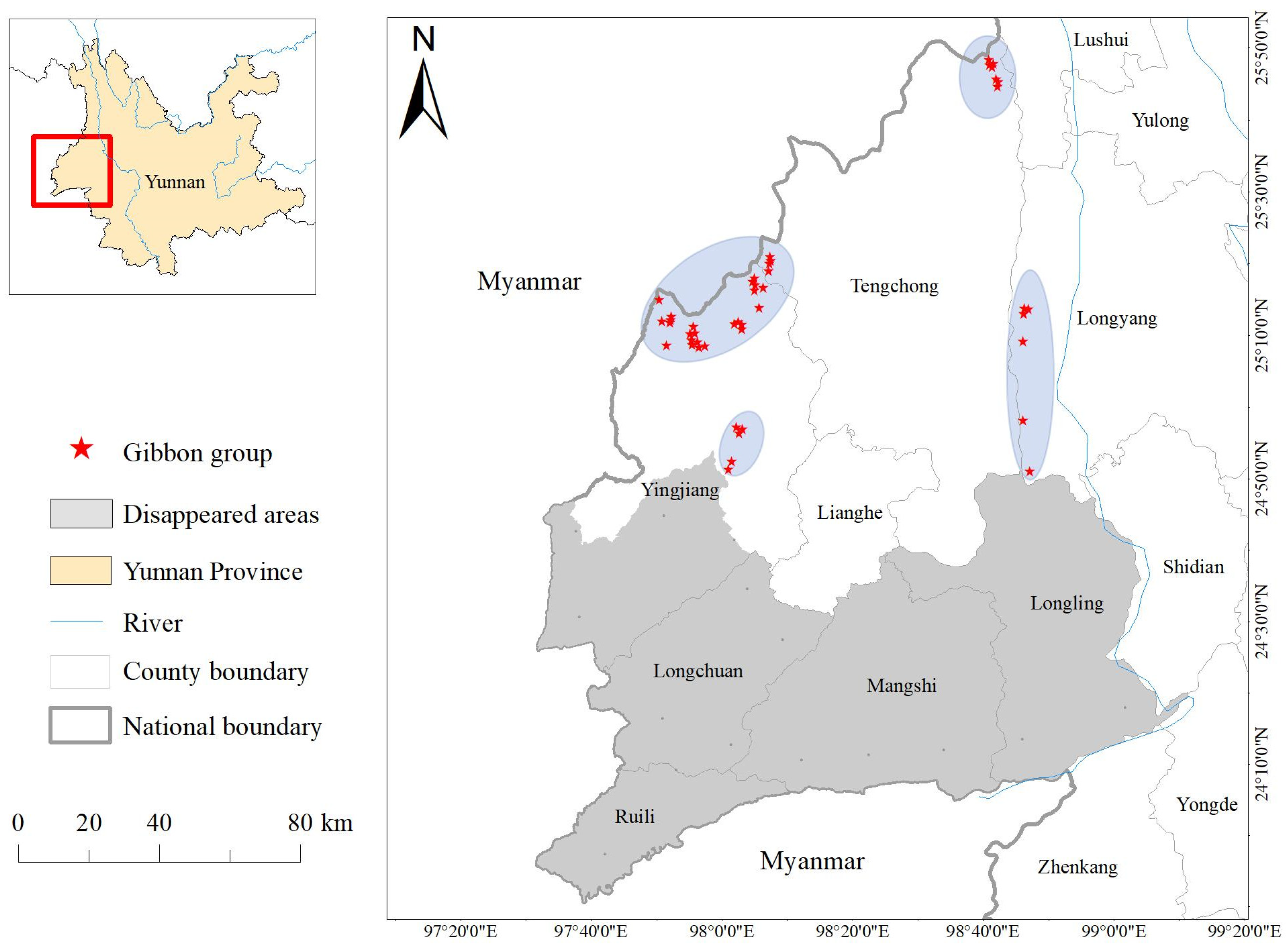
2.1. Study Site
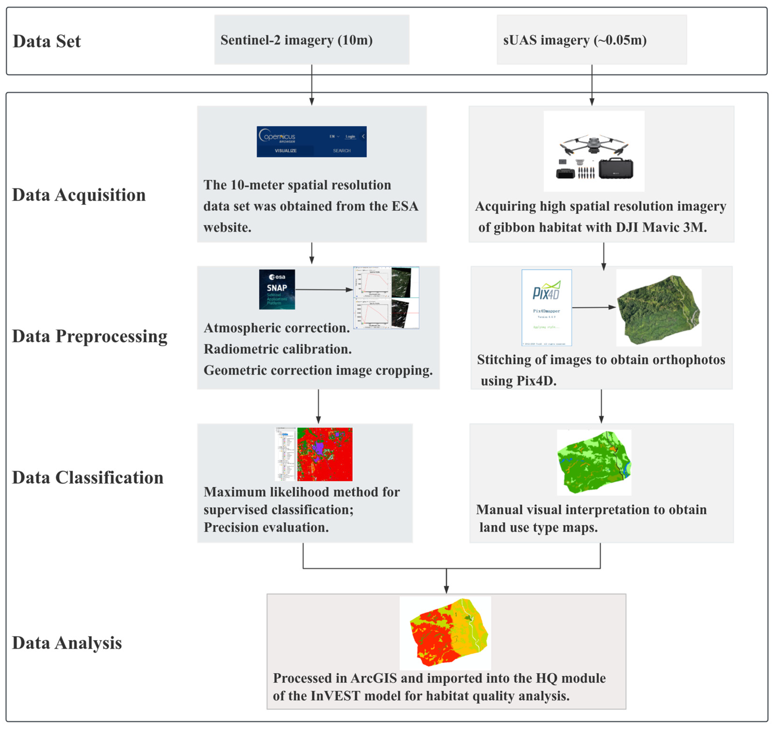
2.2. sUAS Data Acquisition and Processing
2.2.1. Data Acquisition
2.2.2. sUAS Data Preprocessing
2.3. Collection and Processing of Sentinel-2 Satellite Images
2.3.1. Data Collection
2.3.2. Satellite Image Preprocessing
2.4. Habitat Quality Assessment Based on the InVEST Model
3. Results
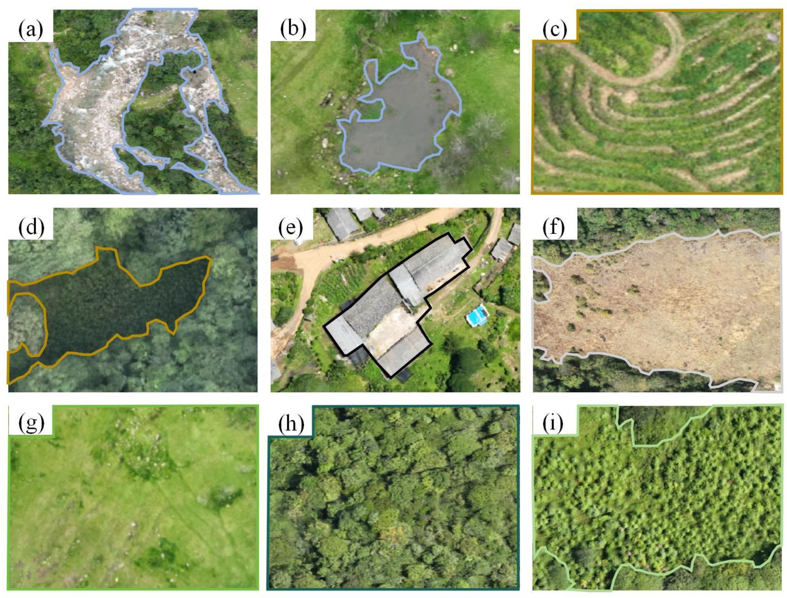
3.1. sUAS Survey in Gaoligong Hoolock Gibbon Habitat in Yingjiang
3.2. Classification Accuracy Assessment
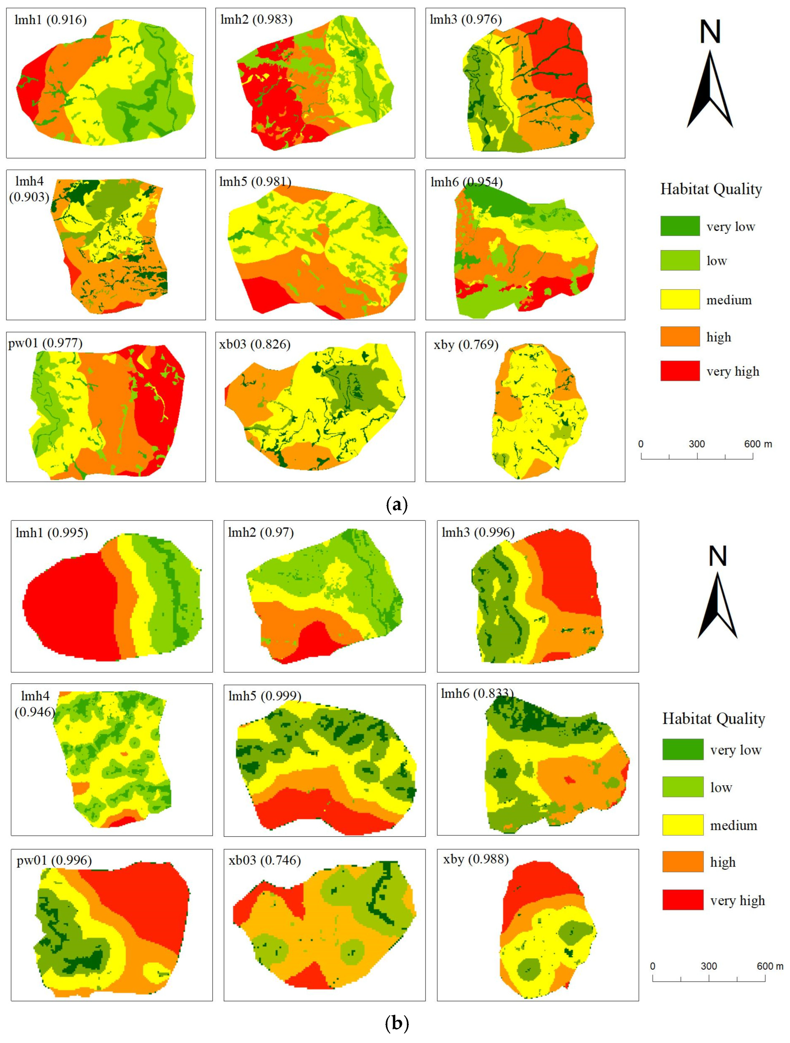
3.3. Habitat Quality Assessment Based on sUAS Images
3.4. Significant Impact of Image Resolution on Habitat Quality and Degradation Level Assessment and Difference Analysis
4. Discussion
4.1. sUAS Imaging Technique in Analysis of Gaoligong Hoolock Gibbon Habitat Patch Quality
4.2. Effects of Spatial Resolution on Classification Accuracy and Habitat Quality Analysis
4.3. Advantages of sUAS Imagery in Animal Habitat Analysis
5. Conclusions
Author Contributions
Funding
Data Availability Statement
Acknowledgments
Conflicts of Interest
Appendix A
References
- Estrada, A.; Garber, P.A.; Rylands, A.B. Impending extinction crisis of the world’s primates: Why primates matter. Sci. Adv. 2017, 3, e1600946. [Google Scholar] [CrossRef] [PubMed]
- Whittaker, D.J.; Lappan, S. The Gibbons: New Perspectives on Small Ape Socioecology and Population Biology; Springer International Publishing: New York, NY, USA, 2009; pp. 3–10. [Google Scholar]
- D’Agostino, J.; Cunningham, C. Preliminary investigation of flexibility in learning color reward associations in gibbons (Hylobatidae). Am. J. Primatol. 2015, 77, 854–868. [Google Scholar] [CrossRef] [PubMed]
- Fan, P.F.; He, K.; Chen, X. Description of a new species of Hoolock gibbon (Primates: Hylobatidae) based on integrative taxonomy. Am. J. Primatol. 2017, 79, e22631. [Google Scholar] [CrossRef] [PubMed]
- Wei, F.W.; Yang, Q.S.; Yi, W. Catalogue of mammals in China. Acta Theriol. Sin. 2021, 41, 487–501. [Google Scholar]
- Fan, P.F.; Turvey, S.T.; Bryant, J.V. Hoolock Tianxing (Amended Version of 2019 Assessment); The IUCN Red List of Threatened Species; International Union for Conservation of Nature: Gland, Switzerland, 2020; p. e.T118355648A166597159. [Google Scholar]
- Fan, P.F.; Wen, X.; Sheng, H. Distribution and conservation status of the Vulnerable eastern hoolock gibbon Hoolock leuconedys in China. Oryx 2011, 45, 129–134. [Google Scholar]
- Fan, P.F. Taxonomy and conservation status of gibbons in China. Acta Theriol. Sin. 2012, 32, 248–258. [Google Scholar]
- Zhou, Y.; Zhang, P. Distribution and vicissitude of gibbons (Hylobatidae) in China during the last 500 years. Acta Theriol. Sin. 2013, 33, 258–266. [Google Scholar]
- Yu, W.H.; He, K.L.; Fan, P.F. Progress in the classification and systematic evolution of Chinese veterinary species. J. Vet. Sci. 2021, 41, 502–524. [Google Scholar]
- Turvey, S.; Crees, J.; Di, F.M. Historical data as a baseline for conservation: Reconstructing long-term faunal extinction dynamics in Late Imperial-modern China. Proceedings. Biological sciences. R. Soc. 2015, 282, 20151299. [Google Scholar]
- Guan, Z.H.; Jiang, X.L. Population Status and Conservation Needs of the Endangered Hoolock tianxing in China. Oryx 2025, submitted.
- Li, Z.X.; Lin, Z.Y. Classification and distribution of living primates in Yunnan. China Zool. Res. 1983, 4, 111–120. [Google Scholar]
- Yang, D.; Zhang, J.; Li, C. A survey report on the number and distribution of gibbons in Yunnan. Med. Biol. Res. 1985, 3, 22–27. [Google Scholar]
- Ma, S.L.; Wang, Y.X. The recent distribution, status and conservation of primates in China. Acta Theriol. Sin. 1988, 8, 250–260. [Google Scholar]
- Lan, D.Y.; Ma, S.L.; Han, L. Distribution, Population Size and Conservation of Hoolock gibbons in West Yunnan; Chinese Forestry Publishing House: Beijing, China, 1995; pp. 11–19. [Google Scholar]
- Zhang, L.; Guan, Z.H.; Fei, H.L. Influence of traditional ecological knowledge on conservation of the Gaoligong hoolock gibbon (Hoolock tianxing) outside nature reserves. Biol. Conserv. 2020, 241, 108267. [Google Scholar] [CrossRef]
- Fan, P.F.; Ren, G.P.; Wang, W.; Scott, M.; Ma, C.Y. Habitat evaluation and population viability analysis of the last population of cao vit gibbon (Nomascus nasutus): Implications for conservation. Biol. Conserv. 2013, 161, 39–47. [Google Scholar] [CrossRef]
- Fan, P.F.; Ai, H.S.; Fei, H.L.; Zhang, D.; Yuan, S.-D. Seasonal variation of diet and time budget of Eastern hoolock gibbons (Hoolock leuconedys) living in a northen montane forest. Primates 2013, 54, 137–146. [Google Scholar] [CrossRef]
- Zhang, D.; Fei, H.L.; Yuan, S.D.; Sun, W.M.; Ni, Q.Y.; Cui, L.W.; Fan, P.F. Ranging behavior of eastern hoolock gibbon (Hoolock leuconedys) in a northern montane forest in Gaoligongshan, Yunnan, China. Primates 2013, 55, 239–247. [Google Scholar] [CrossRef]
- Ostapowicz, K.; Vogt, P.; Riitters, K.; Kozak, J.; Estreguil, C. Impact of scale on morphological spatial pattern of forest. Landsc. Ecol. 2008, 23, 1107–1117. [Google Scholar] [CrossRef]
- Qian, Y.G.; Zhou, W.Q.; Yu, W.J.; Pickett, S.T. Quantifying spatiotemporal pattern of urban greenspace: New insights from high resolution data. Landsc. Ecol. 2015, 30, 1165–1173. [Google Scholar] [CrossRef]
- Dungan, J.L.; Perry, J.N.; Dale, M.; Legendre, P.; Citron-Pousty, S.; Fortin, M.J. A balanced view of scale in spatial statistical analysis. Ecography 2002, 25, 626–640. [Google Scholar] [CrossRef]
- Gurevitch, J.; Scheiner, S.; Fox, G.A. The Ecology of Plants. In Landscapes: Pattern and Scale; Oxford University Press: Oxford, UK, 2023. [Google Scholar]
- Wasserman, T.; Sánchez, M.; Andrew; Waltz, A. Grain and Extent Considerations Are Integral for Monitoring Landscape-Scale Desired Conditions in Fire-Adapted Forests. Forests 2019, 10, 465. [Google Scholar] [CrossRef]
- Guisan, A.; Elith, J.; Graham, C.; Phillips, S.; Peterson, A.; Zimmermann, N. What matters for predicting spatial distributions of trees: Techniques, data, or species’ characteristics? Ecol. Monogr. 2007, 77, 615–630. [Google Scholar] [CrossRef]
- Yann, B.C.; Pauline, S.; André, D. Importance of high-resolution spatial data for the detection of winter wildlife responses to edges. Can. J. For. Res. 2024, 54, 816–824. [Google Scholar]
- Fletcher, R.; Betts, M.G.; Damschen, E.I.; Hefey, T.J.; Hightower, J.; Smith, T.A.H.; Fortin, M.; Haddad, N.M. Addressing the problem of scale that emerges with habitat fragmentation. Glob. Ecol. Biogeogr. 2023, 32, 828–841. [Google Scholar] [CrossRef]
- Kong, F.; Yin, H.; James, P.; Hutyra, L.R.; He, H.S. Efects of spatial pattern of greenspace on urban cooling in a large metropolitan area of eastern China. Landsc. Urban Plan. 2014, 128, 35–47. [Google Scholar] [CrossRef]
- Wiens, J. A Spatial Scaling in ecology. Funct. Ecol. 1989, 3, 385–397. [Google Scholar] [CrossRef]
- Lawler, J.; O’Connor, R.; Hunsaker, C.; Jones, K.; Loveland, T.; White, D. The Effects of Habitat Resolution on Models of Avian Diversity and Distributions: A Comparison of Two Land-Cover Classifications. Landsc. Ecol. 2004, 19, 515–530. [Google Scholar] [CrossRef]
- Tian, P.; Cao, L.D.; Li, J.L.; Pu, R.L.; Shi, X.L.; Wang, L.J.; Liu, R.Q. Landscape Grain Effect in Yancheng Coastal Wetland and Its Response to Landscape Changes. Int. J. Environ. Res. Public Health 2019, 16, 2225. [Google Scholar] [CrossRef]
- Masoudi, M.; Richards, D.; Puay, Y.T. Assessment of the Influence of Spatial Scale and Type of Land Cover on Urban Landscape Pattern Analysis Using Landscape Metrics. J. Geovisualization Spat. Anal. 2024, 8, 10. [Google Scholar] [CrossRef]
- Kerr, J.; Ostrovsky, M. From space to species: Ecological applications for remote sensing. Trends Ecol. Evol. 2003, 18, 299–305. [Google Scholar] [CrossRef]
- Newton, A.; Hill, R.; Echeverría, C.; Golicher, D.; Benayas, J.; Cayuela, L.; Hinsley, S. Remote sensing and the future of landscape ecology. Prog. Phys. Geogr. 2009, 33, 528–546. [Google Scholar] [CrossRef]
- Lepczyk, C.; Wedding, L.; Asner, G.; Pittman, S.; Goulden, T.; Linderman, M.; Gang, J.; Wright, R. Advancing Landscape and Seascape Ecology from a 2D to a 3D Science. BioScience 2021, 71, 596–608. [Google Scholar] [CrossRef]
- O’Connell, J.R.; Glass, A.; Crawford, C.S.; Eichholz, M.W. Efficacy of Mapping Grassland Vegetation for Land Managers and Wildlife Researchers Using sUAS. Drones 2022, 6, 318. [Google Scholar] [CrossRef]
- Scheeres, J.; de Jong, J.; Brede, B.; Brancalion, P. Distinguishing forest types in restored tropical landscapes with UAV-borne LIDAR. Remote Sens. Environ. 2023, 290, 113533. [Google Scholar] [CrossRef]
- Mangewa, L.; Ndakidemi, P.; Alward, R.; Kija, H.; Bukombe, J.; Nasolwa, E.; Munishi, L. Comparative Assessment of UAV and Sentinel-2 NDVI and GNDVI for Preliminary Diagnosis of Habitat Conditions in Burunge Wildlife Management Area, Tanzania. Earth 2022, 3, 769–787. [Google Scholar] [CrossRef]
- Li, S.S.; Wang, G.J.; Zhang, H.; Zou, Y.H. Observing Individuals and Behavior of Hainan Gibbons (Nomascus hainanus) Using Drone Infrared and Visible Image Fusion Technology. Drones 2023, 7, 543. [Google Scholar] [CrossRef]
- Madurapperuma, B. Unmanned aerial vehicles in wildlife research: A review for future research need in Sri Lanka. In Proceedings of the WILDLANKA International Symposium, Colombo, Sri Lanka, 7–9 August 2018. [Google Scholar]
- Linchant, J.; Lejeune, P.; Quevauvillers, S.; Vermeulen, C.; Brostaux, Y.; Lhoest, S.; Michez, A. Evaluation of an Innovative Rosette Flight Plan Design for Wildlife Aerial Surveys with UAS. Drones 2023, 7, 208. [Google Scholar] [CrossRef]
- Yan, N.; Dai, X.H.; Wang, B.; Wen, M.C. Mapping potential human-elephant conflict hotspots with UAV monitoring data. Glob. Ecol. Conserv. 2023, 43, e02451. [Google Scholar]
- Francis, R.J.; Brandis, K.J. Assessment of Ground and Drone Surveys of Large Waterbird Breeding Rookeries: A Comparative Study. Drones 2024, 8, 135. [Google Scholar] [CrossRef]
- Li, H.; Li, R. Plant Resources and Phylogeography of the Gaoligong Mountains; Hubei Science and Technology Press: Wuhan, China, 2020. [Google Scholar]
- PIX4Dmapper. Available online: https://www.pix4d.com/product/pix4dmapper-photogrammetry-software/ (accessed on 7 December 2023).
- Louis, J.; Pflug, B.; Pertiwi, A.; Pignatale, F.; Enache, S.; Iannone, R.; Boccia, V. Sentinel-2 Level-2 processing Sen2Cor status and outlook of 2022. In Proceedings of the 6th International Symposium on Recent Advances in Quantitative Remote Sensing: RAQRS’VI, Valencia, Spain, 19–23 September 2022. [Google Scholar]
- Sharma, R.; Ghosh, A.; Joshi, P. Decision tree approach for classification of remotely sensed satellite data using open source support. J. Earth Syst. Sci. 2013, 122, 1237–1247. [Google Scholar] [CrossRef]
- Huang, K.; Dai, W.Y.; Huang, W.L.; Ou, H.; Hu, H.X. Impacts of land use change evaluation on habitat quality based on CA-Markov and InVEST model, Bullet. Soil Water Conserv. 2019, 39, 155–162. [Google Scholar]
- Sharp, R.; Tallis, H.T.; Ricketts, T. InVEST 3.3.0 User’s Guide, the Natural Capital Project; Stanford University: Stanford, CA, USA; University of Minnesota: Minneapolis, MN, USA, 2016. [Google Scholar]
- Esri. ArcGISDesktop. Version10.8. 2020. Available online: https://www.esri.com/en-us/arcgis/products/arcgis-pro/overview (accessed on 11 April 2021).
- Liang, X.; Yuan, L.; Ning, L.; Song, C.; Cheng, C.; Wang, X. Spatial pattern and influencing factors of habitat quality in Heilongjiang Province based on InVEST model. J. Beijing Norm. Univ. Nat. Sci. Ed. 2020, 56, 864–872. [Google Scholar]
- Shi, J.; Liang, X.; Li, H.; Wei, Z. Impact of landscape pattern on ecosystem service trade-offs in the Loess Plateau of Northern Shaanxi. Acta Ecol. Sin. 2023, 43, 8958–8972. [Google Scholar]
- Marsh, L. Primates in Fragments: Ecology and Conservation; Springer: New York, NY, USA, 2003. [Google Scholar]
- Salmaniw, Y.; Shen, Z.; Wang, H. From habitat decline to collapse: A spatially explicit approach connecting habitat degradation to destruction. arXiv 2024, arXiv:2403.11200. [Google Scholar]
- Luan, Y.; Huang, G.; Zheng, G.; Wang, Y. Correlation between Spatio-Temporal Evolution of Habitat Quality and Human Activity Intensity in Typical Mountain Cities: A Case Study of Guiyang City, China. Int. J. Environ. Res. Public Health 2022, 19, 14294. [Google Scholar] [CrossRef]
- Istiadi, Y.; Priatna, D.; Widodo, W. Analysis of the Edge Effect on Bird And Primate Distribution in the Ecological Corridor Habitat of Mount Halimun Salak National Park (TNGHS). Eduvest 2024, 4, 4104–4110. [Google Scholar] [CrossRef]
- Bai, B.; Zhou, W.; Ai, H.S.; LI, Z.B.; Zhang, X.Y.; Hu, C.G. Habitat Use of the Hoolock Gibbon (Hoolock hoolock) at Nankang, Mt. Gaoligong in Spring. Zool. Res. 2007, 28, 179–185. [Google Scholar]
- Fan, P.F.; Bartlett, T. Overlooked small apes need more attention! Am. J. Primatol. 2017, 79, e22658. [Google Scholar] [CrossRef]
- Yuan, S.D.; Fei, H.L.; Zhu, S.H.; Cui, L.W.; Ai, H.S.; Fan, P.F. Effects of tsaoko (Fructus tsaoko) cultivating on tree diversity and canopy structure in the habitats of eastern hoolock gibbon (Hoolock leuconedys). Zool. Res. 2014, 35, 231–239. [Google Scholar]
- Aung, P.P.; Lwin, N.; Aung, T.; Soe, M.H.; Thompson, C. Confirmation of Gaoligong Hoolock Gibbon (Hoolock tianxing) in Myanmar Extends Known Geographic Range of an Endangered Primate. Int. J. Primatol. 2024, 45, 1–24. [Google Scholar] [CrossRef]
- Awuah, T.K. Effects of Spatial Resolution, Land-Cover Heterogeneityand Different Classification Methods on Accuracy of Land-Cover Mapping; SLU University Library: St. Louis, MO, USA, 2018. [Google Scholar]
- Lin, J.Y.; Zeng, Y.Z.; He, Y.Q. Spatial Optimization with Morphological Spatial Pattern Analysis for Green Space Conservation Planning. Forests 2023, 14, 1031. [Google Scholar] [CrossRef]
- Huang, X.Y.; Zhang, Z.Y.; Ye, J.G.; Gao, J. A township-level assessment of forest fragmentation using morphological spatial pattern analysis in Qujing. J. Mt. Sci. 2021, 18, 3125–3137. [Google Scholar] [CrossRef]
- Kattenborn, T.; Lopatin, J.; Förster, M.; Braun, A.; Fassnacht, F. UAV data as alternative to field sampling to map woody invasive species based on combined Sentinel-1 and Sentinel-2 data. Remote Sens. Environ. 2019, 227, 61–73. [Google Scholar] [CrossRef]
- Varol, B.; Szabo, S.; Topaloğlu, R.; Bozbay, G.; Sertel, E. Analysis of the association between image resolution and landscape metrics using multi-sensor LULC maps. J. Environ. Plan. Manag. 2023, 67, 2281–2302. [Google Scholar] [CrossRef]
- Silveyra, G.R.; Latifi, H.; Weinacker, H.; Dees, M.; Koch, B.; Heurich, M. Integrating LiDAR and high-resolution imagery for object-based mapping of forest habitats in a heterogeneous temperate forest landscape. Int. J. Remote Sens. 2018, 39, 8859–8884. [Google Scholar] [CrossRef]
- Santecchia, G.S.; Delrieux, C. Automatic Land Use Classification in High-Resolution RGB Images. In Proceedings of the 2024 L Latin American Computer Conference (CLEI), Buenos Aires, Argentina, 12–16 August 2024; pp. 1–11. [Google Scholar]
- Corry, R.; Nassauer, J. Limitations of using landscape pattern indices to evaluate the ecological consequences of alternative plans and designs. Landsc. Urban Plan. 2006, 72, 265–280. [Google Scholar] [CrossRef]
- Jurišić, M.; Radočaj, D.; Plaščak, I.; Rapčan, I. A UAS and Machine Learning Classification Approach to Suitability Prediction of Expanding Natural Habitats for Endangered Flora Species. Remote Sens. 2022, 14, 3054. [Google Scholar] [CrossRef]
- Zhu, Y.L.; Xu, M.L.; Zhang, L.X.; Li, P.; Jin, B.; Zuo, A.R.; Jiang, X.L.; Guan, Z.H. Prediction of the potential dispersal corridors for Gaoligong hoolock gibbon in northern Yingjiang, Yunnan, China. J. Nat. Conserv. 2024, 83, 126771. [Google Scholar] [CrossRef]
- Wang, Z.; Liu, R.; Liu, Q.R.; Han, L.C. Towards Reliable UAV-Enabled Positioning in Mountainous Environments: System Design and Preliminary Results. IEEE Trans. Reliab. 2022, 71, 1435–1463. [Google Scholar] [CrossRef]
- Bishop, M.P.; Bagavathiannan, M.V.; Cope, D.; Huo, D.; Murray, S.C.; Olsenholler, J.A.; Rooney, W.L.; Thomasson, J.A.; Valasek, J.; Young, B.W.; et al. High-Resolution UAS Imagery in Agricultural Research Concepts, Issues, and Research Directions; CRC Press: Boca Raton, FL, USA, 2018; pp. 3–32. [Google Scholar]


| Village Name | Patch Name |
|---|---|
| lamahe | lmh1 |
| lmh2 | |
| lmh3 | |
| lmh4 | |
| lmh5 | |
| lmh6 | |
| pawa | pw01 |
| xiangbai | xb03 |
| xinbaiyan | xby |
| Threat | Max_Dist | Weight | Decay |
|---|---|---|---|
| residential buildings | 1 | 1 | exponential |
| bare ground | 0.6 | 0.5 | linear |
| cropland | 0.4 | 0.4 | linear |
| sod | 0.3 | 0.3 | linear |
| waterbody | 0.2 | 0.2 | linear |
| coniferous | 0.1 | 0.2 | linear |
| LULC | Habitat Suitability | Residential Buildings | Bare Ground | Cropland | Sod | Waterbody | Coniferous |
|---|---|---|---|---|---|---|---|
| no data | 0 | 0 | 0 | 0 | 0 | 0 | 0 |
| grass | 0.4 | 0.4 | 0.5 | 0.3 | 1 | 0.5 | 0.6 |
| pine forest | 0.7 | 0.6 | 0.7 | 0.6 | 0.6 | 0.5 | 1 |
| farm | 0.2 | 0.3 | 0.4 | 1 | 0.5 | 0.4 | 0.6 |
| forest | 1 | 0.9 | 0.8 | 0.8 | 0.7 | 0.6 | 0.3 |
| water | 0.5 | 0.7 | 0.6 | 0.5 | 0.6 | 1 | 0.5 |
| bare | 0 | 0.4 | 1 | 0.4 | 0.4 | 0.4 | 0.7 |
| built-up | 0 | 1 | 0.4 | 0.4 | 0.6 | 0.2 | 0.8 |
| Forest | Grass | Farm | Bare | Pine Forest | Built-Up | Water | |
|---|---|---|---|---|---|---|---|
| xby | 91.53% | 0.94% | 5.12% | 0.33% | 2.08% | 0.01% | 0% |
| pw01 | 87.92% | 6.25% | 2.16% | 0% | 2.20% | 0.86% | 0.61% |
| xb03 | 84.87% | 3.55% | 5.88% | 1.51% | 1.09% | 0% | 0% |
| lmh5 | 84.51% | 12.50% | 0.57% | 1.00% | 1.42% | 0% | 0% |
| lmh1 | 79.22% | 4.73% | 4.69% | 3.78% | 5.00% | 2.21% | 0.36% |
| lmh3 | 77.21% | 6.98% | 5.37% | 0.72% | 6.06% | 1.94% | 1.71% |
| lmh4 | 70.70% | 15.57% | 3.99% | 8.96% | 0.77% | 0% | 0% |
| lmh2 | 67.77% | 21.98% | 2.22% | 0.05% | 5.43% | 0.89% | 1.67% |
| lmh6 | 62.68% | 19.76% | 12.15% | 0.74% | 3.88% | 0.54% | 0.25% |
| Forest | Grass | Farm | Built-Up | Bare | Water | Producer’s Accuracy/% | |
|---|---|---|---|---|---|---|---|
| Forest | 215 | 0 | 0 | 0 | 21 | 5 | 100 |
| Grass | 0 | 70 | 26 | 8 | 4 | 0 | 93.33 |
| Farm | 0 | 4 | 21 | 9 | 8 | 11 | 17.36 |
| Built-up | 0 | 1 | 43 | 59 | 0 | 73 | 77.63 |
| Bare | 0 | 0 | 31 | 0 | 2 | 0 | 5.71 |
| Water | 0 | 0 | 0 | 0 | 0 | 11 | 11 |
| User’s Accuracy/% | 89.21 | 64.81 | 39.62 | 33.52 | 6.06 | 100 | |
| Overall accuracy | 60.77% | ||||||
| Kappa coefficient | 0.5023 | ||||||
| Habitat Quality | Current Level of Degradation | |||
|---|---|---|---|---|
| sUAS (0.05 m) | Sentinel-2 (10 m) | sUAS (0.05 m) | Sentinel-2 (10 m) | |
| average | 0.92 | 0.94 | 0.68 | 0.76 |
Disclaimer/Publisher’s Note: The statements, opinions and data contained in all publications are solely those of the individual author(s) and contributor(s) and not of MDPI and/or the editor(s). MDPI and/or the editor(s) disclaim responsibility for any injury to people or property resulting from any ideas, methods, instructions or products referred to in the content. |
© 2025 by the authors. Licensee MDPI, Basel, Switzerland. This article is an open access article distributed under the terms and conditions of the Creative Commons Attribution (CC BY) license (https://creativecommons.org/licenses/by/4.0/).
Share and Cite
Xu, M.; Zhu, Y.; Zhang, L.; Li, P.; Gong, Q.; Zuo, A.; Hu, K.; Jiang, X.; Lu, N.; Guan, Z. sUAS-Based High-Resolution Mapping for the Habitat Quality Assessment of the Endangered Hoolock tianxing Gibbon. Forests 2025, 16, 285. https://doi.org/10.3390/f16020285
Xu M, Zhu Y, Zhang L, Li P, Gong Q, Zuo A, Hu K, Jiang X, Lu N, Guan Z. sUAS-Based High-Resolution Mapping for the Habitat Quality Assessment of the Endangered Hoolock tianxing Gibbon. Forests. 2025; 16(2):285. https://doi.org/10.3390/f16020285
Chicago/Turabian StyleXu, Mengling, Yongliang Zhu, Lixiang Zhang, Peng Li, Qiangbang Gong, Anru Zuo, Kunrong Hu, Xuelong Jiang, Ning Lu, and Zhenhua Guan. 2025. "sUAS-Based High-Resolution Mapping for the Habitat Quality Assessment of the Endangered Hoolock tianxing Gibbon" Forests 16, no. 2: 285. https://doi.org/10.3390/f16020285
APA StyleXu, M., Zhu, Y., Zhang, L., Li, P., Gong, Q., Zuo, A., Hu, K., Jiang, X., Lu, N., & Guan, Z. (2025). sUAS-Based High-Resolution Mapping for the Habitat Quality Assessment of the Endangered Hoolock tianxing Gibbon. Forests, 16(2), 285. https://doi.org/10.3390/f16020285