
LAI Mapping of Winter Moso Bamboo Forests Using Zhuhai-1 Hyperspectral Images and a PSO-SVM Model

 ,
,  and
and
Abstract
:1. Introduction
2. Materials and Methods
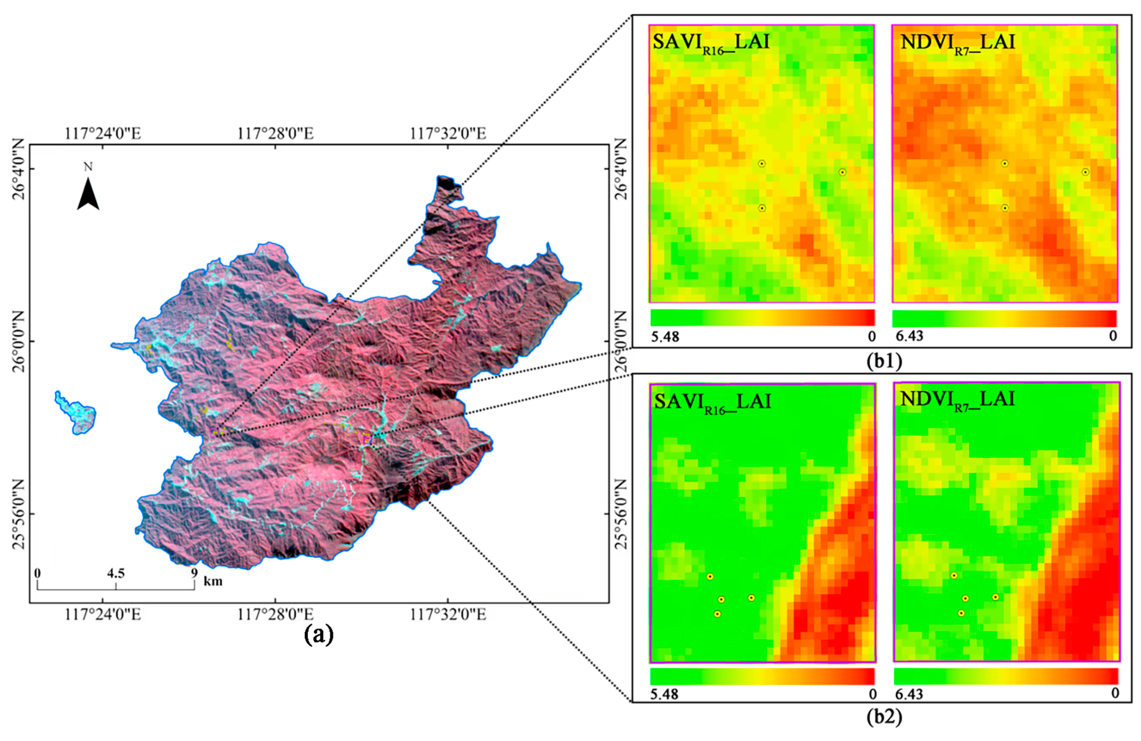
2.1. Study Area
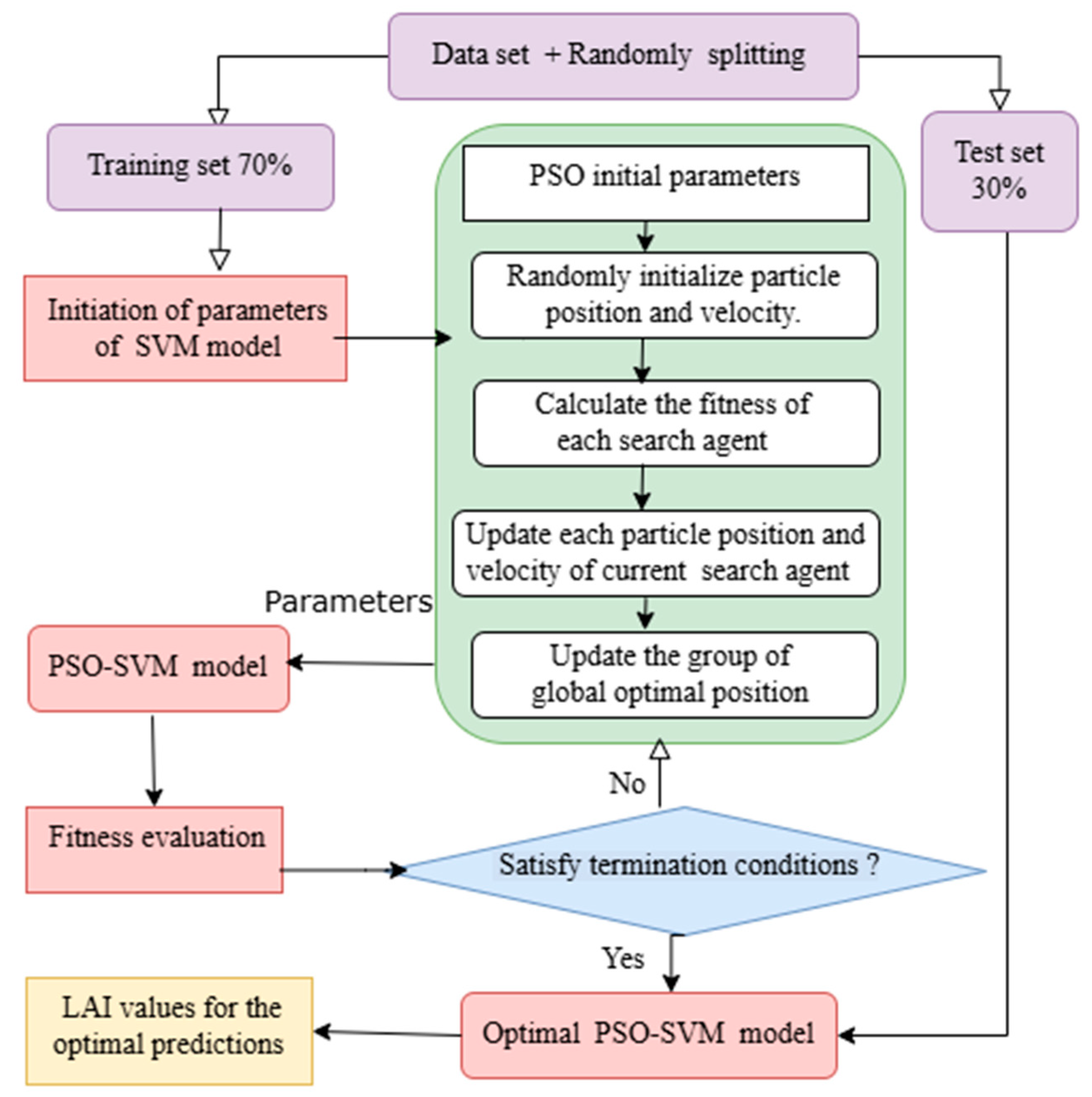
2.2. Study Workflow
2.3. Data Acquisition and Preparation
2.3.1. Field Measurements
2.3.2. Zhuhai-1 Orbit Hyperspectral Images Acquisition and Preprocessing
2.3.3. Hyperspectral Vegetation Index Extraction
2.4. Model Construction Between VIs and LAI of MBFs
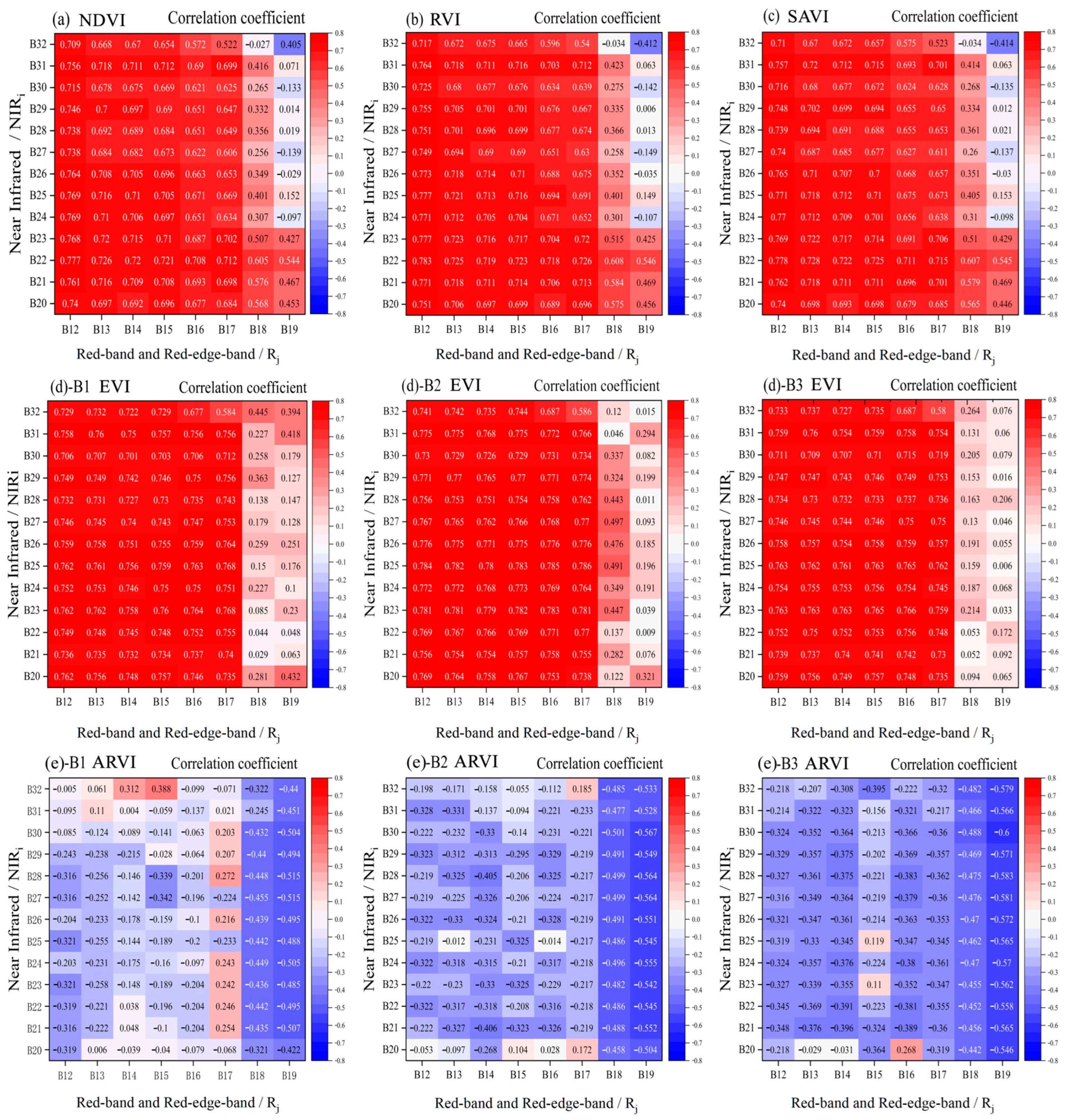
2.4.1. Model Variable Screening Method Using Correlation Analysis
2.4.2. Constructing LAI Models Using the Empirical Statistical Method Based on Single-VI
2.4.3. Constructing LAI Models by Combining Machine-Learning Algorithms with Hyperspectral VIs
SVM and PSO-SVM Machine-Learning Algorithms
RF, PLSR, and XGBoost Algorithms
2.5. Model Evaluation
3. Results
3.1. Screening VIs to Estimate the LAI of MBFs
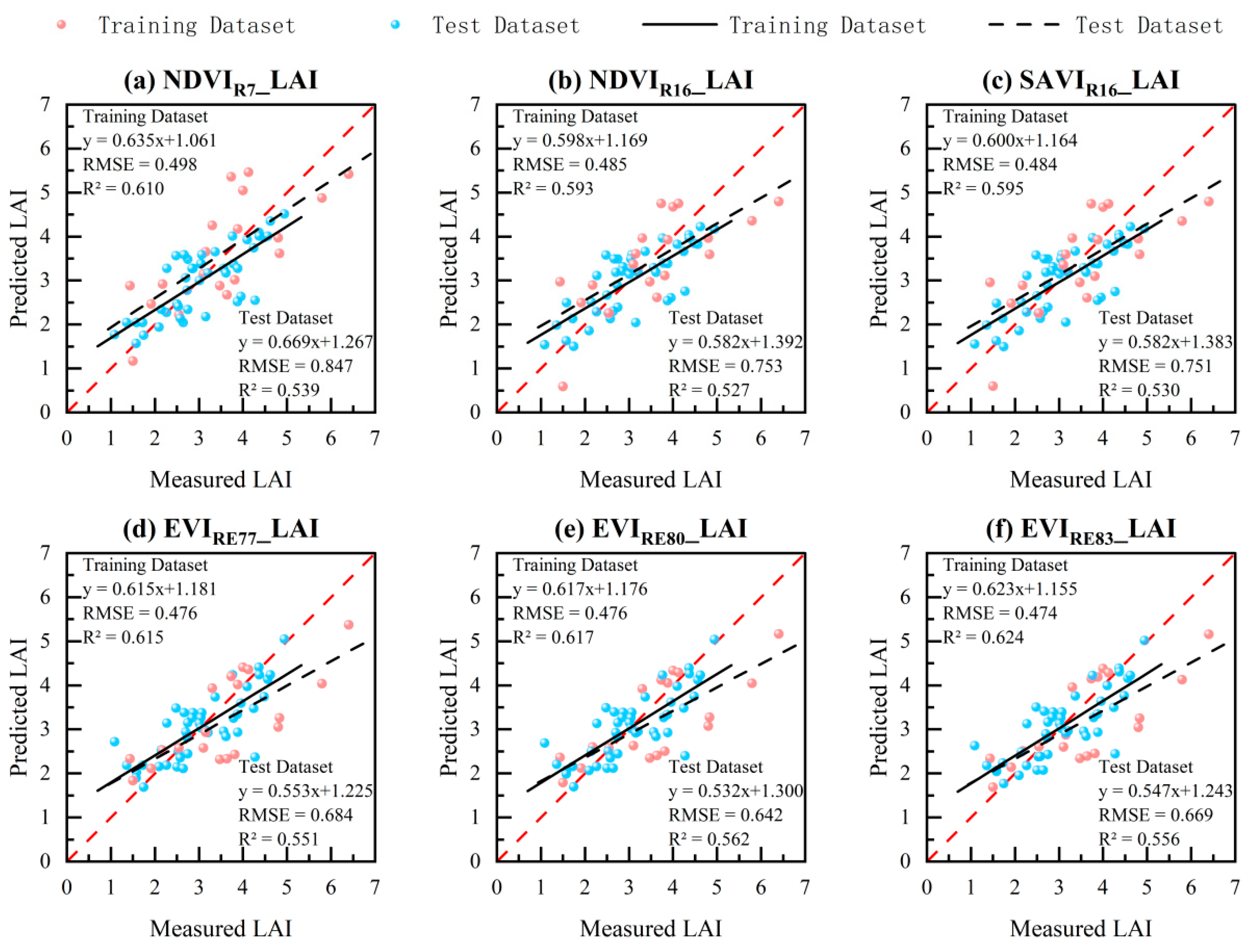
3.2. Univariate Empirical Model Construction and Selection for LAI Estimation
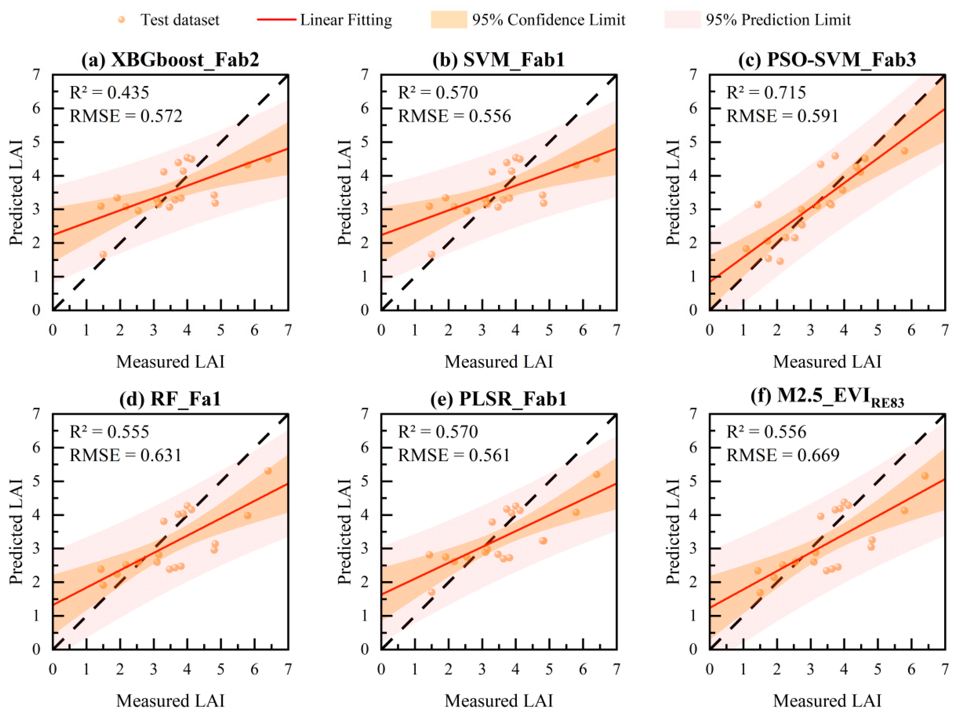
3.3. Machine-Learning Model Based on Multivariate VIs
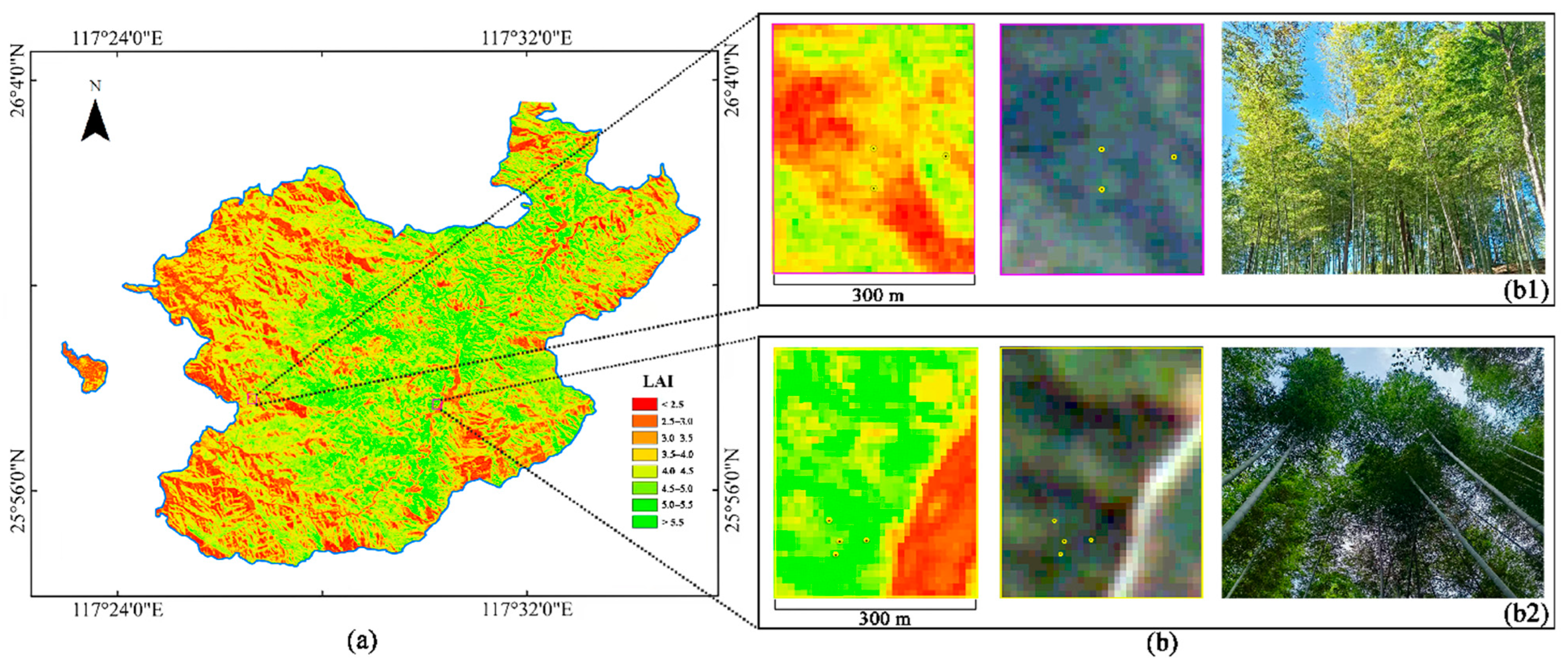
3.4. Model Evaluation and LAI Mapping for Moso Bamboo in the Winter Growth Stage
4. Discussion
4.1. Effect of Hyperspectral VI on LAI Estimation
4.2. Measures of Modeling LAI in Empirical and Machine-Learning Models
4.3. LAI Values and Management Implications for MBFs
4.4. Limitations and Scope for Future Studies
5. Conclusions
Author Contributions
Funding
Data Availability Statement
Conflicts of Interest
References
- Peng, Y.; Li, Y.; Dai, C.; Fang, S.H.; Gong, Y.; Wu, X.T.; Zhu, R.S.; Liu, K. Remote prediction of yield based on LAI estimation in oilseed rape under different planting methods and nitrogen fertilizer applications. Agric. For. Meteorol. 2019, 271, 116–125. [Google Scholar] [CrossRef]
- Ji, J.; Li, X.; Du, H.; Mao, F.; Fan, W.; Xu, Y.; Huang, Z.; Wang, J.; Kang, F. Multiscale leaf area index assimilation for Moso bamboo forest based on Sentinel-2 and MODIS data. J. Appl. Geogr. 2021, 102, 102519. [Google Scholar] [CrossRef]
- Qin, Z.; Yang, H.; Shu, Q.; Yu, J.; Xu, L.; Wang, M.; Xia, C.; Duan, D. Estimation of leaf area index for Dendrocalamus giganteus based on multi-source remote sensing data. Forests 2024, 15, 1257. [Google Scholar] [CrossRef]
- Weiss, M.; Jacob, F.; Duveiller, G. Remote sensing for agricultural applications: A meta-review. Remote Sens. Environ. 2020, 236, 111402. [Google Scholar] [CrossRef]
- Liang, L.; Geng, D.; Yan, J.; Qiu, S.; Di, L.; Wang, S.; Xu, L.; Wang, L.; Kang, J.; Li, L. Estimating crop LAI using spectral feature extraction and the hybrid inversion method. Remote Sens. 2020, 12, 3534. [Google Scholar] [CrossRef]
- Cao, L.; Coops, N.C.; Sun, Y.; Ruan, H.; She, G. Estimating canopy structure and biomass in bamboo forests using airborne lidar data. ISPRS J. Photogramm. Remote Sens. 2019, 148, 114–129. [Google Scholar] [CrossRef]
- Li, D.; Wei, J.; Wu, J.; Zhong, Y.; Chen, Z.; He, J.; Zhang, S.; Yu, L. The expansion of Moso Bamboo (Phyllostachys edulis) foreinto diverse types of forests in China from 2010 to 2020. Forests 2024, 15, 1418. [Google Scholar] [CrossRef]
- Li, N.; Hu, M.Y.; Xie, J.Y.; Wei, L.J.; Wu, T.Z.; Zhang, W.; Gu, S.X.; Li, L.W. Enhancing aboveground biomass estimation in Moso bamboo forests: The role of on-year and off-year phenomena in remote sensing. Front. For. Glob. Change 2025, 8, 1515767. [Google Scholar] [CrossRef]
- Wang, T.; Skidmore, A.K.; Toxopeus, A.G.; Liu, X. Understory Bamboo Discrimination Using a Winter Image. Photogramm. Eng. Remote Sens. 2009, 75, 37–45. [Google Scholar] [CrossRef]
- Zou, J.; Hou, W.; Chen, L.; Wang, Q.; Zhong, P.; Zuo, Y.; Luo, S.; Leng, P. Evaluating the impact of sampling schemes on leaf area index measurements from digital hemispherical photography in Larix principis-rupprechtii forest plots. For. Ecosyst. 2020, 7, 686–703. [Google Scholar] [CrossRef]
- Xu, Z.; Lin, L.; Huang, X.; Liu, J.; Zhong, Z. Estimation model of Moso bamboo LAI and spatial distribution characteristics: A case in Shunchang county, Fujian province. J. Hainan Univ. (Nat. Sci. Ed.) 2018, 36, 9. [Google Scholar] [CrossRef]
- Yao, X.; Zeng, Q.; Liu, J.; Zhang, W.; Yu, K. High-Spectral Estimation of LAI in Moso Bamboo Stands. J. For. Environ. 2018, 38, 6. [Google Scholar] [CrossRef]
- Xu, X.; Du, H.; Zhou, G.; Mao, F.; Li, X.; Zhu, D.; Li, Y.; Cui, L. Remote estimation of canopy leaf area index and chlorophyll content in Moso bamboo (Phyllostachys edulis [Carrière] J. Houz.) forest using MODIS reflectance data. Ann. For. Sci. 2017, 75, 33. [Google Scholar] [CrossRef]
- Sun, H.; Ju, H.; Zhang, H.; Lin, H.; Ling, C. Comparison of three regression analysis methods for application to LAI inversion using Hyperion data. Acta Ecol. Sin. 2012, 32, 7781–7790. [Google Scholar] [CrossRef]
- Tamang, M.; Nandy, S.; Srinet, R.; Das, A.K.; Padalia, H. Bamboo mapping using earth observation data: A systematic review. J. Indian. Soc. Remote Sens. 2022, 50, 2055–2072. [Google Scholar] [CrossRef]
- Dong, T.; Liu, J.; Shang, J. Assessment of red-edge vegetation indices for crop leaf area index estimation. Remote Sens. Environ. 2019, 222, 133–143. [Google Scholar] [CrossRef]
- Wang, W.; Zhang, X.; Shang, K.; Feng, R.; Wang, Y.; Ding, S.; Xiao, Q. Estimation of soil organic matter content by combining Zhuhai-1 hyperspectral and Sentinel-2A multispectral images. Comput. Electron. Agric. 2024, 226, 109377. [Google Scholar] [CrossRef]
- Wang, X.; Lu, X.; Meng, Q.; Li, G.; Wang, J.; Zhang, L.; Yang, Z. Inversion of Leaf Area Index Based on GF-6 WFV spectral vegetation index model. Spectrosc. Spectr. Anal. 2022, 42, 2278–2283. [Google Scholar] [CrossRef]
- Sun, Y.; Wang, B.; Zhang, Z. Improving leaf area index estimation with chlorophyll insensitive multispectral red-edge vegetation indices. IEEE J. Sel. Top. Appl. Earth Obs. Remote Sens. 2023, 16, 3568–3582. [Google Scholar] [CrossRef]
- Zhang, Y.; Qi, T.; Sun, Y.; Qu, X.; Cao, Y.; Wu, M.; Liu, C.; Wang, L. Vegetation characteristics of GF-6 remote sensing image and its application on LAI retrieval of winter wheat seedling stage. Acta Agron. Sin. 2021, 47, 2532–2540. [Google Scholar]
- Qiao, K.; Zhu, W.; Xie, Z.; Wu, S.; Li, S. New three red-edge vegetation index (VI3RE) for crop seasonal LAI prediction using Sentinel-2 data. Int. J. Appl. Earth Obs. Geoinf. 2024, 130, 103894. [Google Scholar] [CrossRef]
- Wei, S.; Yin, T.; Yuan, B.; Ow, G.L.F.; Yusof, M.L.M.; Gastellu-Etchegorry, J.P.; Whittle, A. Estimation of chlorophyll content for urban trees from UAV hyperspectral images. Int. J. Appl. Earth Obs. Geoinf. 2024, 126, 103617. [Google Scholar] [CrossRef]
- Navarro-Cerrillo, R.M.; Trujillo, J.; de la Orden, M.S.; Hernández-Clemente, R. Hyperspectral and multispectral satellite sensors for mapping chlorophyll content in a Mediterranean Pinus sylvestris L. plantation. Int. J. Appl. Earth Obs. Geoinf. 2014, 26, 88–96. [Google Scholar] [CrossRef]
- Fan, J.; Liu, Y.; Fan, Y.; Yao, Y.; Chen, R.; Bian, M.; Ma, Y.; Wang, H.; Feng, H. Estimation of potato leaf area index based on spectral information and Haralick textures from UAV hyperspectral images. Front. Plant Sci. 2024, 15, 1492372. [Google Scholar] [CrossRef] [PubMed]
- Pascual-Venteo, A.B.; Portalés, E.; Berger, K.; Tagliabue, G.; Garcia, J.L.; Pérez-Suay, A.; Rivera-Caicedo, J.P.; Verrelst, J. Prototyping Crop Traits Retrieval Models for CHIME: Dimensionality Reduction Strategies Applied to PRISMA Data. Remote Sens. 2022, 14, 2448. [Google Scholar] [CrossRef] [PubMed]
- Chen, Z.; Jia, K.; Xiao, C.; Wei, D.; Zhao, X.; Lan, J.; Wei, X.; Yao, Y.; Wang, B.; Sun, Y.; et al. Leaf area index estimation algorithm for GF-5 hyperspectral data based on different feature selection and machine learning methods. Remote Sens. 2020, 12, 2110. [Google Scholar] [CrossRef]
- Qin, H.; Wang, W.; Yao, Y.; Qian, Y.; Xiong, X.; Zhou, W. First Experience with Zhuhai-1 Hyperspectral Data for Urban Dominant Tree Species Classification in Shenzhen, China. Remote Sens. 2023, 15, 3179. [Google Scholar] [CrossRef]
- Huang, F.; Fan, W.; Du, H.; Xu, X.; Wu, J.; Zheng, M.; Du, Y. Estimation of leaf area index of Moso bamboo canopies. J. Sustain. For. 2023, 42, 189–204. [Google Scholar] [CrossRef]
- Wu, J.; Chen, C.; Liu, Y. The preliminary study of the radiometric cross-calibration of Zhuhai-1/OHS. Remote Sens. Technol. Appl. 2021, 36, 791–802. [Google Scholar]
- Bajocco, S.; Ginaldi, F.; Savian, F.; Morelli, D.; Scaglione, M.; Fanchini, D.; Raparelli, E.; Bregaglio, S.U.M. On the use of NDVI to estimate LAI in field crops: Implementing a conversion equation library. Remote Sens. 2022, 14, 3554. [Google Scholar] [CrossRef]
- Yao, X.; Yu, K.; Liu, J. Leaf area index estimation of Masson Pine (Pinus massoniana) forests based on multispectral remote sensing of UAV. Trans. Chin. Soc. Agric. Mach. 2021, 52, 213–221. [Google Scholar] [CrossRef]
- Cheng, X.; He, B.; Huang, Y.; Sun, Z.; Li, D.; Zhu, W. Estimation of corn leaf area index based on UAV hyperspectral image. Remote Sens. Technol. Appl. 2019, 34, 775–784. [Google Scholar]
- Yuan, Z.; Wei, L.; Zhang, Y.; Yu, M.; Yan, X. Hyperspectral inversion and analysis of heavy metal arsenic content in farmland soil based on optimizing CARS combined with PSO-SVM algorithm. Spectrosc. Spectr. Anal. 2020, 40, 567–573. [Google Scholar]
- Najafzadeh, M.; Niazmardi, S. A novel multiple-kernel support vector regression algorithm for estimation of water quality parameters. Nat. Resour. Res. 2021, 30, 3761–3775. [Google Scholar] [CrossRef]
- Zhang, K.; Guo, X.; Kang, J.; Liu, J. Mapping Moso bamboo forest distribution in a subtropical region using a random forest classifier and multi-temporal Sentinel-2A data. J. Northeast For. Univ. 2023, 51, 61–68. [Google Scholar]
- Xiang, S.; Xu, Z.; Shen, W.; Chen, L.; Hao, Z.; Wang, L.; Liu, Z.; Li, Z.; Guo, X.; Zhang, H. Mapping of bamboo forest bright and shadow areas using optical and SAR satellite data in Google Earth Engine. Geocarto Int. 2023, 38, 2203105. [Google Scholar] [CrossRef]
- Jin, X.; Yang, G.; Xu, X.; Yang, H.; Feng, H.; Li, Z.; Shen, J.; Lan, Y.; Zhao, C. Combined Multi-Temporal Optical and Radar Parameters for Estimating LAI and Biomass in Winter Wheat Using HJ and RADARSAR-2 Data. Remote Sens. 2015, 7, 13251. [Google Scholar] [CrossRef]
- Fu, B.; Deng, L.; Zhang, L.; Qin, J.; Liu, M.; Jia, M.; He, H.; Deng, T.; Gao, T.; Fan, D. Estimation of mangrove canopy chlorophyll content using hyperspectral image and stacking ensemble regression algorithm. Nat. Remote Sens. Bull. 2022, 26, 1182–1205. [Google Scholar] [CrossRef]
- Zhang, Y.; Yang, J.; Du, L. Analyzing the effects of hyperspectral ZhuHai-1 Band combinations on LAI estimation based on the PROSAIL model. Sensors 2021, 21, 1869. [Google Scholar] [CrossRef]
- Hasanl, U.; Kasiml, N.; Chen, C.; Sawut, M. Estimation of winter wheat LAI based on multi-dimensional hyperspectral vegetation indices. Trans. Chin. Soc. Agric. Mach. 2022, 53, 181–190. [Google Scholar] [CrossRef]
- He, A.; Xu, Z.; Zhang, H.; Zhou, X.; Li, G.; Zhang, H.; Li, B.; Li, Y.; Guo, X.; Li, Z.; et al. Simulation of Pantana phyllostachysae Chao hazard spread in Moso bamboo (Phyllostachys pubescens) forests based on XGBoost-CA model. IEEE Trans. Geosci. Remote Sens. 2025, 63, 1–16. [Google Scholar] [CrossRef]
- Pengphorm, P.; Thongrom, S.; Daengngam, C.; Duangpan, S.; Hussain, T.; Boonrat, P. Optimal-Band Analysis for Chlorophyll Quantification in Rice Leaves Using a Custom Hyperspectral Imaging System. Plants 2024, 13, 259. [Google Scholar] [CrossRef] [PubMed]
- Xu, Z.; Li, B.; Yu, H.; Zhang, H.; Guo, X.; Li, Z.; Wang, L.; Liu, Z.; Li, Y.; He, A.; et al. Changing relationships between water content and spectral features in Moso bamboo leaves under Pantana phyllostachysae Chao stress. Forests 2023, 14, 702. [Google Scholar] [CrossRef]
- Zhou, X.; Yang, L.; Wang, W.; Chen, B. UAV Data as an alternative to field sampling to monitor vineyards using machine learning based on UAV/Sentinel-2 data fusion. Remote Sens. 2021, 13, 457. [Google Scholar] [CrossRef]
- Verrelst, J.; Muñoz, J.; Alonso, L.; Delegido, J.; Rivera, J.P.; Gustavo, C.-V.; Moreno, J. Machine learning regression algorithms for biophysical parameter retrieval: Opportunities for Sentinel-2 and-3. Remote Sens. Environ. 2012, 118, 127–139. [Google Scholar] [CrossRef]
- Kong, Y.; Wang, L.; Feng, H.; Xu, Y.; Liang, L.; Xu, L.; Yang, X.; Zhang, Q. Leaf area index estimation based on UAV hyperspectral band selection. Spectrosc. Spectr. Anal. 2022, 42, 933–939. [Google Scholar]
- Wang, R.; Zhao, H.; Zhang, C.; Hao, Z.; Chen, A.; Xu, R.; He, J. Development of soil water content retrieving method for irrigation agriculture areas using the red-edge band of Gaofen-6 satellite. Agric. Water Manag. 2024, 280, 107740. [Google Scholar] [CrossRef]
- Liu, Y.; Liu, K.; Cao, J. Classification of coastal wetlands in the Pearl River Estuary using Zhuhai-1 hyperspectral imagry and XGBoost algorithm. Surv. Mapp. Notif. 2023, 12, 136–141. [Google Scholar]
- Yi, Q. Remote estimation of cotton LAI using Sentinel-2 multispectral data. Trans. Chin. Soc. Agric. Eng. 2019, 35, 189–197. [Google Scholar]
- He, S.; Zhang, S.; Tian, J.; Lu, X. UAV hyperspectral inversion of Suaeda Salsa leaf area index in coastal wetlands combined with multimodal data. Nat. Remote Sens. Bull. 2023, 27, 1441–1453. [Google Scholar] [CrossRef]
- Li, J.; Li, M.; Chen, Z. Estimation of regional peanut LAI based on terrestrial hyperspectral and GF-1 satellite. Acta Ecol. Sinica. 2022, 41, 562–568. [Google Scholar]
- Li, D.; Chen, J.; Yu, W.; Zhang, Y.; Zhu, Y.; Cao, W.; Cheng, T. A Chlorophyll-Constrained Semi-Empirical Model for Estimating Leaf Area Index Using a Red-Edge Vegetation Index. Comput. Electron. Agric. 2024, 220, 108891. [Google Scholar] [CrossRef]
- Liu, Z.; Kou, J.; Yan, Z.; Zhang, Y.; Li, H.; Wang, S. Enhancing XRF sensor-based sorting of porphyritic copper ore using particle swarm optimization-support vector machine (PSO-SVM) algorithm. Int. J. Min. Sci. Technol. 2024, 34, 545–556. [Google Scholar] [CrossRef]
- Hu, J.; Zhou, T.; Ma, S.; Yang, D.; Guo, M.; Huang, P. Rock mass classification prediction model using heuristic algorithms and support vector machines: A case study of Chambishi copper mine. Sci. Rep. 2022, 12, 928. [Google Scholar] [CrossRef]
- Huang, H.; Qiu, J.; Ried, K. On the global convergenceof Particle swarm optimization methods. Appl. Math. Optim. 2023, 88, 30. [Google Scholar] [CrossRef]
- Yao, J.; Luo, X.; Li, F.; Dou, J.; Luo, H. Research on hybrid strategy particle swarm optimization algorithm and its applications. Sci. Rep. 2024, 14, 24928. [Google Scholar] [CrossRef] [PubMed]
- Cai, H.; Wang, C.; Ma, Z.; Meng, F.; Lin, Z.; Ren, J.; Li, S. Shuangyang. Predicting frost heave in soil-water systems using the generalized regression neural network optimized with particle swarm optimization algorithm. Cold Reg. Sci. Technol. 2024, 226, 104291. [Google Scholar] [CrossRef]
- Li, X.; Du, H.; Zhou, G.; Mao, F.; Zhang, M.; Han, N.; Fan, W.; Liu, H.; Huang, Z.; He, S.; et al. Phenology estimation of subtropical bamboo forests based on assimilated MODIS LAI time series data. ISPRS J. Photogramm. Remote Sens. 2021, 173, 262–277. [Google Scholar] [CrossRef]
- Li, L.W.; Wu, T.Z.; Zhu, H.Z.; Zhang, W.; Gong, Y.; Yang, C.C.; Li, N. Characterizing the spatial patterns of on- and off-year Moso bamboo forests with multisource data in Southeast China. Remote Sens. Appl. 2022, 27, 100781. [Google Scholar] [CrossRef]
- Pan, Y.; Yu, M.; Hu, J.; Huang, S.; Sheng, F. Preliminary Study on the Correlation between Yield of Bamboo Shoot and Leaf Area Index of Oligostachyum lubricum. J. Southwest. For. Univ. 2006, 26, 32. [Google Scholar] [CrossRef]
- Xu, Z.; Zhang, C.; Xiang, S.; Chen, L.; Yu, X.; Li, H.; Li, Z.; Guo, X.; Zhang, H.; Huang, X.; et al. A hybrid method of PROSAIL RTM for the retrieval canopy LAI and chlorophyll content of Moso bamboo (Phyllostachys pubescens) forests from Sentinel-2 MSI data. IEEE J. Sel. Top. Appl. Earth Obs. Remote Sens. 2025, 18, 3125–3143. [Google Scholar] [CrossRef]
- Guo, X.; Wang, M.; Jia, M.; Wang, W. Estimating mangrove leaf area index based on red-edge vegetation indices: A comparison among UAV, WorldView-2 and Sentinel-2 imagery. Int. J. Appl. Earth Obs. Geoinf. 2021, 103, 102493. [Google Scholar] [CrossRef]
- Liu, T.; Chen, C.; Fan, W.; Mao, X.; Yu, Y. Variation of leaf area index estimation in forests based on remote sensing images of different spatial scales. Chin. J. Appl. Ecol. 2019, 30, 1687–1698. [Google Scholar]
- Du, X.; Zheng, L.; Zhu, J.; He, Y. Enhanced Leaf Area Index Estimation in Rice by Integrating UAV-Based Multi-Source Data. Remote Sens. 2024, 16, 1138. [Google Scholar] [CrossRef]


| Image Size | Band Type | Band Number and Band Center Wavelength (nm) |
|---|---|---|
| 5056 rows × 5056 columns | Blue band (B) | Band 1–3: 443, 466, 490 |
| Green band (G) | Band 4–7: 500, 510, 531, 550, 560 | |
| Yellow band (Y) | Band 8–9: 580, 596 | |
| Yellow edge band (YE) | Band 10–11: 620, 630 | |
| Red band (R) | Band 12–14: 640, 665, 670 | |
| Red edge band (RE) | Band 15–19: 686, 700, 709, 730, 746 | |
| Near infrared band (NIR) | Band 20–32: 760, 776, 780, 806, 820, 833, 850, 865, 880, 896, 910, 926, 940 |
| Vegetation Index (VI) Name | Red-Based Vegetation Index Formula (VIRs) | Red-Edge-Based Vegetation Index Formula (VIREs) |
|---|---|---|
| Normalized difference vegetation index (NDVI) | ||
| Ratio vegetation index (RVI) | ||
| Soil adjusted vegetation index (SAVI) | ||
| Adjusted vegetation index (ARVI) | ||
| Enhanced vegetation index (EVI) |
| Model Number | Regression Modeling Method | Regression Equation |
|---|---|---|
| M1 | Linear regression model | |
| M2 | Quadratic polynomial model | |
| M3 | Exponential model | |
| M4 | Power model | |
| M5 | Logarithmic model |
| Combination Code Name | Combination VI | Description of combinations |
|---|---|---|
| Fa1 | VIR1, VIR2, VIR3 | First three VIRs with highest sensitivity to LAI |
| Fb1 | VIRE1, VIRE2, VIRE3 | First three VIREs with higher sensitivity to LAI |
| Fab1 | VIRE1, VIRE2, VIRE3, VIR1 | First three VIREs and first VIR with highest sensitivity to LAI |
| Fab2 | VIRE1, VIRE2, VIRE3, VIR1, VIR2 | First three VIREs and first two VIRs with higher sensitivity to LAI |
| Fab3 | VIRE1, VIRE2, VIRE3, VIR1, VIR2, VIR3 | First three VIREs and first three VIRs with higher sensitivity to LAI |
| Sample Size | Mean | Minimum | Maximum | Standard Deviation | Coefficient of Variance (%) |
|---|---|---|---|---|---|
| 64 | 3.21 | 1.08 | 6.40 | 1.10 | 34.27 |
| Optimal Model No. * | Screening Vegetation Index (x) | Optimal Bands | Optimal Prediction Equation | Training Dataset | Test Dataset | ||
|---|---|---|---|---|---|---|---|
| R2 | RMSE | R2 | RMSE | ||||
| M3.1 | NDVIR7 | B22, B12 | y = 0.795e2.834x | 0.622 | 0.602 | 0.422 | 0.913 |
| M3.2 | NDVIR10 | B24, B12 | y = 0.832e3.052x | 0.605 | 0.615 | 0.347 | 1.134 |
| M4.1 | NDVR16 | B25, B12 | y = 8.096x1.212 | 0.617 | 0.614 | 0.453 | 0.900 |
| M4.2 | RVIR10 | B23, B12 | y = 0.944x1.146 | 0.609 | 0.607 | 0.443 | 0.996 |
| M2.1 | RVIR16 | B25, B12 | y = 0.058x2 + 0.97x + 0.058 | 0.604 | 0.602 | 0.415 | 0.990 |
| M2.2 | RVIR7 | B22, B12 | y = 0.036x2 + 0.935x + 0.151 | 0.615 | 0.615 | 0.427 | 1.102 |
| M2.3 | EVIRE77 | B25, B17, B2 | y = 2.471x2 + 4.75x + 1.114 | 0.615 | 0.593 | 0.472 | 0.940 |
| M2.4 | EVIRE80 | B25, B16, B2 | y = −0.758x2 + 6.097x + 1.126 | 0.617 | 0.593 | 0.474 | 0.938 |
| M2.5 | EVIRE83 | B25, B15, B2 | y = −2.235x2 + 6.464x + 1.244 | 0.624 | 0.587 | 0.482 | 0.932 |
| M3.3 | SAVIR13 | B24, B12 | y = 0.838e2.049x | 0.606 | 0.614 | 0.440 | 0.908 |
| M4.3 | SAVIR16 | B25, B12 | y = 5.009x1.205 | 0.618 | 0.612 | 0.518 | 0.899 |
| M4.4 | SAVIR7 | B22, B12 | y = 5.237x1.095 | 0.606 | 0.624 | 0.525 | 0.916 |
| Machine-Learning Algorithm | CFab3 # | CFab2 | CFab1 | CFa1 | CFb1 | |||||
|---|---|---|---|---|---|---|---|---|---|---|
| R2 | RMSE | R2 | RMSE | R2 | RMSE | R2 | RMSE | R2 | RMSE | |
| PSO-SVM | 0.721 | 0.490 | 0.719 | 0.493 | 0.715 | 0.498 | 0.712 | 0.501 | 0.684 | 0.520 |
| SVM | 0.470 | 0.943 | 0.466 | 0.945 | 0.497 | 0.918 | 0.379 | 1.020 | 0.519 | 0.898 |
| RF | 0.445 | 0.964 | 0.446 | 0.964 | 0.436 | 0.972 | 0.492 | 0.923 | 0.360 | 1.036 |
| XGBoost | 0.418 | 0.987 | 0.424 | 0.982 | 0.421 | 0.985 | 0.396 | 1.006 | 0.368 | 1.029 |
| PLSR | 0.501 | 0.915 | 0.500 | 0.915 | 0.518 | 0.984 | 0.334 | 1.056 | 0.436 | 0.972 |
| Optimization Models | R2 | RMSE |
|---|---|---|
| PSO + SVM | 0.721 | 0.490 |
| Bayesian + SVM | 0.684 | 0.678 |
| Grid search + SVM | 0.647 | 0.717 |
Disclaimer/Publisher’s Note: The statements, opinions and data contained in all publications are solely those of the individual author(s) and contributor(s) and not of MDPI and/or the editor(s). MDPI and/or the editor(s) disclaim responsibility for any injury to people or property resulting from any ideas, methods, instructions or products referred to in the content. |
© 2025 by the authors. Licensee MDPI, Basel, Switzerland. This article is an open access article distributed under the terms and conditions of the Creative Commons Attribution (CC BY) license (https://creativecommons.org/licenses/by/4.0/).
Share and Cite
Guo, X.; Wang, W.; Meng, F.; Li, M.; Xu, Z.; Zheng, X. LAI Mapping of Winter Moso Bamboo Forests Using Zhuhai-1 Hyperspectral Images and a PSO-SVM Model. Forests 2025, 16, 464. https://doi.org/10.3390/f16030464
Guo X, Wang W, Meng F, Li M, Xu Z, Zheng X. LAI Mapping of Winter Moso Bamboo Forests Using Zhuhai-1 Hyperspectral Images and a PSO-SVM Model. Forests. 2025; 16(3):464. https://doi.org/10.3390/f16030464
Chicago/Turabian StyleGuo, Xiaoyu, Weisen Wang, Fangyu Meng, Mingjing Li, Zhanghua Xu, and Xiaoman Zheng. 2025. "LAI Mapping of Winter Moso Bamboo Forests Using Zhuhai-1 Hyperspectral Images and a PSO-SVM Model" Forests 16, no. 3: 464. https://doi.org/10.3390/f16030464
APA StyleGuo, X., Wang, W., Meng, F., Li, M., Xu, Z., & Zheng, X. (2025). LAI Mapping of Winter Moso Bamboo Forests Using Zhuhai-1 Hyperspectral Images and a PSO-SVM Model. Forests, 16(3), 464. https://doi.org/10.3390/f16030464