Establishing Models for Predicting Above-Ground Carbon Stock Based on Sentinel-2 Imagery for Evergreen Broadleaf Forests in South Central Coastal Ecoregion, Vietnam

Abstract

In Vietnam, models for estimating Above-Ground Biomass (AGB) to predict carbon stock are primarily based on diameter at breast height (DBH), tree height (H), and wood density (WD). However, remote sensing has increasingly been recognized as a cost-effective and accurate alternative. Within this context, the present study aimed to develop correlation equations between Total Above-Ground Carbon (TAGC) and vegetation indices derived from Sentinel-2 imagery to enable direct estimation of carbon stock for assessing emissions and removals. In this study, the remote sensing indices most strongly associated with TAGC were identified using principal component analysis (PCA). TAGC values were calculated based on forest inventory data from 115 sample plots. Regression models were developed using Ordinary Least Squares and Maximum Likelihood methods and were validated through Monte Carlo cross-validation. The results revealed that Normalized Difference Vegetation Index (NDVI), Soil Adjusted Vegetation Index (SAVI), and Near Infrared Reflectance (NIR), as well as three variable combinations—(NDVI, ARVI), (SAVI, SIPI), and (NIR, EVI — Enhanced Vegetation Index)—had strong influences on TAGC. A total of 36 weighted linear and non-linear models were constructed using these selected variables. Among them, the quadratic models incorporating NIR and the (NIR, EVI) combination were identified as optimal, with AIC values of 756.924 and 752.493, R² values of 0.86 and 0.87, and Mean Percentage Standard Errors (MPSEs) of 22.04% and 21.63%, respectively. Consequently, these two models are recommended for predicting carbon stocks in Evergreen Broadleaf (EBL) forests within Vietnam’s South Central Coastal Ecoregion.

1. Introduction

Many vegetation indices play a crucial role in estimating biomass and monitoring plant growth, each employing a distinct approach and possessing certain limitations. The Soil Adjusted Vegetation Index (SAVI) was developed to mitigate the influence of soil brightness, thereby enhancing accuracy in areas with sparse vegetation. However, it is less effective in regions with dense vegetation [1]. The Chlorophyll Vegetation Index (CVI), which measures chlorophyll concentration, is highly useful for assessing plant health and development, although it may be limited in areas with low chlorophyll levels [2]. The Green Leaf Index (GLI) reflects the greenness of leaves and is particularly accurate during periods of rapid vegetative growth, yet its effectiveness diminishes under dense vegetation cover [3]. Among the indices, the Normalized Difference Vegetation Index (NDVI) stands out for its robustness in large-scale applications and its suitability for regions with abundant vegetation. NDVI is calculated based on the difference between near-infrared and red-light reflectance, which enables the effective measurement of photosynthetic activity and vegetation growth and thereby supports the accurate estimation of biomass and stored carbon [4]. Moreover, NDVI provides detailed information on vegetation density and health—key parameters in carbon stock assessment [5]. Its temporal stability also makes NDVI particularly advantageous for dense, productive vegetation zones, facilitating effective large-scale assessments [6]. Consequently, previous studies have developed regression models to estimate the Above-Ground Biomass (AGB) of natural forests using vegetation indices derived from Landsat and Sentinel satellite imagery, including NDVI, EVI, and SAVI [7,8,9,10]. Currently, forest carbon stock and flow estimation are conducted using various methods, ranging from traditional forest biomass inventories to more complex and sophisticated techniques such as remote sensing, eddy covariance systems, and inverse modeling approaches [11]. Among these, remote sensing technology has emerged as a primary tool for overcoming the limitations associated with ground-based data collection from sample plots. It enables forest monitoring and inventory at landscape scales by improving accuracy and reducing costs [12,13,14]. Remote sensing is also considered the most cost-effective method when the spatial and temporal resolution of data is suitable. This is particularly important for developing countries, which often face constraints in data collection and management and thus require low-cost methods that still maintain acceptable accuracy and spatial representativeness [11]. In this context, Sentinel-2 satellite data have been widely adopted over the past decade for estimating biomass in natural forests due to their high spatial resolution. An investigation of the relationship between Sentinel-2 image indices (NDVI, EVI, NDI45—Normalized Difference Index 45, etc.) and Above-Ground Biomass (AGB) in privately managed tropical forests in Indonesia found that the NDI45 exhibited a strong correlation with AGB in comparison to other indices (R = 0.89; R² = 0.79) [10]. Moreover, Sentinel-2 imagery has been integrated with EnMAP to map and monitor environmental changes [8] or with PlanetScope to develop biomass mapping models [15]. Estimating biomass and carbon accumulation capacity of tropical rainforest in the Kon Ha Nung plateau based on the EVI index of Sentinel-2 images, Dang, H.N. et al. demonstrated that lin-log models established to estimate biomass from the EVI index of Sentinel-2 images in 2016 and 2021 both had the highest R² values, 0.76 and 0.765, respectively [8]. In recent years, modern computational methods have played a pivotal role in enhancing the accuracy of biomass and carbon stock estimations by integrating satellite and field data through advanced algorithms such as Random Forest [16,17,18]. Notably, Huy et al. (2024) developed a multi-output deep learning model (MODL) to predict biomass in Vietnam [19], while Cheng et al. (2024) employed advanced machine learning algorithms, including Random Forest, Support Vector Machines, and Neural Networks, to improve the precision of forest carbon stock estimations [20].

In Vietnam, the UN-REDD (Reducing Emissions from Deforestation and Forest Degradation) program has developed allometric equations specific to each forest type and ecological region, along with a generic national equation, using the destructive sampling method to estimate biomass and carbon stocks [21]. However, the destructive method is both time-consuming and costly, rendering it impractical for application in large, remote, or inaccessible forest areas [17]. Although relationships between remote sensing vegetation indices and forest inventory variables have been established, biomass remains a critical determinant for the effectiveness of remote sensing in forest resource monitoring. Despite its importance, relatively few studies have explored the correlation between biomass, carbon stocks, and remote sensing indices at national, regional, or global scales [22]. In contrast, Sentinel-2 imagery offers relatively high spatial resolution and is well suited for analyzing the relationship between forest vegetation reflectance indices and forest biomass. Additionally, Sentinel-2 data are freely available, which significantly reduces the cost of estimating natural forest carbon stocks. In this context, the present study aims to develop correlation equations between natural forest carbon stocks and vegetation indices derived from Sentinel-2 imagery using both linear and non-linear modeling approaches. These equations are intended to support the direct estimation of stored carbon for assessing carbon emissions and removal in the South Central Coastal Ecoregion of Vietnam.

2. Materials and Methods

2.1. Study Area

This study was conducted in Da Nang City, which belongs to the South Central Coastal (SCC) ecoregion of Vietnam (Figure 1) and is one of eight agricultural ecoregions divided according to climate, altitude, and soil conditions [23,24]. The mainland coordinates of Da Nang City range from 15°15′ to 16°40′ North latitude and from 107°17′ to 108°20′ East longitude. Da Nang City is located in a typical monsoon climate zone with two distinct seasons: the dry season from January to August and the rainy season from September to December. The average annual temperature is 25.8 °C, the average annual precipitation is 2153 mm, and the average humidity is 83.4%. Its terrain has both a coastal delta and mountains, in which the mountainous area has an elevation of 700–1500 m and slopes over 40°, with watershed forests occupying a large area [25]. The natural forest in Da Nang City is an Evergreen Broadleaf Forest (EBF) type with a total of 43,061.90 hectares [26], including four forest types: rich forest, medium forest, poor forest, and regrowth forest. Such forest types are classified based on timber volume (M), for which rich forest is defined as M > 200 m³/ha, average forest as 100 m³/ha < M ≤ 200 m³/ha, poor forest as 50 m³/ha < M ≤ 100 m³/ha, and exhausted forest as M ≤ 50 m³/ha [27].

2.2. Sample Plots and Estimation of Total Above-Ground Carbon

A total of 115 sample plots of 1000 m² (40 m × 25 m) in the field were established to collect data, which include 33 sample plots representative of rich forest, 37 sample plots representative of medium forest, 33 sample plots representative of poor forest, and 12 sample plots representative of exhausted forest (Figure 2). In each sample plot, all standing trees with DBH ≥ 6 cm were measured, and their attributes were recorded as follows: species name (both local and scientific names), DBH, and H. In addition, the WD was collected from data that were used to establish biomass equations for EBF in the South Central Coastal Ecoregion of Vietnam [28]; otherwise, it was collected from the ICRAF’s database (https://www.worldagroforestry.org/output/wood-density-database accessed on 13 October 2023).

Since the equation with a combination of three covariates (DHB²HWD) is more appropriate than with a single variable [28], in this study, we applied the equation below for estimating AGB.

AGB = 0.598313 × (DBH² × HWD)^0.959790

(1)

where AGB is expressed in kg; DBH is expressed in centimeters cm; H is expressed in m; WD is expressed in g/cm³; and 0.598313 and 0.959790 are constants.

The total Above-Ground Biomass (TAGB) of the sample plot was calculated from the AGB of the individual tree and then converted to per hectare (Mgha⁻¹). The TAGC was converted from TAGB by using the carbon fraction (CF) of IPCC (2006); the specific equation for calculating TAGC is [29]

TAGC = TAGB × 0.47

(2)

where TAGC is expressed in Mgha⁻¹; TAGB is expressed in Mgha⁻¹; and 0.47 is the default value for CF.

2.3. Sentinel-2 Image and Identification of Key Indices

In Da Nang City, the dry season extends from January to August each year, with the peak dry period occurring from May to June, characterized by almost no rainfall. Consequently, the satellite images of the research area acquired during this timeframe are largely unaffected by cloud interference and other atmospheric factors, ensuring optimal quality and timing for image acquisition. This study used Sentinel-2 images with a panchromatic resolution of 10 m × 10 m and a multispectral resolution of 20 m × 20 m to interpret and calculate vegetation indices (VIs) based on four typical multispectral bands: BLUE, GREEN, RED, and NIR. The scene “S2B_MSIL1C_20230522T030529_N0509_R075,” captured on 22 May 2024 and downloaded from https://dataspace.copernicus.eu/, (database accessed on 13 October 2023) was interpreted, and VIs were calculated related to natural forest vegetation covers in the mountainous areas. Therefore, regression models among TAGC and such VIs were not affected by terrain.

Using VIs from remote sensing to quantify and qualitatively assess vegetation cover, vitality, and growth is a relatively simple yet effective approach. However, since different VIs capture varying aspects of vegetation characteristics, each index is typically suited for specific applications under particular environmental conditions [30]. Accordingly, this study identified five vegetation indices that exhibit strong correlations with forest vegetation characteristics, which were subsequently used to develop a Total Above-Ground Carbon (TAGC) estimation model (

Table 1. Vegetation indices used for estimating TAGC.

VIs	Definition	Sources (References)
ARVI	(NIR − (2 × RED) + BLUE)/(NIR + (2 × RED) + BLUE)	[31]
EVI	2.5 × (NIR − RED)/(NIR + 6 × RED − 7.5 × BLUE + 1)	[32]
NDVI	(NIR − RED)/(NIR + RED)	[2]
SAVI	1.428 × (NIR − RED)/(NIR + RED + 0.428)	[1]
SIPI	(NIR − BLUE)/(NIR − RED)	[33]

).

2.4. Development of Regression Models

Each VI expresses specific characteristics of green vegetation due to the reflectance of light spectra from plants, depending on plant type, water content within tissues, and other intrinsic factors. Moreover, combining VIs and multispectral bands has significantly improved the sensitivity of the detection of green vegetation [30]. Therefore, the VIs and multispectral bands that have a significant influence on TAGC prediction as a single variable and a variable combination were identified using principal component analysis (PCA). A total of 10 variables were analyzed through PCA with the packages ‘ggplot2’, ‘factoextra’, ‘dplyr’, ‘ggfortify’, and ‘pracma’ in the statistical software R version 4.3.1 [34]. Using these, TAGC was calculated from 115 sample plots, and 5 VIs (ARVI, EVI, NDVI, SAVI, SIPI) and 4 multispectral bands (BLUE, GREEN, RED, NIR) were identified from the Sentinel-2 image “S2B_MSIL1C_20230522T030529_N0509_R075”. Based on the PCA results, the first two principal components (PCs) are selected to identify the VIs and multispectral bands that have a significant influence on TAGC if the overall variability of the dataset reaches 80% or more; if not, additional PCs will be included until this threshold is met since PCA provides an approximation of the original dataset by using some PCs [35].

PC1 was used to determine the relative weight of each variable, and this was further analyzed in conjunction with the component loading plot of PC1 and PC2. This approach facilitated the selection of vegetation indices (VIs) and multispectral bands that exhibited high absolute weight values and a significant influence on Total Above-Ground Carbon (TAGC). Based on these findings, both linear and non-linear weighted models—including single-variable and multi-variable combinations—were constructed. In addition to applying power function models, which have been widely used in previous studies to establish correlation equations for estimating Above-Ground Biomass (AGB) based on forest inventory parameters such as diameter at breast height (DHB), tree height (H), and wood density (WD710) [28], this study also developed exponential and quadratic models. These models were evaluated to determine the best fit for estimating TAGC based on selected vegetation indices.

2.5. Cross-Validation

Correlation models were established and validated for model comparison and selection using The Monte Carlo cross-validation method [28,36,37] in the statistical software R [34]. The dataset was randomly divided into two parts for each iteration, in which 80% of the sample was used for model establishment, and the remaining 20% was used for model validation. The cross-validation process was repeated 100 times, and the statistics and errors of the model were averaged for 100 iterations.

Linear models were constructed and cross-validated using the Ordinary Least Squares method with the ‘lm’ package [34]. The weighting scheme was defined as W = 1/X^α, where X represents the vegetation indices (VIs) and multispectral bands that significantly influence TAGC, and α = ±2 [38]. Non-linear models were developed and cross-validated using the Maximum Likelihood method via the ‘nlme’ package [34,36], with the weighting scheme defined as W = 1/X^δ, where δ is the variance function coefficient [28,36,37,39].

The Akaike Information Criterion (AIC), developed by [40] and applied by Huy et al. [28,36,37,39], was used to validate, compare, and select fit models. In addition, the R² and the main errors, such as Average Systematic Error (ASE), Root Mean Square Error (RMSE), and Mean Percent Standard Error (MPSE) [28,36,41], were also used along with the AIC for model selection. AIC, R², ASE, RMSE, and MPSE were calculated from 20% of the dataset used to validate the model for each iteration and were averaged over 100 iterations.

$${\mathrm{R}}^2={\displaystyle \frac{1}{\mathrm{R}}}{\sum }_1^{\mathrm{R}}\left(1-{\displaystyle \frac{\sum _{\mathrm{j}=1}^{\mathrm{m}}{\left({\mathrm{Y}}_{\mathrm{j}}-\widehat{{\mathrm{Y}}_{\mathrm{j}}}\right)}^2}{\sum _{\mathrm{j}=1}^{\mathrm{k}}{{(\mathrm{Y}}_{\mathrm{j}}-\overline{\mathrm{Y}})}^2}}\right)$$

(3)

$$\mathrm{A}\mathrm{S}\mathrm{E} (\mathrm{\%})={\displaystyle \frac{1}{\mathrm{R}}}{\sum }_1^{\mathrm{R}}{\displaystyle \frac{100}{\mathrm{m}}}{\sum }_{\mathrm{j}=1}^{\mathrm{m}}{\displaystyle \frac{{\mathrm{Y}}_{\mathrm{j}}-{\widehat{\mathrm{Y}}}_{\mathrm{j}}}{{\widehat{\mathrm{Y}}}_{\mathrm{j}}}}$$

(4)

$$\mathrm{R}\mathrm{M}\mathrm{S}\mathrm{E} \left(\mathrm{M}\mathrm{g} {\mathrm{h}\mathrm{a}}^{-1}\right)={\displaystyle \frac{1}{\mathrm{R}}}{\sum }_1^{\mathrm{R}}\sqrt{{\displaystyle \frac{1}{\mathrm{m}}}{\sum }_{\mathrm{j}=1}^{\mathrm{m}}{{(\mathrm{Y}}_{\mathrm{j}}-{\widehat{\mathrm{Y}}}_{\mathrm{j}})}^2}$$

(5)

$$\mathrm{M}\mathrm{P}\mathrm{S}\mathrm{E} (\mathrm{\%})={\displaystyle \frac{1}{\mathrm{R}}}{\sum }_1^{\mathrm{R}}{\displaystyle \frac{100}{\mathrm{m}}}{\sum }_{\mathrm{j}=1}^{\mathrm{m}}\left|\left.{\displaystyle \frac{{\mathrm{Y}}_{\mathrm{j}}-{\widehat{\mathrm{Y}}}_{\mathrm{j}}}{{\widehat{\mathrm{Y}}}_{\mathrm{j}}}}\right|\right.$$

(6)

where R is the number of iterations (100) in cross-validation; m is the number of sample plots in the validation dataset (20% of randomly selected data); and Y_j, ${\widehat{\mathrm{Y}}}_{\mathrm{j}}, \mathrm{and} \overline{\mathrm{Y}}$ represent the TAGC (Mg ha⁻¹) of the observed, predicted, and mean values, respectively, for the j-th sample plot during the R iterations of cross-validation.

The selected models were those with the best indices (i.e., the lowest AIC, the highest R², and the smallest errors in ASE, RMSE, and MPSE). However, in practice, it is very challenging for a model to optimize all five indices simultaneously. Therefore, models with an AIC lower than the average AIC of all models and an R² greater than 0.85 (with higher values being preferable) were chosen for further parameter identification and validation.

Statistical software R [34] was employed using 100% of the data and 100 iterations to determine and verify the existence of the model parameters. Models that exist for all parameters (with p-value < 0.05) and have an MPSE of less than 30% are considered acceptable.

3. Results

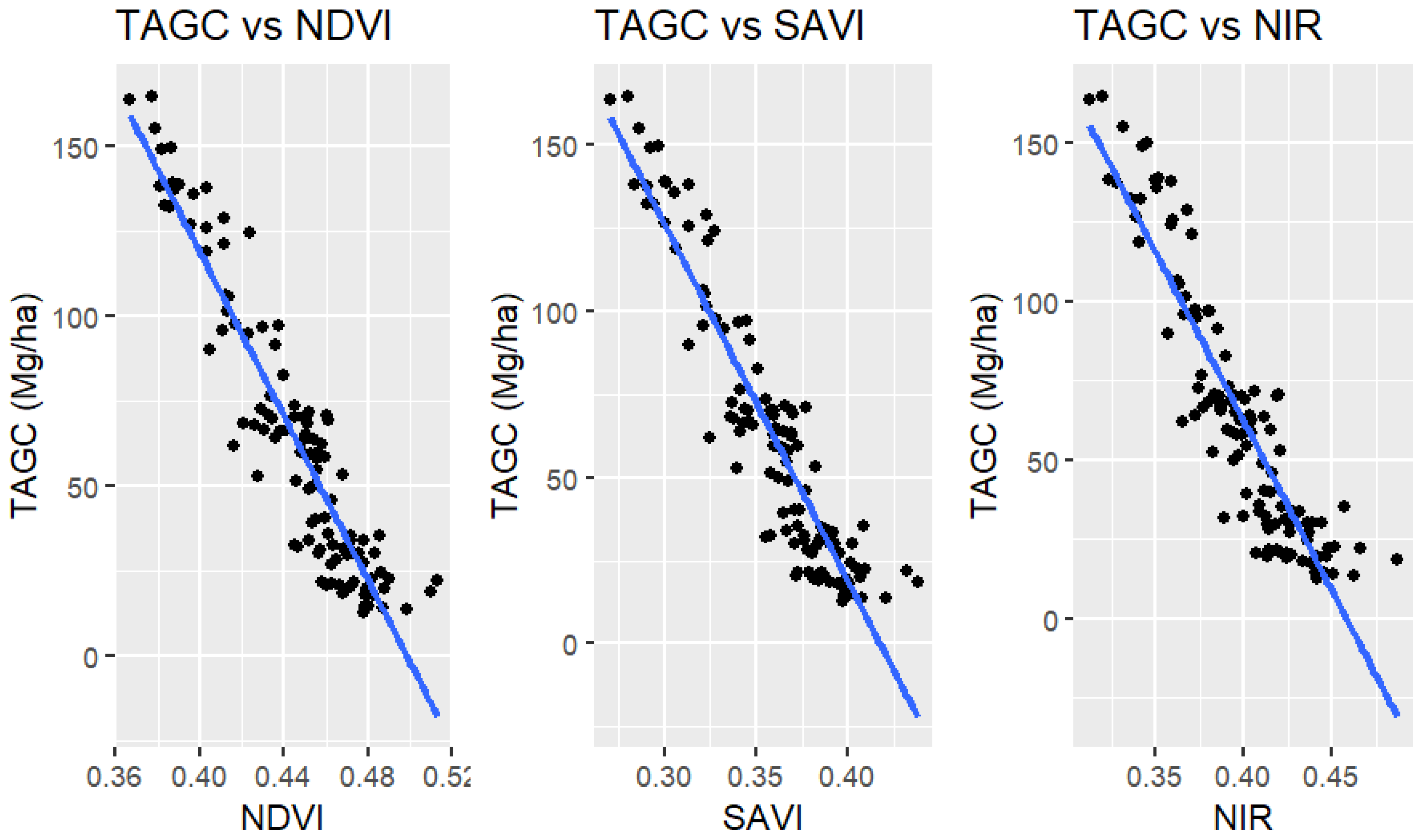
3.1. Vegetation Indices and Multispectral Bands Influencing Above-Ground Carbon

From the PCA results of 10 variables from the data of 115 sample plots (

Table 2. Result summary of PCA from 115 datasets of 10 variables.

	PC1	PC2	PC3	PC4	PC5	PC6	PC7	PC8	PC9	PC10
Standard deviation	2.8636	1.1976	0.4521	0.3336	0.2024	0.0923	0.0148	0.0051	0.0026	0.0011
Proportion of Variance	0.8200	0.1434	0.0204	0.0111	0.0041	0.0009	0.0000	0.0000	0.0000	0.0000
Cumulative Proportion	0.8200	0.9635	0.9839	0.9950	0.9991	1.0000	1.0000	1.0000	1.0000	1.0000

), the first two PCs were selected to analyze and determine the VIs and multispectral bands that have a large influence on TAGC to establish correlation models because these two PCs account for 96.35% of the variation of the original dataset.

Since PC1 accounts for the largest share of variance in the original dataset (82%), it was used to determine the weight of each of the 10 variables (

Table 3. Weight of variability by principal components.

Variable	PC1	PC2	PC3	PC4	PC5	PC6	PC7	PC8	PC9	PC10
TAGC	0.3243	−0.1708	0.0903	−0.9174	0.0501	−0.1154	0.0032	−0.0037	−0.0001	0.0007
NDVI	−0.3352	0.2288	−0.0572	−0.1489	−0.0633	−0.1696	−0.4412	−0.3152	−0.6856	0.1139
EVI	−0.3443	0.0762	−0.2778	−0.1636	−0.1221	−0.0163	0.5489	−0.6262	0.1721	−0.1829
SAVI	−0.3420	0.1606	−0.0066	−0.1760	−0.0599	0.1680	−0.1789	0.0147	0.4556	0.7447
ARVI	−0.3330	0.2355	−0.1884	−0.1869	−0.0615	0.0034	−0.4461	0.2438	0.3780	−0.5985
SIPI	−0.3270	0.1809	0.5963	−0.0173	−0.0553	−0.6063	0.2808	0.2305	0.0399	−0.0172
NIR	−0.3469	0.0510	0.0809	−0.2038	−0.0547	0.6048	0.3596	0.4413	−0.3643	−0.0580
RED	−0.2270	−0.6004	0.5318	0.0396	−0.2141	0.2608	−0.2507	−0.3108	0.0926	−0.1475
GREEN	−0.3204	−0.2941	−0.0743	−0.0082	0.8946	−0.0697	−0.0022	0.0016	0.0018	−0.0003
BLUE	−0.2335	−0.5909	−0.4748	0.0050	−0.3449	−0.3510	0.0455	0.3231	−0.0830	0.1240

) and to analyze the relationship matrix of these variables in the context of the correlation between PC1 and PC2 (Figure 3).

The equation indicating the weight of variables following PC1 is presented as follows:

PC1 = 0.3243373 × TAGC − 0.3351920 × NDVI − 0.3443245 × EVI − 0.3420016 × SAVI − 0.3329627 × ARVI − 0.3270426 × SIPI − 0.3469365 × NIR − 0.2269835 × RED − 0.3204391 × GREEN − 0.2335349 × BLUE

(7)

The variables BLUE, RED, and GREEN have small weights and are separate, with unclear effects on TAGC (Figure 3), so these variables are excluded from establishing correlation models. TAGC has a close and inverse relationship with the variables NDVI, EVI, SAVI, ARVI, SIPI, and NIR; these variables have a close relationship with each other in pairs, so they form variable groups in the regression model with TAGC, which are the groups (NDVI, ARVI), (SAVI, SIPI), and (NIR, EVI), respectively, represented in the yellow, red, and blue circles in Figure 3. In addition, in each of the above variable combinations, the variables NDVI, SAVI, and NIR have higher weights than the remaining variable (Table 3), so they are also selected to establish a regression model with TAGC in single-variable form.

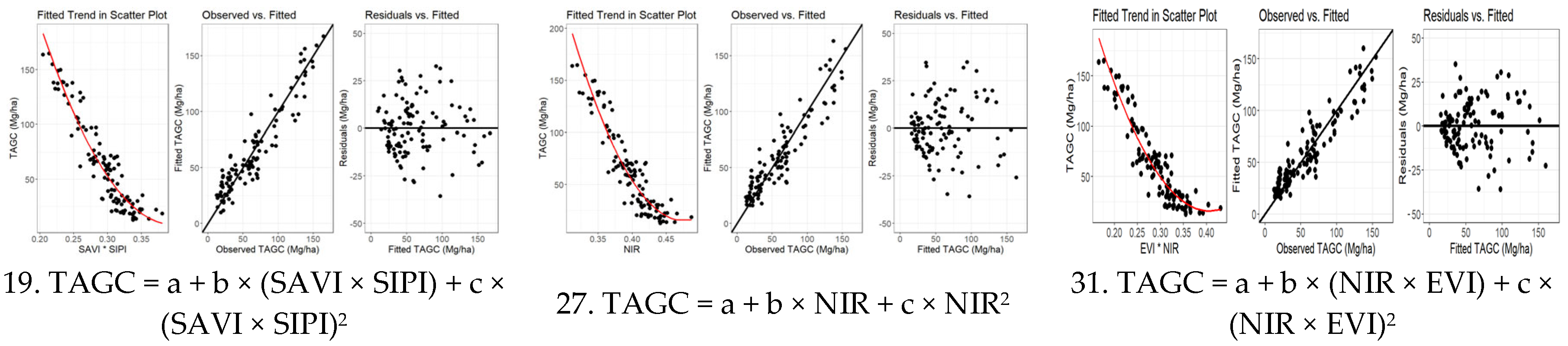
3.2. Establishment of Above-Ground Carbon Estimation Models

The PCA results selected three single variables and three variable combinations that have a significant influence on TAGC. An analysis of TAGC variations with respect to NDVI, SAVI, and NIR showed that TAGC differentiates strongly when these variables are small (Figure 4). Consequently, it is necessary to develop models of single variables or variable combinations with weight to improve the differentiation of the model’s predicted values (

Table 4. Established model forms with weights to select the optimal model.

Model	Correlation Equation Form	Weight
Linear	TAGC = f(NDVI)	1/NDVI−2
	TAGC = f(SAVI)	1/SAVI−2
	TAGC = f(NIR)	1/NIR−2
	TAGC = f(NDVI, ARVI)	1/NDVI−2
	TAGC = f(SAVI, SIPI)	1/SAVI−2
	TAGC = f(NIR, EVI)	1/NIR−2
Non-linear (Power, Exponential, Quadratic)	TAGC = f(NDVI)	1/NDVIδ
	TAGC = f(SAVI)	1/SAVIδ
	TAGC = f(NIR)	1/NIRδ
	TAGC = f(NDVI, ARVI)	1/NDVIδ
	TAGC = f(SAVI, SIPI)	1/SAVIδ
	TAGC = f(NIR, EVI)	1/NIRδ

).

From the equations presented in Table 4, 36 equations were established and compared for selecting fit models. The regression equations were established with an average AIC value of 766.691 (the smallest value was 748.717; the largest value was 785.717) and R² values ranging from 76.3% to 89.1%. Among these, 16 regression equations with an AIC < 766.691 (ranging from 748.983 to 765.790) and R² > 0.85 were chosen for estimating and testing the existence of parameters, including two linear equations of a single variable, one linear equation of variable combination, three non-linear equations of a single variable, and ten non-linear equations of variable combination (

Table 5. Result of model development with fit statistics.

ID	Equation Form	AIC	R2	ASE (%)	RMSE (Mg ha−1)	MPSE (%)
1	TAGC = a + b × NDVI	762.452	0.87215	0.75	15.08	34.47
2	TAGC = a × e(b × NDVI)	769.343	0.85502	−0.96	16.15	24.67
3	TAGC = a + b × NDVI + c × NDVI2	754.401	0.88567	4.76	14.34	33.30
4	TAGC = a × NDVIb	776.901	0.83989	−2.30	16.95	25.37
5	TAGC = a + b × (NDVI × ARVI)	773.041	0.85401	−8.30	16.32	35.60
6	TAGC = a × e(b × NDVI × ARVI)	762.113	0.87105	−3.02	15.28	23.96
7	TAGC = a + b × (NDVI × ARVI) + c × (NDVI × ARVI)2	752.085	0.88764	−59.26	14.36	90.02
8	TAGC = a × (NDVI × ARVI)b	774.778	0.84658	−2.11	16.70	25.88
9	TAGC = a + b × NDVI + c × ARVI	762.164	0.87367	−3.99	14.81	33.62
10	TAGC = a × e(b × NDVI + c × ARVI)	769.258	0.86312	−2.83	15.89	25.34
11	TAGC = a + b × NDVI + c × NDVI2 +d × ARVI + e × ARVI2	756.739	0.88757	1.76	14.19	32.49
12	TAGC = a × NDVIb × ARVIc	775.078	0.85231	−3.17	16.40	25.57
13	TAGC = a + b × SAVI	765.790	0.86697	−5.12	15.38	36.42
14	TAGC = a × e(b × SAVI)	762.800	0.85757	−2.84	16.35	23.62
15	TAGC = a + b × SAVI + c × SAVI2	748.983	0.88897	1.27	14.14	42.69
16	TAGC = a × SAVIb	772.618	0.82260	−1.70	17.68	24.74
17	TAGC = a + b × (SAVI × SIPI)	771.465	0.85792	−10.79	15.83	46.47
18	TAGC = a × e(b × SAVI × SIPI)	765.410	0.85607	−2.23	15.73	23.22
19	TAGC = a + b × (SAVI × SIPI) + c × (SAVI × SIPI)2	753.226	0.88436	4.28	13.88	26.51
20	TAGC = a × (SAVI × SIPI)^b	777.733	0.82186	−1.70	17.54	25.55
21	TAGC = a + b × SAVI + c × SIPI	766.979	0.86804	0.03	15.44	61.61
22	TAGC = a × e(b × SAVI + c × SIPI)	762.561	0.86136	−2.72	15.74	23.62
23	TAGC = a + b × SAVI + c × SAVI2 +d × SIPI + e × SIPI2	751.194	0.89076	3.02	14.39	29.86
24	TAGC = a × SAVIb × SIPIc	773.127	0.82525	−1.30	17.58	24.99
25	TAGC = a + b × NIR	785.321	0.83064	24.52	17.03	95.31
26	TAGC = a × e(b × NIR)	768.493	0.82896	−0.57	16.92	23.82
27	TAGC = a + b × NIR + c × NIR2	756.924	0.86649	0.70	15.50	23.17
28	TAGC = a × NIRb	775.476	0.78901	−0.84	18.75	24.77
29	TAGC = a + b × (NIR × EVI)	785.717	0.82968	−9.43	17.54	41.36
30	TAGC = a × e(b × NIR × EVI)	761.065	0.84910	−2.65	16.20	23.33
31	TAGC = a + b × (NIR × EVI) + c × (NIR × EVI)2	752.493	0.87647	−0.16	14.65	22.54
32	TAGC = a × (NIR × EVI)b	777.524	0.76316	−0.18	20.00	24.77
33	TAGC = a + b × NIR + c × EVI	776.007	0.85124	−7.96	15.90	51.13
34	TAGC = a × e(b × NIR + c × EVI)	768.716	0.82342	−0.27	17.77	24.71
35	TAGC = a + b × NIR + c × NIR2 +d × EVI + e × EVI2	756.972	0.87294	2.35	15.23	24.13
36	TAGC = a × NIRb × EVIc	775.920	0.78908	−0.02	19.85	25.11

Note: Bold: Selected models based on AIC and R² for estimating parameters.

).

3.3. Determination of Above-Ground Carbon Estimation Models

The fit models were estimated and tested for the existence of parameters with data from 115 samples (100% of the dataset). Among the 16 selected fit models, 9 models have parameters with a p-value < 0.001 and MPSE values ranging from 21.63% to 26.32% (lower than 30%), including 1 single-variable exponential model (Equation (14)), 2 exponential models of variable combination (Equations (6) and (18)), 3 single-variable quadratic models (Equations (3), (15), and (27)), and 3 quadratic models of variable combination (Equations (7), (19), and (31)) (

Table 6. Result of fit model selection with parameter estimation and fit statistics.

ID	Equation Form	Parameters		p-Value	Std. Error	R2	MPSE (%)
1	TAGC = a + b × NDVI	a	590	<0.001	20.8	0.87064	35.99
		b	−1181.4	<0.001	46.1
3	TAGC = a + b × NDVI + c × NDVI2	a	1523.206	<0.001	217.6896	0.88581	26.32
		b	−5441.707	<0.001	989.7512
		c	4837.304	<0.001	1121.616
6	TAGC = a × e(b × NDVI × ARVI)	a	2617.904	<0.001	356.5325	0.87025	23.62
		b	−26.8626	<0.001	1.0567
7	TAGC = a + b × (NDVI × ARVI) + c × (NDVI × ARVI)2	a	648.275	<0.001	53.1819	0.88712	23.03
		b	−6450.795	<0.001	743.7517
		c	16,281.53	<0.001	2576.696
9	TAGC = a + b × NDVI + c × ARVI	a	607.43	<0.001	22.71	0.87415	31.13
		b	−2406.51	<0.001	674.97
		c *	1644.34	0.071	903.84
11	TAGC = a + b × NDVI + c × NDVI2 +d × ARVI + e × ARVI2	a	1348.19	<0.001	256.874	0.88784	23.47
		b*	10,401.88	0.348	11,037.17
		c *	−12,747.94	0.291	12,032.41
		d *	−20,840.87	0.154	14,536.67
		e *	31,994.84	0.146	21,860.44
13	TAGC = a + b × SAVI	a	432.86	<0.001	15.47	0.86581	48.71
		b	−1031.04	<0.001	42.15
14	TAGC = a × e(b × SAVI)	a	14,563.32	<0.001	3089.371	0.85639	23.38
		b	−15.606	<0.001	0.6266
15	TAGC = a + b × SAVI + c × SAVI2	a	1070.272	<0.001	109.0798	0.88933	22.62
		b	−4640.056	<0.001	608.0028
		c	5060.527	<0.001	843.6183
18	TAGC = a × e(b × SAVI × SIPI)	a	4288.168	<0.001	701.5295	0.85790	23.42
		b	−14.784	<0.001	0.5977
19	TAGC = a + b × (SAVI × SIPI) + c × (SAVI × SIPI)2	a	754.192	<0.001	67.7088	0.88606	22.85
		b	−3758.794	<0.001	458.1902
		c	4737.115	<0.001	769.794
22	TAGC = a × e(b × SAVI + c × SIPI)	a *	387.9781	0.610	759.3648	0.86151	23.23
		b	−20.1558	<0.001	2.5505
		c *	6.3853	0.065	3.4379
23	TAGC = a + b × SAVI + c × SAVI2 +d × SIPI + e × SIPI2	a *	−762.477	0.795	2932.537	0.88978	22.24
		b	−5846.867	<0.001	1706.388
		c	6568.468	0.004	2266.891
		d *	4858.904	0.532	7756.204
		e *	−2845.5	0.543	4663.326
27	TAGC = a + b × NIR + c × NIR2	a	1537.576	<0.001	143.5515	0.86646	22.04
		b	−6398.241	<0.001	700.553
		c	6723.375	<0.001	852.3433
31	TAGC = a + b × (NIR × EVI) + c × (NIR × EVI)2	a	505.7588	<0.001	33.2636	0.87646	21.63
		b	−2411.523	<0.001	214.8227
		c	2967.038	<0.001	343.2117
35	TAGC = a + b × NIR + c × NIR2 +d × EVI + e × EVI2	a	1513.702	<0.001	205.311	0.87259	21.76
		b	−7727.276	0.018	3225.838
		c	8721.605	0.022	3780.838
		d *	790.201	0.563	1364.302
		e	−638.933	0.470	881.386

Note: Bold: Selected models based on cross-validation with MPSE < 30%; *: parameter with p-value > 0.05.

).

Among the nine models identified as fit models, the quadratic models showed the best AIC, R², and MPSE values. In particular, the variable combination model (NIR, EVI) (Equation (31)) and the single-variable NIR model (Equation (27)) had the best MPSE (lowest) and equivalent, at 21.63% and 22.04%, respectively (Table 6). In addition, these two models have fitted the trend in the middle of the data cloud (left) or closely follow the observed value on the diagonal (middle), and the residuals (right) have a narrow distribution and are all according to the fitted values (Figure 5). From these results, the two abovementioned models were determined to be optimal equations, in which one equation is representative of a single-variable quadratic model (TAGC = a + b × NIR + c × NIR²), and one is representative of a quadratic model with a variable combination (TAGC = a + b × (NIR × EVI) + c × (NIR × EVI)²).

4. Discussion

4.1. Determination of Indices of Sentinel-2 Imagery Influencing TAGC Prediction

Numerous studies have demonstrated the utility of satellite imagery for developing biomass estimation models through vegetation indices (VIs). However, the majority of these studies have focused on identifying correlations between Above-Ground Biomass (AGB) and individual VIs only [7,8,9,10,42,43]. Given that VIs are derived from multispectral bands—primarily BLUE, GREEN, RED, and near-infrared (NIR) [30]—there exists a more complex, multivariate relationship between Total Above-Ground Carbon (TAGC), VIs, and the underlying spectral bands. Therefore, it is essential to identify not only individual VIs but also combinations of VIs and spectral bands that are strongly associated with TAGC in order to construct robust regression models, whether in single-variable or variable combination forms.

Principal component analysis (PCA) results revealed that NDVI, SAVI, and the NIR band exert significant influence on TAGC. This finding aligns with that of Poudel et al. (2023), who reported that among 12 Sentinel-2-derived VIs, NDVI and SAVI exhibited the strongest relationships with AGB in both linear and quadratic models [43]. Unlike previous studies that typically relied on single indices to develop estimation models, this study further identified three combinations of variables—(NDVI, ARVI), (SAVI, SIPI), and (NIR, EVI)—that demonstrated strong correlations with TAGC. This multivariable approach helps preserve the richness of the original dataset. By applying PCA, the dimensionality of large datasets is reduced, interpretability is enhanced, and information loss is minimized [44].

Consistent with PCA results in previous studies—for example, the PCA of Dalat pine diameter growth and four ecological environmental factors (explaining 66.85% of variance) or nine climate factors (explaining 77.90%) [36]—this study adopted the common assumption that the first two principal components are sufficient if they account for at least 80% of the total variance. In this case, the cumulative variance of the first two components accounted for 96.35% of the total variability in the original dataset (Table 2), thus providing a strong basis for the reliable identification of VIs and multispectral bands associated with TAGC.

4.2. Establishment and Validation of Models for Predicting TAGC

Most publications related to the relationship model between AGB and Sentinel-2 image indices (ARVI, EVI, NDVI, SAVI, SIPI) are set up in a linear form without weight, so R² only reaches from 0.57 to 0.75 [43], the NDVI of the Landsat 8 image only gives R² = 0.43 [45], or the linearized log-log or log-lin function with EVI gives R² = 0.60–0.76 [8]. With the weighted linear equations between TAGC and single variables (NDVI, SAVI, NIR) or combinations of variables ((NDVI, ARVI), (SAVI, SIPI), or (NIR, EVI)) by the Ordinary Least Squares method in this study, R² = 0.83–0.87 (Table 5); this should be superior to the linear model or log-log, log-lin linearization. Similarly, with the weighted non-linear model established by the Maximum Likelihood method, R² = 0.76–0.89 (Table 5), which is also much higher than the research results of Poudel et al. (2023); R² = 0.72–0.78 with the quadratic form, R² = 0.55–0.61 with the power form, and R² = 0.53–0.62 with the exponential form [43]. This result has shown that establishing regression models, including both linear with weight and non-linear with weight models, improves error variability.

The quadratic, exponential, and power models all gave higher R² values than the linear model, respectively, as follows: R² = 0.87–0.89, R² = 0.82–0.87, and R² = 0.76–0.85 (Table 5). This result is similar to the study of Poudel et al. (2023); the quadratic models gave the highest R², followed by the exponential model and, finally, the power model [43]. Therefore, non-linear models should be established to increase reliability compared to the linear and linearized models because there is a complex, multivariate, and non-linear relationship between AGB/TAGC and VIs and multispectral bands.

Regarding model validation, most previous studies have not applied the cross-validation method but have mainly divided the dataset into two independent parts: 50% of the data was used to establish the model, and 50% of the data was for model validation [8,43,45]. This study applied the cross-validation method, with 80% of the data used to establish the model and 20% of the data for validation. The validation process was carried out with 100 iterations, so the models all had R² = 0.76–0.89 (Table 5), which was superior to previous studies, which all had R² < 0.78 [8,43,45].

5. Conclusions

Establishing TAGC estimation models based on VIs and multispectral bands of Sentinel-2 images plays an increasingly important role in estimating forest carbon stocks because this method increases reliability and reduces costs compared to the destructive method and can be applied at large scales, such as national, regional, and global. The NIR single-variable and combination of variables (NIR,EVI) non-linear models have been validated as appropriate, and they enhance the accuracy and applicability of the models for estimating TAGC in the South Central Coastal Ecoregion of Vietnam.

References

1. Huete, A.R. A soil-adjusted vegetation index (SAVI). Remote Sens. Environ. 1988, 25, 295–309. [Google Scholar] [CrossRef]
2. Gitelson, A.; Merzlyak, M.N. Remote estimation of chlorophyll content in higher plant leaves. Int. J. Remote Sens. 1997, 18, 2691–2697. [Google Scholar] [CrossRef]
3. Wu, J.; Chen, B.; Reynolds, G.; Xie, J.; Liang, S.; O’Brien, M.J.; Hector, A. Monitoring tropical forest degradation and restoration with satellite remote sensing: A test using Sabah Biodiversity Experiment. Adv. Ecol. Res. 2020, 62, 117–146. [Google Scholar] [CrossRef]
4. Tucker, C.J. Red and photographic infrared linear combinations for monitoring vegetation. Remote Sens. Environ. 1979, 8, 127–150. [Google Scholar] [CrossRef]
5. Baccini, A.; Friedl, M.A.; Woodcock, C.E.; Warbington, R. Forest biomass estimation over regional scales using multisource data. Geophys. Res. Lett. 2004, 31, 1–4. [Google Scholar] [CrossRef]
6. Pettorelli, N.; Vik, J.O.; Mysterud, A.; Gaillard, J.M.; Tucker, C.J.; Stenseth, N.C. Using the satellite-derived NDVI to assess ecological responses to environmental change. Trends Ecol. Evol. 2005, 20, 503–510. [Google Scholar] [CrossRef]
7. Priatama, A.R.; Setiawan, Y.; Mansur, I.; Masyhuri, M. Regression Models for Estimating Aboveground Biomass and Stand Volume Using Landsat-Based Indices in Post-Mining Area. J. Manaj. Hutan Trop. 2022, 28, 1–14. [Google Scholar] [CrossRef]
8. Dang, H.N.; Ba, D.D.; Trung, D.N.; Viet, H.N.H. A Novel Method for Estimating Biomass and Carbon Sequestration in Tropical Rainforest Areas Based on Remote Sensing Imagery: A Case Study in the Kon Ha Nung Plateau, Vietnam. Sustainability 2022, 14, 16857. [Google Scholar] [CrossRef]
9. Khan, K.; Iqbal, J.; Ali, A.; Khan, S.N. Assessment of Sentinel-2-Derived Vegetation Indices for the Estimation of Above-Ground Biomass/Carbon Stock, Temporal Deforestation, and Carbon Emissions Estimation in the Moist Temperate Forests of Pakistan. Appl. Ecol. Environ. Res. 2020, 18, 783–815. [Google Scholar] [CrossRef]
10. Askar, N.; Nuthammachot, N.; Phairuang, W.; Wicaksono, P.; Sayektiningsih, T. Estimating Aboveground Biomass on Private Forest Using Sentinel-2 Imagery. J. Sens. 2018, 2018, 6745629. [Google Scholar] [CrossRef]
11. Zhang, X.; Zhao, Y.; Ashton, M.S.; Lee, X. Measuring Carbon in Forests. In Managing Forest Carbon in a Changing Climate; Ashton, M., Tyrrell, M., Spalding, D., Gentry, B., Eds.; Springer: Dordrecht, The Netherlands, 2012. [Google Scholar] [CrossRef]
12. Naesset, E.; Gobakken, T.; Solberg, S.; Gregoire, T.G.; Ståhl, G.; Lange, H.; Dick, O.; Gobakken, T.; Astrup, R. Mapping and estimating forest area and aboveground biomass in miombo woodlands in Tanzania using data from airborne laser scanning, TanDEM-X, RapidEye, and global forest maps: A comparison of estimated precision. Remote Sens. Environ. 2016, 175, 282–300. [Google Scholar] [CrossRef]
13. McRoberts, R.E.; Næsset, E.; Gobakken, T. Estimation for inaccessible and non-sampled forest areas using model-based inference and remotely sensed auxiliary information. Remote Sens. Environ. 2014, 154, 226–233. [Google Scholar] [CrossRef]
14. Esteban, J.R.E.; Montealegre, A.L.; Miranda, D.; Segura, A.S.; Ruiz, M.M. A model-based volume estimator that accounts for both land cover misclassification and model prediction uncertainty. Remote Sens. 2020, 12, 3360. [Google Scholar] [CrossRef]
15. Jędrych, M.; Zagajewski, B.; Marcinkowska-Ochtyra, A. Application of Sentinel-2 and EnMAP new satellite data to the mapping of environmental changes. Pol. Cartogr. Rev. 2017, 49, 107–119. [Google Scholar] [CrossRef]
16. Nguyen, T.D.; Kappas, M. Estimating forest aboveground biomass (AGB) by integrating SPOT-6 data with field-based measurements using the random forest (RF) algorithm. J. Sens. 2020, 4216160. [Google Scholar] [CrossRef]
17. Moradi, F.; Darvishsefat, A.A.; Pourrahmati, M.R.; Deljouei, A.; Borz, S.A. Estimating aboveground biomass in dense Hyrcanian forests by the use of Sentinel-2 data. Forests 2022, 13, 104. [Google Scholar] [CrossRef]
18. Ma, T.; Hu, Y.; Wang, J.; Beckline, M.; Pang, D.; Chen, L.; Ni, X.; Li, X. A novel vegetation index approach using Sentinel-2 data and Random Forest algorithm for estimating forest stock volume in the Helan Mountains, Ningxia, China. Remote Sens. 2023, 15, 1853. [Google Scholar] [CrossRef]
19. Huy, B.; Truong, N.Q.; Poudel, K.P.; Temesgen, H.; Khiem, N.Q. Multi-output deep learning models for enhanced reliability of simultaneous tree above- and below-ground biomass predictions in tropical forests of Vietnam. Comput. Electron. Agric. 2024, 204, 109080. [Google Scholar] [CrossRef]
20. Cheng, F.; Ou, G.; Wang, M.; Liu, C. Remote sensing estimation of forest carbon stock based on machine learning algorithms. Forests 2024, 15, 681. [Google Scholar] [CrossRef]
21. Phuong, V.T.; Inoguchi, A.; Birigazzi, L.; Henry, M.; Sola, G. Introduction and Background of the Study. In Tree Allometric Equation Development for Estimation of Forest Above-Ground Biomass in Viet Nam (Part A); Inoguchi, A., Henry, M., Birigazzi, L., Sola, G., Eds.; UN-REDD Programme: Hanoi, Vietnam, 2012. [Google Scholar]
22. Huy, B. Allometric Model and Remote Sensing-GIS to Estimate Carbon Removal of Evergreen Broadleaf Forests in the Central Highland Region; Publication House of Science and Technique: Hanoi, Vietnam, 2013. [Google Scholar]
23. Phuong, V.T.; Linh, N.T.M. Final Report on Forest Ecological Stratification in Vietnam; UN-REDD Programme: Hanoi, Vietnam, 2011. [Google Scholar]
24. Sola, G.; Inoguchi, A.; Garcia-Perez, J.; Donegan, E.; Birigazzi, L.; Henry, M. Allometric Equations at National Scale for Tree Biomass Assessment in Viet Nam: Context, Methodology and Summary of the Results; UN-REDD Programme: Hanoi, Vietnam, 2014. [Google Scholar]
25. Da Nang Portal. Location and Natural Conditions. Available online: https://danang.gov.vn/web/en/detail?id=26029&_c=16407111 (accessed on 19 March 2025).
26. Ministry of Agriculture and Rural Development. Decision 816/QD-BNN-KL on National Forest Status Announcement in 2023; 20 March 2024. Available online: https://thuvienphapluat.vn/van-ban/Tai-nguyen-Moi-truong/Quyet-dinh-816-QD-BNN-KL-2024-cong-bo-hien-trang-rung-toan-quoc-604807.aspx (accessed on 3 April 2025).
27. Ministry of Agriculture and Rural Development. Circular No. 33/2018/TT-BNNPTNT on Prescribing Forest Survey, Inventory and Forest Transition Monitoring; 16 November 2018. Available online: https://lawnet.vn/en/vb/Circular-33-2018-TT-BNNPTNT-prescribing-forest-survey-inventory-forest-transition-monitoring-67B66.html (accessed on 19 March 2025).
28. Huy, B.; Poudel, K.P.; Temesgen, H. Aboveground biomass equations for evergreen broadleaf forests in South Central Coastal ecoregion of Viet Nam: Selection of eco-regional or pantropical models. For. Ecol. Manag. 2016, 376, 276–283. [Google Scholar] [CrossRef]
29. IPCC. Guidelines for National Greenhouse Gas Inventories; Eggleston, H.S., Buendia, L., Miwa, K., Ngara, T., Tanabe, K., Eds.; IGES: Hayama, Japan, 2006. [Google Scholar]
30. Xue, J.; Su, B. Significant Remote Sensing Vegetation Indices: A Review of Developments and Applications. J. Sens. 2017, 2017, 1353691. [Google Scholar] [CrossRef]
31. Kaufman, Y.J.; Tanre, D. Atmospherically Resistant Vegetation Index (ARVI) for EOS-MODIS. IEEE Trans. Geosci. Remote Sens. 1992, 30, 261–270. [Google Scholar] [CrossRef]
32. Huete, A.; Didan, K.; Miura, T.; Rodriguez, E.P.; Gao, X.; Ferreira, L.G. Overview of the Radiometric and Biophysical Performance of the MODIS Vegetation Indices. Remote Sens. Environ. 2002, 83, 195–213. [Google Scholar] [CrossRef]
33. Peñuelas, J.; Filella, I.; Lloret, P.; Muñoz, F.; Vilajeliu, M. Reflectance Assessment of Mite Effects on Apple Trees. Int. J. Remote Sens. 1995, 16, 2727–2733. [Google Scholar] [CrossRef]
34. R Core Team. A Language and Environment for Statistical Computing; R Foundation for Statistical Computing: Vienna, Austria, 2023; Available online: http://www.r-project.org/index.html (accessed on 13 October 2024).
35. Greenacre, M.; Groenen, P.J.; Hastie, T.; d’Enza, A.I.; Markos, A.; Tuzhilina, E. Principal Component Analysis. Nat. Rev. Methods Primers 2022, 2, 100. [Google Scholar] [CrossRef]
36. Huy, B.; Nam, L.C.; Poudel, K.P.; Temesgen, H. Individual Tree Diameter Growth Modeling System for Dalat Pine (Pinus dalatensis Ferré) of the Upland Mixed Tropical Forests. For. Ecol. Manag. 2021, 480, 118612. [Google Scholar] [CrossRef]
37. Huy, B.; Truong, N.Q.; Khiem, N.Q.; Poudel, K.P.; Temesgen, H. Stand Growth Modeling System for Planted Teak (Tectona grandis L.f.) in Tropical Highlands. Trees People 2022, 9, 100308. [Google Scholar] [CrossRef]
38. Picard, N.; Saint-André, L.; Henry, M. Manual for Building Tree Volume and Biomass Allometric Equations: From Field Measurement to Prediction; FAO: Italy, Rome; Centre de Coopération Internationale en Recherche Agronomique pour le Développement: Montpellier, France, 2012; 215p.
39. Huy, B.; Khiem, N.Q.; Truong, N.Q.; Poudel, K.P.; Temesgen, H. Additive Modeling Systems to Simultaneously Predict Aboveground Biomass and Carbon for Litsea glutinosa of Agroforestry Model in Tropical Highlands. For. Syst. 2023, 32, e006. [Google Scholar] [CrossRef]
40. Akaike, H. Information Theory and an Extension of the Maximum Likelihood Principle. In Proceedings of the 2nd International Symposium on Information Theory; Akademiai Kiado: Budapest, Hungary, 1973; pp. 267–281. [Google Scholar]
41. Zeng, W.; Zhang, L.; Chen, X.; Cheng, Z.; Ma, K.; Li, Z. Construction of Compatible and Additive Individual-Tree Biomass Models for Pinus tabulaeformis in China. Can. J. For. Res. 2017, 47, 467–475. [Google Scholar] [CrossRef]
42. Pandit, S.; Tsuyuki, S.; Dube, T. Estimating Above-Ground Biomass in Sub-Tropical Buffer Zone Community Forests, Nepal, Using Sentinel-2 Data. Remote Sens. 2018, 10, 601. [Google Scholar] [CrossRef]
43. Poudel, A.; Shrestha, H.L.; Mahat, N.; Sharma, G.; Aryal, S.; Kalakheti, R.; Lamsal, B. Modeling and Mapping of Aboveground Biomass and Carbon Stock Using Sentinel-2 Imagery in Chure Region, Nepal. Int. J. For. Res. 2023, 2023, 5553957. [Google Scholar] [CrossRef]
44. Jolliffe, I.T.; Cadima, J. Principal Component Analysis: A Review and Recent Developments. Philos. Trans. R. Soc. A 2016, 374, 20150202. [Google Scholar] [CrossRef] [PubMed]
45. Luong, V.N.; Tateishi, R.; Kondoh, A.; Sharma, R.C.; Hoan, T.N.; Tu, T.T.; Minh, D.H.T. Mapping Tropical Forest Biomass by Combining ALOS-2, Landsat 8, and Field Plots Data. Land 2016, 5, 31. [Google Scholar] [CrossRef]
Figure 1. Location https://www.worldagroforestry.org/output/wood-density-database accessed on 13 October 2023).
Forests 16 00686 g001
Figure 2. Location of sample plots representing forest classes in the study area.
Forests 16 00686 g002
Figure 3. Biplot of variable weights of principal component 1 versus principal component 2.
Forests 16 00686 g003
Figure 4. TAGC volatility by NDVI, SAVI, and NIR.
Forests 16 00686 g004
Figure 5. Comparison of fitted trend in scatter plot, observed vs. fitted, and residuals vs. fitted (left to right) of 9 selected equations.
Forests 16 00686 g005aForests 16 00686 g005b