Tackling the Wildfire Prediction Challenge: An Explainable Artificial Intelligence (XAI) Model Combining Extreme Gradient Boosting (XGBoost) with SHapley Additive exPlanations (SHAP) for Enhanced Interpretability and Accuracy

Abstract

The intensification of global climate change, combined with increasing human activities, has significantly increased wildfire frequency and severity, posing a major global environmental challenge. As an illustration, Guizhou Province in China encountered a total of 221 wildfires over a span of 12 days. Despite significant advancements in wildfire prediction models, challenges related to data imbalance and model interpretability persist, undermining their overall reliability. In response to these challenges, this study proposes an explainable wildfire risk prediction model (EWXS) leveraging Extreme Gradient Boosting (XGBoost), with a focus on Guizhou Province. The methodology involved converting raster and vector data into structured tabular formats, merging, normalizing, and encoding them using the Weight of Evidence (WOE) technique to enhance feature representation. Subsequently, the cleaned data were balanced to establish a robust foundation for the EWXS model. The performance of the EWXS model was evaluated in comparison to established models, such as CatBoost, using a range of performance metrics. The results indicated that the EWXS model achieved an accuracy of 99.22%, precision of 98.48%, recall of 96.82%, an F1 score of 97.64%, and an AUC of 0.983, thereby demonstrating its strong performance. Moreover, the SHAP framework was employed to enhance model interpretability, unveiling key factors influencing wildfire risk, including proximity to villages, meteorological conditions, air humidity, and variations in vegetation temperature. This analysis provides valuable support for decision-making bodies by offering clear, explanatory insights into the factors contributing to wildfire risk.

1. Introduction

Wildfires, as highly destructive natural events, not only have severe impacts on ecological systems, but also result in significant socio-economic repercussions [1]. With the intensification of global climate change and the expansion of human activities, the frequency and intensity of wildfires have notably increased worldwide [2]. The year 2025 exemplified this trend with catastrophic events, such as the California wildfires. In January 2025, two major fires—“Eaton” and “Palisades”—devastated Los Angeles, burning over 152 square kilometers (57 km² and 95 km², respectively), destroying 16,000 structures, and causing economic losses estimated at USD 250–275 billion, making them the costliest natural disasters in US history. These fires claimed 29 lives and displaced 180,000 residents, highlighting systemic challenges, including inadequate firefighting infrastructure and delayed emergency responses. According to the latest data from the National Forestry Fire Prevention and Extinguishment Department, Guizhou Province, China, faced 221 wildfires within just 12 days, which attracted significant attention. The prevention of wildfires is crucial for protecting natural life and ensuring a healthy world for future generations [3]. Furthermore, wildfires not only cause ecological destruction, socio-economic losses, and fatalities, but also strain resource allocation efforts, presenting significant challenges in emergency response and recovery.

Traditionally, wildfire monitoring and prediction have primarily relied on ground patrols, satellite remote sensing technologies, and basic meteorological indicators. While these conventional methods have contributed to early detection and the issuance of warnings, their limitations have become increasingly evident in the context of complex environmental changes and dynamic wildfire patterns. Specifically, ground patrols are constrained by both manpower and geographic limitations, while satellite remote sensing technologies, despite their capacity for extensive area coverage, are limited by resolution in capturing intricate and variable factors. As a result, traditional monitoring and prediction methods do not fully meet current demands.

The rapid advancement of artificial intelligence and data science has prompted researchers to increasingly apply machine learning techniques to wildfire prediction studies. These studies primarily focus on two key areas: the prediction of wildfire risk and the forecasting of areas impacted by wildfires. For example, the studies cited in this context include various models used for risk prediction, such as the Artificial Neural Network [4], Enhanced Regression Tree [5], Backpropagation Neural Network [6], Convolutional Neural Network [7], Gradient Boosting Decision Tree [8], Support Vector Machine [9], Random Forest [10], Multilayer Perceptron [11], XGBoost [12], AdaBoost [13], and Deep Learning Model [14]. In contrast, studies [15,16,17,18,19,20,21] employed models that incorporate deep learning, fuzzy neural networks, artificial neural networks, and random forests to forecast wildfire-affected areas. Although neural networks and ensemble tree models exhibit strong predictive capabilities, they generally lack the necessary interpretability, which is crucial for practical wildfire prediction applications. Adequate model interpretability allows managers to not only better understand and assess the factors contributing to wildfire occurrences, but also helps the public to comprehend the rationale behind government decisions. This, in turn, promotes greater public cooperation with emergency response efforts, which can significantly reduce casualties. Furthermore, by providing clear explanations, areas at higher risk for wildfires can be identified, enabling authorities to allocate resources more effectively and proactively. This targeted approach ensures that the most vulnerable regions receive the necessary attention and resources to prevent or mitigate potential fire hazards. To address the performance limitations of current wildfire risk prediction models and the interpretability challenges in existing methodologies, this paper proposes an explainable wildfire prediction model based on Extreme Gradient Boosting, termed EWXS (Explaining Wildfire with XGBoost and SHAP). This study addresses the following three aspects:

• Data Collection and Feature Engineering: Initially, ArcGIS10.8 software was used to process orbital level imagery and vector data, which were geographically registered to fire point locations and converted into structured tabular data. These data were then combined with meteorological information to construct a comprehensive dataset. Feature engineering techniques, such as Weight of Evidence (WOE) encoding, were applied to enhance feature representation [22]. Additionally, to address the data imbalance, Random Over Sampling was employed, providing a solid foundation for model development and analysis.
• Model Construction: Using the dataset derived from the feature engineering process, EWXS constructs a wildfire prediction model based on the XGBoost algorithm. The model is evaluated using key performance metrics, including accuracy, recall, specificity, F1 score, and AUC. It is also compared with models from the existing literature to assess the comparative efficacy of EWXS.
• Enhancing Model Interpretability: Given the proven efficacy of Particle Swarm Optimization (PSO) in high-dimensional hyperparameter spaces [23], the hyperparameters of EWXS were optimized through 500 swarm iterations. Additionally, the SHAP framework was employed to conduct a detailed analysis of the features influencing wildfires. The study identified proximity to villages, meteorological conditions, air humidity, and temperature differentials as key factors influencing wildfire occurrences, aligning with the findings of Nur et al. [9] and Abdollahi et al. [24]. Specifically, the fire risk was found to be highest within a 0–2.7 km radius from villages, decreasing progressively with increasing distance and stabilizing beyond 8.07 km.

2. Related Research

Accurate wildfire prediction is crucial for environmental conservation, maintaining ecological balance, and ensuring human safety. Effective wildfire prediction not only mitigates fire-related damage, but also improves resource allocation and optimizes disaster response strategies. With the rapid advancement of artificial intelligence and data science, the application of these technologies in wildfire prediction has increased, offering innovative solutions for fire prevention [25]. The following provides a comprehensive analysis and synthesis of key aspects, including datasets used, research domains, methods for addressing data imbalance, model performance, and interpretability in the existing literature, highlighting current trends in the field.

In research on wildfires in China, Zhang H et al. [5] developed a wildfire prediction model for Inner Mongolia using an Enhanced Regression Tree, achieving an accuracy of 89.3% and an AUC (Area Under the Curve) value of 0.93. Zhang J et al. [7] integrated MCD64A1 monthly fire point data, terrain data, and climate data with Convolutional Neural Networks (CNNs) to develop a wildfire prediction model, achieving over 90% in all performance metrics. Xi J et al. [8] proposed a Gradient Boosting Decision Tree (GBDT)-based prediction model for the Jialing River Basin in Chongqing, achieving an accuracy of 95% and an AUC value of 0.983. Cao L et al. [10] used wildfire and meteorological data from Yantian, Jilin (2000–2019) to construct a Random Forest prediction model, achieving an accuracy of 93.8%.

In the international research domain, Nur A S et al. [9] applied an enhanced Support Vector Machine (SVM) to model wildfire data from Sydney, Australia, achieving an AUC value of 0.882 and an RMSE of 0.006. Pérez-Porras FJ et al. [11] pioneered the use of SMOTE (Synthetic Minority Over Sampling Technique) and SMOTETK (SMOTE + Tomek Links) techniques for oversampling MODIS data from Spain and employed a Multilayer Perceptron (MLP) for wildfire risk prediction, achieving a recall of 75% and an F1 score of 60%. Xu S et al. [6] and Dong H et al. [12] independently developed wildfire prediction models using the wildfire dataset from the UCI Machine Learning Repository. Notably, the XGBoost-based model presented by Dong H et al. [12] demonstrated superior performance compared to other approaches. Rubi J N S et al. [13] constructed a predictive model based on AdaBoost and Brazilian wildfire data, attaining an AUC value of 0.993. Tavakkoli Piralilou S et al. [14] also used Random Forest to model wildfire data from Gillan, Iran, attaining an accuracy of 92.5% and an AUC value of 0.947. Abdollahi A et al. [24] developed a deep learning model for wildfire risk prediction in Victoria, Australia, achieving an accuracy of 93% and an AUC value of 0.91. Qiu L et al. [26] used Random Forest for wildfire risk prediction in California, achieving an AUC value of 0.98 and a Kappa value of 0.92.

As illustrated in

Table 1. Comprehensive comparison of existing literature.

Author	Dataset	Country/Region	Methods for Addressing Data Imbalance	Model	Performance Outcomes	Interpretability	Explanation of the Sample Decision-Making Process
Zhang H et al. [5]	Historical wildfire data from Inner Mongolia covering the period from 1981 to 2020	Inner Mongolia, People’s Republic of China	None	Enhanced Regression Tree	Accuracy: 89.3% AUC: 93%	None	None
Xu S et al. [6]	UCI public wildfire dataset, encompassing data from Montesano National Park in Algeria and Northern Portugal	Algeria and Northern Portugal	None	BPNN	Accuracy: 78.89% Precision: 78.68% Recall: 54.33% AUC: 79.31%	None	None
Zhang J et al. [7]	MCD64A1 monthly fire product data in conjunction with terrain and climate datasets	Ding-a-ling Region, Inner Mongolia, People’s Republic of China	None	Convolutional Neural Network	Accuracy: 95% Precision: >90% Recall: >90% AUC: 83.8%	None	None
Xi J et al. [8]	Fire point data from the Jialing River Basin in Chongqing, spanning from 2018 to 2022	Chongqing, People’s Republic of China	None	GBDT	Accuracy: 95% AUC: 0.983	None	None
Nur A. S. et al. [9]	VIIRS-Suomi thermal anomaly fire data from Sydney, covering the period from 2011 to 2020	Sydney, New South Wales, Australia	None	SVR-PSO	AUC: 88.2% RMSE: 0.006	None	None
Cao L et al. [10]	Wildfire and meteorological data from Yantian, Jilin, covering the period from 2000 to 2019	Yantian Korean Autonomous Prefecture, Jilin Province, People’s Republic of China	None	Random Forest	Accuracy: 93.80%	None	None
Pérez-Porras FJ et al. [11]	Data derived from Landsat and MODIS imagery in Southern Spain	Huelva Province, located in Western Andalusia, Spain	SMOTE and SMOTETK	MLP	Recall: 75% F1: 60%	None	None
Dong H et al. [12]	Historical wildfire data from Montesano Natural Park in Portugal, available in the UCI Machine Learning Repository	Portugal	None	XGB	Accuracy: 81.32% F1: 78.62% AUC: 80.5%	None	None
Rubi J N S et al. [13]	Satellite and climate data collected over the past 20 years	Brazil	None	AdaBoost	AUC: 99.3%	Feature importance analysis method	None
Tavakkoli Piralilou S et al. [14]	MODIS thermal anomaly products combined with GPS-based wildfire location data	Gillan Province, Iran	None	Random Forest	Accuracy: 92.5% AUC: 0.947	None	None
Abdollahi A et al. [24]	MODIS fire point data, historical records, Sentinel-2 imagery, and additional meteorological datasets	Victoria, Australia	None	Deep Learning Model	Accuracy: 93% AUC: 0.91	Feature importance analysis method	Yes
Qiu L et al. [26]	Data on wildfire events and burnt areas from California, spanning from 1981 to 2019	California, United States of America	None	Random Forest	AUC: 98% Kappa: 0.92	SHapley values method	Yes

, despite significant progress in wildfire prediction performance using ensemble models such as Random Forest, Enhanced Regression Tree, and AdaBoost, as well as neural network models, notable shortcomings remain in handling data imbalance and enhancing model interpretability.

• Handling of Imbalanced Data: Wildfire datasets often exhibit significant class imbalance, as fire incidents are relatively rare compared to non-fire events. This imbalance can lead to models that are biased towards predicting non-fire cases, as they optimize for overall accuracy rather than correctly identifying minority class events. Consequently, models may struggle to detect actual wildfire risks, reducing their practical applicability in fire prevention and emergency response. To mitigate this issue, various resampling techniques, cost-sensitive learning approaches, and anomaly detection methods have been proposed, yet many studies still fail to effectively address the problem.
• Model Interpretability: While ensemble learning models and deep neural networks have significantly improved prediction accuracy, they often function as black boxes, offering limited insight into their decision-making processes. In wildfire risk prediction, model interpretability is crucial not only for scientific transparency, but also for practical implementation. Decision-makers, including government agencies and emergency responders, require clear explanations of predictive outcomes to develop effective mitigation strategies. Traditional explainability techniques such as feature importance ranking and partial dependence plots provide some insights, but they fail to capture complex feature interactions inherent in wildfire prediction. Therefore, enhancing model interpretability remains an urgent research challenge.

To address the identified deficiencies in handling data imbalance and model interpretability in existing research, this paper introduces the EWXS model. First, a multi-source heterogeneous dataset was constructed. To counteract class imbalance, the Random Over Sampling technique was applied to generate synthetic wildfire instances, ensuring a more balanced distribution between fire and non-fire cases. This approach improves the model’s ability to recognize minority class patterns, thereby enhancing prediction performance and generalizability. Additionally, the SHAP framework was employed to analyze key factors influencing wildfire occurrence, offering a deeper understanding of feature dependencies and decision-making processes.

3. Research Area and Data Construction

3.1. Introduction to the Research Area

Guizhou Province is located on the Yunnan-Guizhou Plateau in Southwestern China, with geographic coordinates ranging from 103°36′ to 109°35′ east longitude and 24°37′ to 29°13′ north latitude. This region serves as the watershed divide between the Yangtze and Pearl River systems and lies within the subtropical monsoon climate zone. The climate is characterized by mild winters, cool summers, concentrated rainfall, and relatively short durations of sunlight. The average annual temperature ranges from 12 °C to 19 °C, while annual precipitation fluctuates between 1100 mm and 1300 mm [27].

These climatic conditions support a wide variety of plant species. Common tree species include spruce, red pine, white birch, Amur linden, larch, and Mongolian oak [10]. Many of these species, such as red pine and larch, have high resin content and are highly flammable, making them particularly susceptible to ignition and rapid fire spread, especially during dry seasons. Additionally, the accumulation of leaf litter and organic debris in forested areas serves as fuel, further increasing wildfire risk. As shown in Figure 1, Guizhou’s complex topography, characterized by steep slopes and deep valleys, can influence wildfire behavior by facilitating rapid fire spread on sloped terrain, which complicates fire suppression efforts in mountainous regions.

3.2. Data Sources

The data used in this study were obtained from authoritative institutions and publicly available platforms, ensuring both accuracy and reliability. The dataset encompasses various dimensions, including fire point data, geographic factors, meteorological variables, and human activity indicators, enabling a comprehensive analysis. Detailed information on the data sources is provided in

Table 2. Detailed information on data sources.

Influencing Factors		Data Type	Data Source	Source Website
Geographic Factors	Elevation	Continuous	Geospatial Data Cloud Platform	https://www.gscloud.cn/search (accessed on 4 May 2024)
	NDVI	Continuous
	Slope Gradient	Continuous
	Slope Position	Discrete
	Slope Aspect	Continuous
	Monthly Vegetation Coverage Data	Discrete	National Tibetan Plateau Science Data Center	https://data.tpdc.ac.cn/zh-hans/data/f3bae344-9d4b-4df6-82a0-81499c0f90f7 (accessed on 4 May 2024)
	Soil Moisture	Continuous
	Land Cover Data	Discrete	Global Land Cover Data	https://www.gscloud.cn/ (accessed on 4 May 2024)
Meteorological Factors	Maximum Temperature	Continuous	2345 Historical Weather Data CnopenData Database	https://tianqi.2345.com/ (accessed on 4 May 2024) https://www.cnopendata.com/ (accessed on 4 May 2024)
	Minimum Temperature	Continuous
	Wind Speed	Continuous
	Wind Direction	Discrete
	Weather	Discrete
	Humidity	Continuous
Human Activity Factors	Distance to Railway	Continuous	OpenStreetMap	https://www.openstreetmap.org/ (accessed on 4 May 2024)
	Distance to River	Continuous
	Distance to Major Road	Continuous
	Distance to Major Settlement	Continuous
	Number of Villages within a 5 km Radius	Continuous
Other Factors	County Affiliation	Discrete	CnopenData Database
	GDP Grid Data	Continuous	Cubic Database	https://www.cnopendata.com/ (accessed on 4 May 2024)
	Electricity Consumption Grid Data	Continuous
Fire Point Data		Discrete	Institute of Remote Sensing and Digital Earth, Chinese Academy of Sciences	http://satsee.radi.ac.cn:8080/index.html (accessed on on 4 May 2024)

.

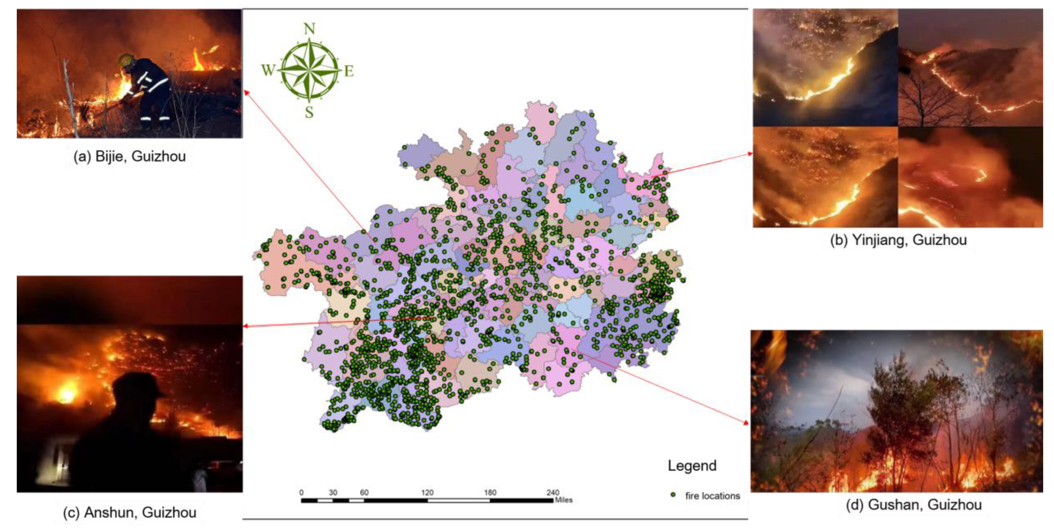
• Fire Point Data: The fire point data used in this study were derived from satellite hotspot data provided by the Institute of Remote Sensing and Digital Earth, Chinese Academy of Sciences [28]. This dataset spans from 2013 to 2021 and includes 16,331 samples, comprising 2721 fire points and 13,610 non-fire points. It provides essential information on the spatial distribution of wildfires, with fire point samples shown in Figure 2.

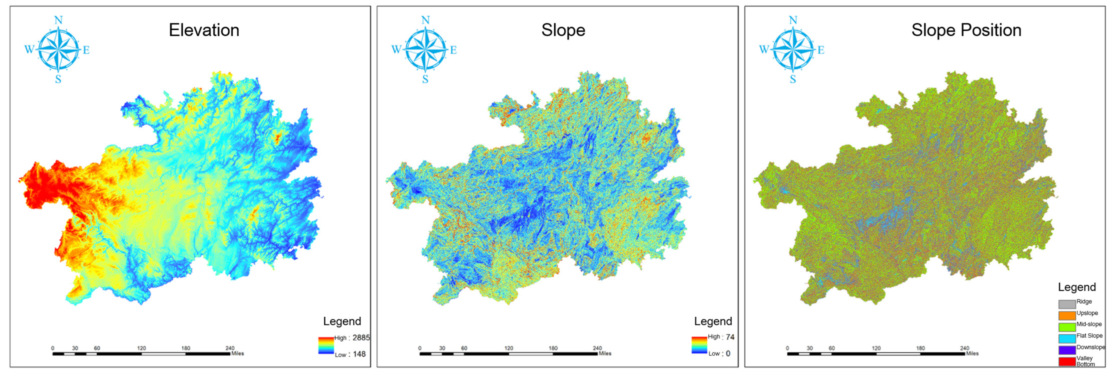
• Geographic Factor Data: Data on the 90 m resolution Digital Elevation Model (DEM), slope, aspect, and location were obtained from the Geospatial Data Cloud platform. Monthly vegetation coverage and soil moisture data were sourced from the National Tibetan Plateau Data Center, facilitating the assessment of vegetation conditions and soil moisture on wildfire occurrences. Land cover data, provided by GlobalLand30, include crucial surface characteristic information and are accessible through the Global Land Cover Data website.
• Meteorological Factor Data: Meteorological data, including temperature, humidity, and wind speed, were sourced from the CnopenData database and the 2345 Weather website.
• Human Activity Factor Data: Vector data were obtained from OpenStreetMap, and grid data were sourced from the Cubic Database. This includes distances to railways, rivers, major roads, and significant settlements, as well as the number of villages within a 5 km radius.

3.3. Data Construction

3.3.1. Data Spatialization and Integration

This section describes the process of constructing a spatial dataset from raw data through standardized procedures to enhance the model’s accuracy in identifying and predicting wildfire events. These procedures are essential for ensuring the precision and applicability of the analysis results, forming the foundation for capturing and analyzing key spatial factors influencing wildfire risk. The primary steps include:

• Buffer Zone Establishment and Sample Point Generation: A 500 m buffer radius around fire ignition points was selected based on previous studies demonstrating that this scale effectively captures fuel continuity and initial spread patterns in grassland-forest ecotones [29]. Non-fire points were then randomly generated outside this buffer zone at a 1:5 ratio. This ratio has been widely adopted in similar studies [30]. This fire-to-non-fire ratio balances the dataset, mitigates bias toward fire occurrences, and enhances model generalizability by adequately representing both fire and non-fire conditions.
• Raster Data Transformation: Spatial mapping of raster data was conducted using ArcMap10.8 software. The georeferencing process employed the WGS 84 (World Geodetic System 1984) coordinate system, a globally accepted standard for precise spatial referencing. The data were aligned with known geographic features to ensure spatial accuracy, and quality control checks were implemented to verify the precision of the georeferenced data. Additionally, the “Extract Values to Points” tool was used to extract key information from geographic and raster datasets, ensuring consistency across the dataset.
• Vector Data Transformation: As shown in Figure 3, for vector data, such as railways and rivers, nearest neighbor analysis tools were applied to calculate the shortest distance from sample points to these features. A 5 km buffer zone centered on villages was established, and the number of villages within this zone was quantified to assess their potential impact on wildfire occurrences.

• Data Integration: The structured data were consolidated and exported through table conversion tools. Meteorological data were then integrated to create a comprehensive dataset encompassing meteorological factors.

3.3.2. Construction of Derived Variables

Given the diverse factors influencing wildfire occurrences, this study derives a series of variables from existing data to enhance the understanding of fire risk factors.

• Meteorological Factor-Derived Variables: In addition to maximum and minimum temperatures, this study incorporates temperature differences, average temperatures, and the average maximum and minimum temperatures from the previous month. Weather-related variables are derived from the number of rainy and sunny days and include categorical weather conditions such as sunny, cloudy, overcast, rainy, or snowy.
• Human Factor-Derived Variables: This study calculates the average number of fire days per month for each county, as well as the average distances to railways and highways. In addition, it considers various ethnic festivals in Guizhou Province, including the Miao ethnic group’s lunar 30 November and the Bouyei ethnic group’s lunar 3 March and 6 June, along with traditional festivals such as New Year’s Eve and the Qingming Festival, to assess their potential impact on wildfire risk.

The incorporation of these derived variables enriches the dataset and provides new insights into the complex interactions between wildfires and various influencing factors. Detailed statistical descriptions and explanations for all variables are provided in

Table 3. Statistical description of data and feature name explanations.

Feature Name	Feature Type	Mean	Min	50%	Max	Explanation
Date	Raw Feature	23 December 2017	2 January 2013	19 June 2018	30 December 2021	Date
Year	Raw Feature	2017.49	2013.00	2018.00	2021.00	Year
Max_Temperature	Raw Feature	19.73	−5.00	20.00	38.00	Maximum Temperature
Min_Temperature	Raw Feature	11.87	−14.00	12.00	27.00	Minimum Temperature
Wind_Force	Raw Feature	1.24	0.00	1.00	5.00	Wind Force
Air Humidity	Raw Feature	40.39	3.20	37.09	171.00	Air Humidity
Month	Raw Feature	6.30	1.00	6.00	12.00	Month
Highway	Raw Feature	0.10	0.00	0.06	1.00	Distance to Highway
River	Raw Feature	0.86	0.00	0.97	1.00	Distance to River
Railway	Raw Feature	0.24	0.00	0.18	1.00	Distance to Railway
Slope_Position	Raw Feature	3.29	1.00	3.00	6.00	Slope Position
Slope_Gradient	Raw Feature	14.06	0.00	13.00	60.00	Slope Gradient
Altitude	Raw Feature	1078.69	218.00	1056.00	2638.00	Altitude
Population2020	Raw Feature	2.57	0.02	0.77	967.03	Population in 2020 (in ten thousand)
EC2019	Raw Feature	610,883.88	14,875.40	88,778.50	19,977,700.00	Electricity Consumption in 2019
GDP2015	Raw Feature	1352.48	70.00	397.00	165,642.00	GDP in 2015
Soil_Moisture	Raw Feature	2707.65	−0.10	2675.00	6000.00	Soil Moisture
NDVI	Raw Feature	6058.80	0.00	6175.00	10,000.00	Normalized Difference Vegetation Index
Vegetation_Coverage	Raw Feature	20.48	10.00	20.00	80.00	Vegetation Coverage
Slope_Direction	Raw Feature	179.10	0.00	175.16	359.74	Slope Direction
Village	Raw Feature	0.40	0.00	0.29	1.00	Distance to Village
Number_of_Villages	Raw Feature	8.27	0.00	5.00	280.00	Number of Villages
Temperature_Difference	Derived Feature	7.86	−2.00	8.00	26.00	Temperature Difference
Average_Temperature	Derived Feature	15.80	−6.00	16.00	31.50	Average Temperature
Monthly_Fire_Spot_Rate_per_City	Derived Feature	3.69	1.16	3.49	7.60	Monthly Average Fire Days per City
Monthly_Fire_Spot_Rate_per_Country	Derived Feature	0.42	0.01	0.27	1.72	Monthly Average Fire Days per County
Contains_Overcast	Derived Feature	0.42	0.00	0.00	1.00	Weather Includes Overcast
Contains_Sunny	Derived Feature	0.12	0.00	0.00	1.00	Weather Includes Sunny
Contains_Cloudy	Derived Feature	0.38	0.00	0.00	1.00	Weather Includes Cloudy
Contains_Rain	Derived Feature	0.51	0.00	1.00	1.00	Weather Includes Rain
Contains_Snow	Derived Feature	0.01	0.00	0.00	1.00	Weather Includes Snow
Infrastructure_Average	Derived Feature	0.17	0.00	0.14	0.73	Average Distance to Infrastructure
Previous_Month_Max_Temp_Avg	Derived Feature	19.41	1.79	19.58	31.71	Average Maximum Temperature of Previous Month
Previous_Month_Min_Temp_Avg	Derived Feature	11.76	−1.58	11.47	22.04	Average Minimum Temperature of Previous Month
Previous_Month_Rain_Days	Derived Feature	0.00	0.00	0.00	0.00	Rain Days in the Previous Month
Previous_Month_Sunny_Days	Derived Feature	7.48	0.00	1.00	88.00	Sunny Days in the Previous Month

.

4. Construction of the Explaining Wildfire with XGBoost and SHAP (EWXS) Model

4.1. Symbol Definitions

Prior to the development of the EWXS model, it is imperative to define and elucidate the symbols utilized in the model. Let X = [x₁, x₂, …, x_n] ∈ R^n×d denote the wildfire feature space, where s denotes the feature dimensions. The input space Y is dichotomous, meaning it consists of two mutually exclusive categories, denoted as Y = {y₀, y₁}. The training dataset is denoted by $I=\left\{\right(x_1,y_1),\dots ,(x_n,y_n\left)\right\}$, where n is the number of samples and D represents the dataset processed through feature engineering. A detailed explanation of the symbols is presented in

Table 4. Symbol definitions.

Number	Symbol	Meaning
1	X = [x1, x2 … xn] ∈ Rn×d	Wildfire Feature Space
2	s	Feature Dimension
3	Y = {y0, y1}	Output Space
4	$I=\left\{\right(x_1,y_1),\dots ,(x_n,y_n\left)\right\}$	Training Dataset
5	n	Sample Size
6	D	Data After Feature Engineering
7	l	Loss Function
8	$y_i$	Actual Value
9	${\widehat{y}}_i^{(t-1)}$	Prediction Value from Iteration t − 1
10	$f_t\left(x_i\right)$	Score Function of the Sample at Iteration t
11	$\mathsf{\Omega }\left(f_t\right)$	Complexity of the Tree
12	T	Number of Leaf Nodes
13	$\gamma$$, \lambda$	Regularization Parameter
14	$w_j$	Weight of Leaf Nodes

.

4.2. Framework Overview

Figure 4 presents the EWXS model framework, which consists of three key stages: data construction and processing, model development and optimization, and interpretability analysis. Each stage is described in detail in the following sections.

• Data Construction and Processing: To enhance the model’s ability to detect fire events, non-fire point samples are generated at a 1:5 ratio. ArcMap10.8 software is then employed to spatially map vector and raster data to corresponding sample points, ensuring spatial accuracy. Data preprocessing involves filling missing values—continuous variables with the mean and discrete variables with “None”—followed by Weight Of Evidence (WOE) encoding and feature selection. To address data imbalance, random oversampling is applied to augment the minority class, ensuring balanced model training. Finally, weather data are integrated with other datasets via an inner join, resulting in a comprehensive wildfire dataset that supports subsequent analyses and model development.
• Model Establishment: Various widely used classification algorithms are evaluated for predicting wildfire occurrence probabilities. The most suitable algorithm is selected based on performance assessments. To further enhance model performance and generalizability, a particle swarm optimization algorithm is employed for hyperparameter tuning. The specific algorithms utilized are discussed in Section 4.3.
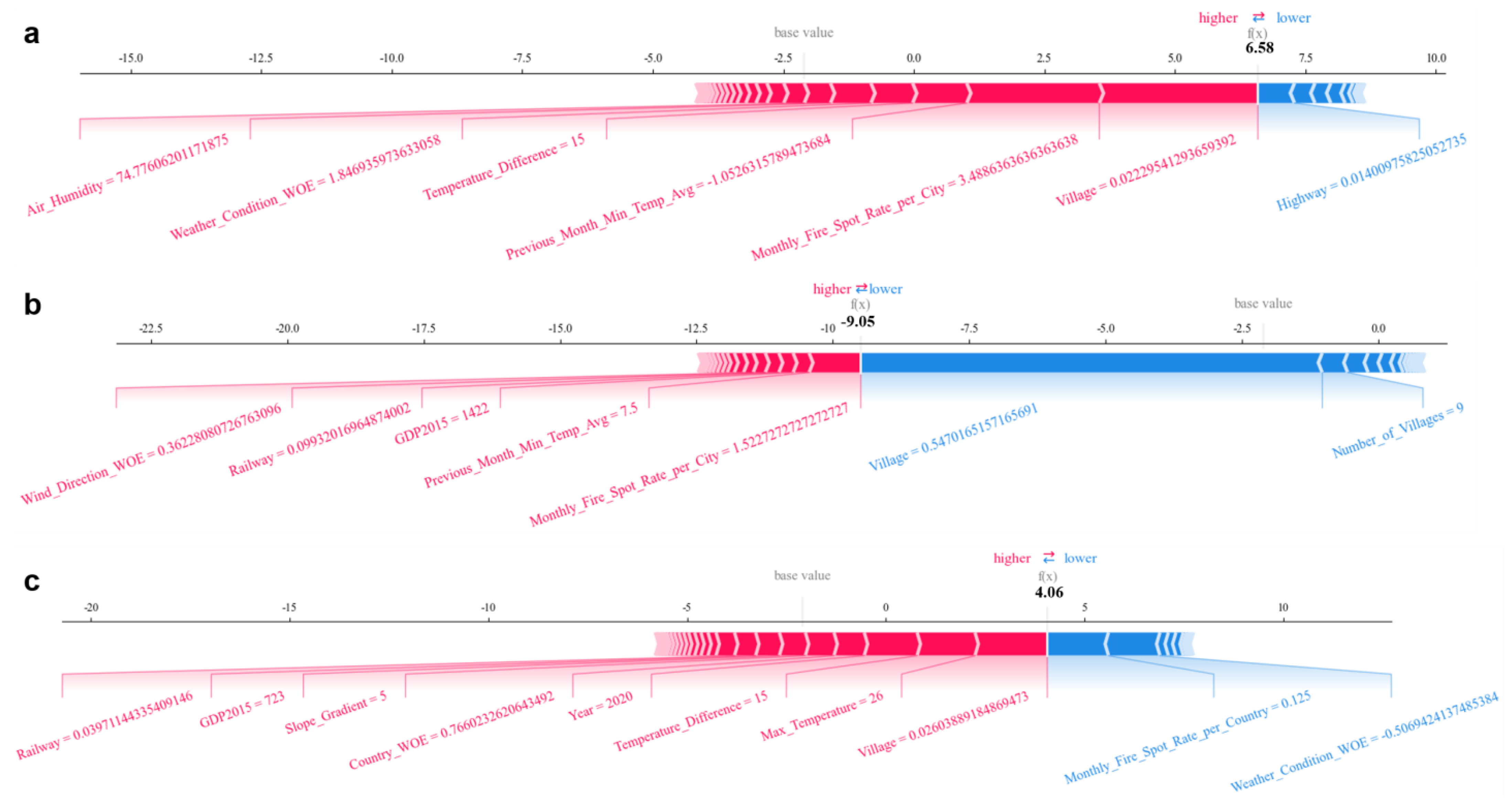
• Interpretability Analysis: Following model optimization, the SHAP (SHapley Additive exPlanations) framework is applied to enhance interpretability. SHAP decision and summary plots illustrate model predictions and identify key factors influencing wildfire occurrences. Dependence plots analyze feature−prediction relationships, while SHAP force plots provide detailed explanations for individual samples. This approach not only improves model transparency, but also offers empirical support for wildfire prevention and management. A detailed discussion of interpretability analysis is presented in Section 4.4.

4.3. Algorithm and Principles of the EWXS Model

This section details the application of the XGBoost algorithm to develop the EWXS model, with the objective of classifying and predicting wildfire occurrences. Let X = [x₁, x₂, …, x_n] ∈ R^n×d denote the input space encompassing topographic, human activity, and meteorological factors, where s represents the feature dimension, y = {y₀, y₁} signifies the output space, and the training dataset is $I=\left\{\right(x_1,y_1),\dots ,(x_n,y_n\left)\right\}$, with n indicating the sample size. The pseudocode for training the optimal model, BestEWXS, based on the XGBoost Algorithm 1 is as follows:

Algorithm 1. Pseudocode for training BestEWXS.

Training algorithm for the best prediction model BestEWXS

INPUT: Parameter 1: $\mathrm{training} \mathrm{data} I=\{\left(x_1,y_1\right);\left(x_2,y_2\right);\dots \dots ;(x_n,y_n\left)\right\}$ Parameter 2: Parameters of the EWXS algorithm OUTPUT: BestEWXS

$1\hspace{1em}I=\{\left(x_1,y_1\right);\left(x_2,y_2\right); \dots \dots ; (x_n,y_n\left)\right\}$ $2\hspace{1em} I\leftarrow x_i^{\mathrm{\prime }}={\displaystyle \frac{x_i-MIN\left(x_i\right)}{MAX\left(x_i\right)-MIN\left(x_i\right)}}$ $3\hspace{1em} I^{\mathrm{\prime }}\leftarrow$Missing Value Imputation(I) $4\hspace{1em} \tilde{I}\leftarrow WOE\left(I^{\mathrm{\prime }}\right)$ $5\hspace{1em} X\leftarrow$$\{x_1$$,x_2$$.,x_n$$\},y\leftarrow$$\{y_1$$,y_2$$.,y_n$} $6\hspace{1em} X_{train},{ X}_{test}, y_{train},{ y}_{test}$ = train_test_split(X, y, 0.3) $7\hspace{1em} D\leftarrow RandomOverSamplerg.fit\_resample(X_{train},y_{train})$ $8\hspace{1em} \mathrm{EWXS}\leftarrow \mathrm{X}\mathrm{G}\mathrm{B}\mathrm{o}\mathrm{o}\mathrm{s}\mathrm{t}(default\_parameters2)$ 9  max_iter ← Maximum number of iterations 10  for iteration in range(max_iter): 11   for each particle in the swarm: 12    Evaluate the accuracy of the particle’s current position 13    Update personal best position and global best position, if necessary 14   Update particle velocities and positions using PSO equations 15  Best_Parameter2 ← global_best_position $16\hspace{1em} \mathrm{BestEWXS} \leftarrow \mathrm{EWXS} (\mathrm{Best}\_\mathrm{Parameter}2).\mathrm{fit}(D$) 17 return BestEWXS

In line 1, the algorithm imports the raw data for wildfire prediction that has been previously constructed. Line 2 performs feature normalization to mitigate issues arising from varying scales. Line 3 utilizes XGBoost regression to impute missing values within the dataset. Line 4 encodes categorical variables to prepare the dataset for subsequent modeling. Lines 5 and 6 separate the features from the target variables in $\tilde{I}$ and subsequently partition the dataset into training and testing subsets at a 7:3 ratio. Specifically, 70% of the testing subset is further utilized for validation through five-fold cross-validation. Line 7 implements random oversampling on the training set to improve the model’s capacity to identify minority classes. Line 8 trains the initial model using default parameters (such as max_depth = 6, learning_rate = 0.3, n_estimators = 100, etc.). To identify the optimal model, lines 9 through 15 apply Particle Swarm Optimization (PSO) for hyperparameter tuning across five parameters. Line 9 sets the maximum number of iterations for the PSO algorithm. Line 10 initiates the iterative loop, while line 11 computes the accuracy for each particle within the swarm, identifying the global optimum, which is then assigned to “Best_Parameter2”. Lines 16–17 apply the best parameters to the model, generating the current best predictive model, BestEWXS, and replacing the initial model.

In the above algorithm, the XGBoost model utilized in line 8 plays a central role in the EWXS modeling process. XGBoost, introduced by Chen et al. [31], leverages CPU multithreading and parallel computation to significantly enhance classification accuracy. Its exceptional performance in wildfire prediction stems from its ability to process large, complex datasets and its built-in L1 and L2 regularization techniques, which effectively mitigate overfitting. This robustness makes XGBoost particularly well-suited for the dynamic and complex nature of wildfire environments. Furthermore, its capability to handle missing data during training provides a significant advantage when working with real-world datasets. The objective function of XGBoost is defined as follows:

$$Ob{j}^{\left(t\right)}=\sum _{i=1}^n l\left(y_i,{\widehat{y}}_i^{\left(t-1\right)}+f_t\left(x_i\right)\right)+\mathsf{\Omega }\left(f_t\right)$$

(1)

Here, l denotes the loss function; $y_i$ represents the actual value of the i-th sample; ${\widehat{y}}_i^{(t-1)}$ represents the predicted value after the t − 1 iteration; $f_t\left(x_i\right)$ represents the score function for the sample at the t-th iteration; and $\mathsf{\Omega }\left(f_t\right)$ represents the complexity of the tree. The calculation formula is as follows:

$$\mathsf{\Omega }\left(f\right)=\gamma T+{\displaystyle \frac{1}{2}}\lambda \sum _{j=1}^T w_j^2$$

(2)

In Equation (2), T represents the number of leaf nodes; γ and λ denote the regularization parameters; and $w_j$ represents the weight of the leaf node. The smaller the value of $\mathsf{\Omega }\left(f_t\right)$, the lower the complexity of the tree and the stronger its generalization ability.

Next, the Taylor expansion is used to approximate the objective function, ignoring higher-order infinitesimals and constant terms, resulting in the approximate objective function:

$$Ob{j}^{\left(t\right)}\approx \sum _{j=1}^T \left[\left(\sum _{i\in I_j} g_i\right)w_j+{\displaystyle \frac{1}{2}}\left(\sum _{i\in I_j} h_i+\lambda \right)w_j^2\right]+\gamma T$$

(3)

In Equation (3), $I_j=\left\{\begin{array}{c}i\mid q\left(x_i\right)=j\end{array}\right\}$ represents the set of instances in leaf node j; $g_i$ and $h_i$ denote the first and second-order derivatives of the loss function l with respect to the prediction value at t − 1 iterations, which are specifically calculated using Equations (4) and (5), respectively:

$$g_i={\displaystyle \frac{\partial l\left(y_i,y^{\left(t-1\right)}\right)}{\partial y^{\left(t-1\right)}}}$$

(4)

$$h_i={\displaystyle \frac{{\partial }^{2}l\left(y_i,y^{\left(t-1\right)}\right)}{\partial {\left(y^{\left(t-1\right)}\right)}^2}}$$

(5)

Next, by taking the partial derivative of $w_j$ in Equation (3) and setting it to 0, the optimal $w_j^{*}$ can be obtained. The specific calculation formula is as follows:

$$w_j^{\mathrm{*}}=-{\displaystyle \frac{\sum _{i\in I_j} g_i}{\sum _{i\in I_j} h_i+\lambda }}$$

(6)

Finally, define $G_j=\sum _{i\in I_j} g_i,H_j=\sum _{i\in I_j} h_i$, and substitute $w_j^{*}$ into Equation (3). After simplification, the optimal objective function can be obtained as follows:

$$Ob{j}^{\left(t\right)}=-{\displaystyle \frac{1}{2}}\sum _{j=1}^T {\displaystyle \frac{G_j^2}{H_j+\lambda }}+\gamma$$

(7)

4.4. Introduction to the SHapley Additive exPlanations (SHAP) Model

After successfully constructing the BestEWXS model, the SHAP (SHapley Additive exPlanations) methodology is employed to improve interpretability and address the model’s “black-box” nature. Proposed by Lundberg et al. [32], SHAP treats each feature as a “contributor” to the model’s predictions and quantifies its specific impact on the overall outcome.

SHAP is particularly valuable in revealing complex feature interactions, offering deeper insights into how various factors influence model predictions. A key advantage of SHAP is its ability to illustrate both positive and negative effects of each feature, providing a clear and interpretable explanation of the model’s decision-making process. This interpretability is crucial for understanding the underlying drivers of wildfire risk, enabling stakeholders to make well-informed decisions based on the model’s outputs.

Let $x_i$ be the i-th sample, $x_{ij}$ be the j-th feature of $x_i$, the model’s prediction for $x_i$ be ${\widehat{y}}_i$, and the mean prediction for training samples be $f_0$. The SHAP value satisfies the following equation:

$${\widehat{y}}_i=f_0+f\left(x_{i1}\right)+f\left(x_{i1}\right)+\dots +f\left(x_{ik}\right)$$

(8)

Here, $f\left(x_{ij}\right)$ is the SHAP value for $x_{ij}$, representing the contribution of the j-th feature of the i-th wildfire prediction sample to ${\widehat{y}}_i$. The SHAP values of different features represent the change in the prediction of the expected model due to that feature. The SHAP model applies a log-odds transformation to the XGBoost algorithm, as shown in Equation (9):

$$In\left({\displaystyle \frac{{\widehat{y}}_i}{1-{\widehat{y}}_i}}\right)=f_0+f\left(x_{i1}\right)+f\left(x_{i2}\right)+\dots +f\left(x_{ik}\right)$$

(9)

When $f\left(x_{ij}\right)>0$, it indicates that the feature has a positive effect on the prediction value; conversely, if $f\left(x_{ij}\right)<0$, it indicates a negative effect. The advantage of SHAP values lies in their ability to clearly display the positive and negative relationships of the impact and contribution of each feature in each sample, thus providing deeper insights for wildfire prediction.

5. Model Construction and Experimental Comparison

5.1. Experimental Environment and Evaluation Metrics

The experiments in this study were conducted on a Windows 10 operating system using Python 3.7. The hardware configuration included an Intel(R) Core (TM) i5-9300H processor with 8 GB of RAM. The software environment comprised PyCharm 2023.2 as the primary development tool and ArcMap 10.8 for spatial data processing.

To evaluate classification models, a confusion matrix provides an intuitive representation of the relationship between predicted and actual outcomes. This study employs accuracy (Acc), precision (Pre), recall, F1 score, and the area under the ROC curve (AUC) as evaluation metrics to comprehensively assess model performance. The definition of the confusion matrix is presented in

Table 5. Confusion matrix for prediction results.

Actual Condition	Predicted Outcome
	Wildfire Event Predicted	No Wildfire Predicted
Wildfire Event Occurred	True Positive (TP)	False Negative (FN)
Absence of Wildfire	False Positive (FP)	True Negative (TN)

.

$$Acc={\displaystyle \frac{TP+TN}{TP+TN+FP+FN}}$$

(10)

Accuracy (Acc) is defined as the proportion of correctly classified samples relative to the total number of samples. This metric provides an overall assessment of the classifier’s performance.

$$Pre={\displaystyle \frac{TP}{TP+FP}}$$

(11)

Precision (Pre), also referred to as Positive Predictive Value, is defined as the ratio of correctly identified wildfire samples to the total number of samples classified as wildfires by the model. This metric assesses the classifier’s predictive accuracy by indicating the proportion of true positives among all predicted positives.

$$Recall={\displaystyle \frac{TP}{TP+FN}}$$

(12)

Recall, often termed Sensitivity or True Positive Rate, is defined as the proportion of correctly identified positive samples relative to the total number of actual positive instances. This metric evaluates the classifier’s capability to detect all true positive cases, thus measuring its effectiveness in capturing genuine events. Specifically, in wildfire prediction, recall quantifies the number of actual wildfires successfully detected by the classifier. An increased recall value reflects a higher sensitivity of the classifier to identifying true wildfire occurrences.

$$F1={\displaystyle \frac{2\times Precision\times Recall}{Precision+Recall}}$$

(13)

The F1 score is a composite metric that harmonizes precision and recall by computing their harmonic mean. A higher F1 score signifies improved performance of the classifier, reflecting a balanced measure of both precision and recall.

The Area Under the Receiver Operating Characteristic (ROC) Curve (AUC) quantifies the area beneath the curve that plots recall rates against the false positive rates (1 − precision) across different threshold settings. An AUC value approaching 1 denotes exceptional classifier performance and enhanced classification capability.

5.2. Feature Engineering and Data Exploration and Analysis

To minimize the impact of varying feature scales on analytical results, this study applied min-max normalization to all features used in the nearest neighbor analysis. Min-max normalization rescales the features to a standard range, typically [0, 1], ensuring that all features contribute equally to the analysis, regardless of their original scales. This preprocessing step was performed before integrating fire point and non-fire point data, ensuring consistency and comparability across the dataset. The effects of normalization are visually illustrated in the three-dimensional t-SNE scatter plot in Figure 5a, which depicts the distribution of features after normalization.

In the consolidated dataset, some features contained missing values. Except for air humidity, variables with minimal missing data were excluded from the analysis. Given the strong correlation between air humidity and factors such as maximum temperature, minimum temperature, and altitude, the missing values for air humidity were imputed using the XGBoost model. Additionally, outliers marked as −9999 were removed, as this value in ArcGIS indicates incomplete data matching due to fire points or non-fire points being located near the borders of Guizhou Province, as shown in Figure 5b.

For discrete variables, this study applied the Weight of Evidence (WOE) [33] encoding method to transform categorical variables into WOE values, clarifying their relationship with the target variable. This approach not only streamlined the model-building process, but also improved the interpretability of feature importance, enabling a more precise assessment of each feature’s influence on wildfire risk. WOE encoding was specifically applied to discrete features such as city, weather conditions, wind direction, and vegetation type.

To further analyze the relationships among normalized features, a correlation heatmap was generated. This visualization illustrates the strength and direction of relationships between variables, aiding in the identification of potential multicollinearity and the influence of individual features on wildfire risk. Figure 5c presents the correlation heatmap, highlighting significant correlations between various features and the target variable, Fire_Spot. This analysis offers deeper insights into how different features interact and contribute to the overall model performance.

Following data cleaning, a joint kernel density estimation plot was used to further elucidate feature relationships and distributions (Figure 5d). The curve along the upper axis represents the distribution of the X-axis variable, while the curve along the right axis represents the distribution of the Y-axis variable. The central contour plot depicts the joint distribution of these variables. In the plot, blue regions indicate areas without fire occurrences, whereas orange regions represent areas where fires have occurred.

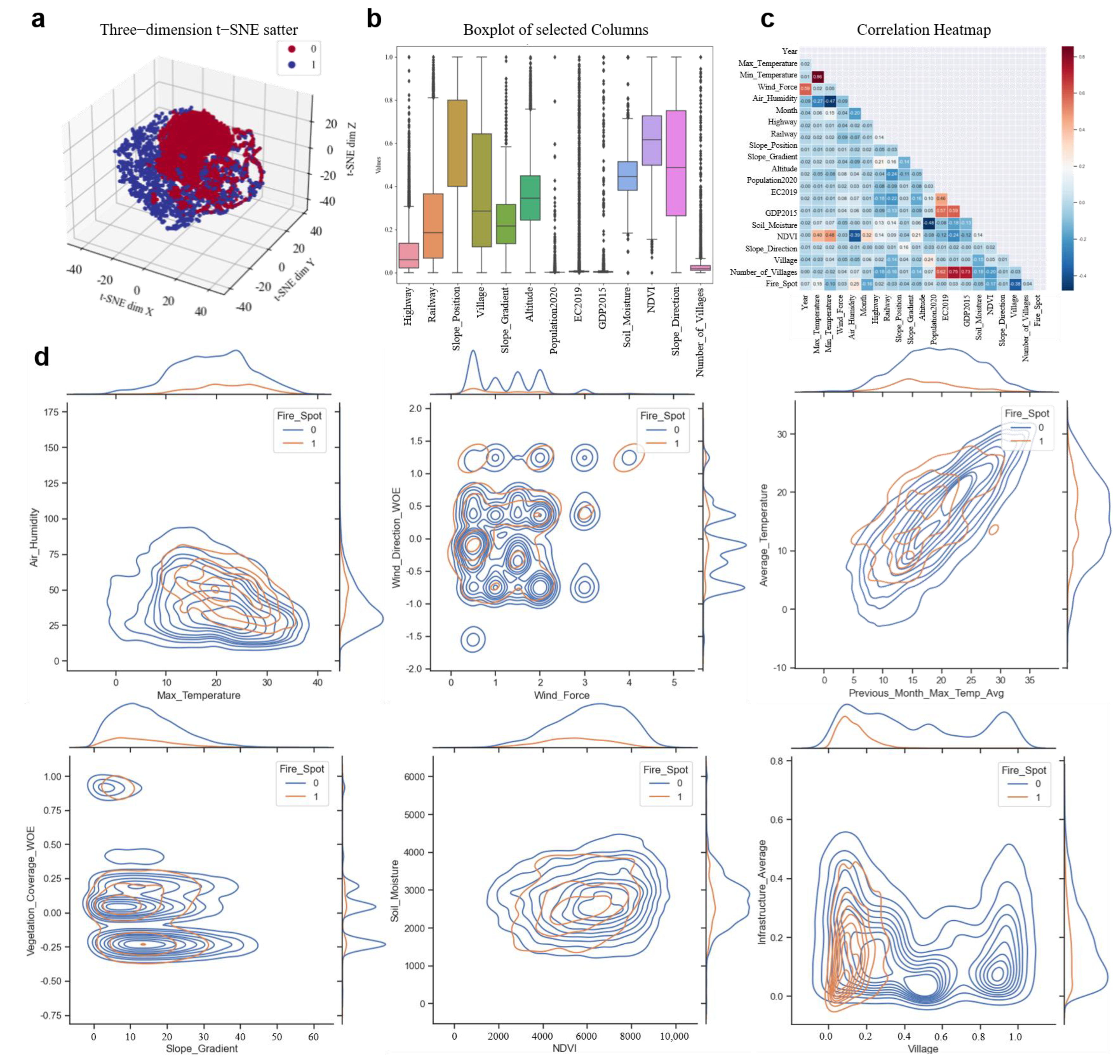
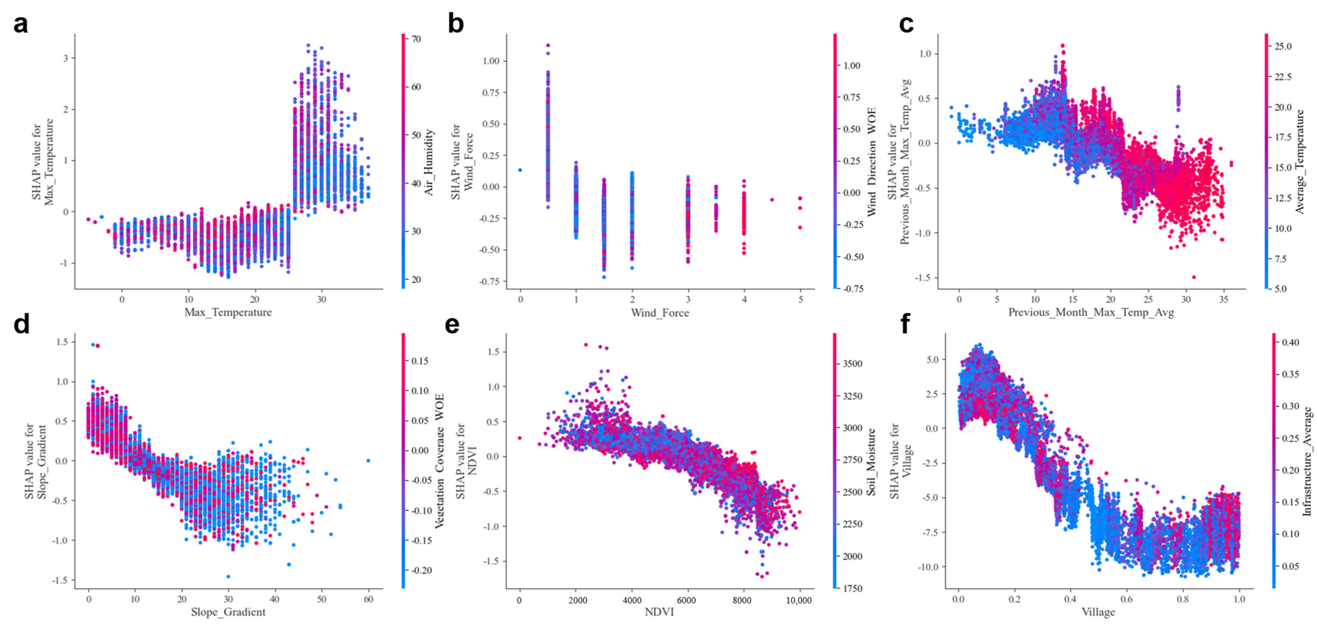
• Meteorological Factors: The joint distribution plot of air humidity and maximum temperature reveals that the likelihood of wildfire occurrence increases when both air humidity and temperature are elevated, with minimal overlap between the two. An analysis of wind speed and direction indicates that wildfires are more likely to occur in regions with lower wind speeds. Additionally, a comparison of the average maximum temperature from the previous month with the current month’s average temperature suggests that elevated temperatures increase the probability of wildfire occurrences.
• Geographic Factors: Joint distribution plots examining the relationship between slope and vegetation cover, as well as soil moisture and the Normalized Difference Vegetation Index (NDVI), suggest that topographic factors have a relatively minor role in wildfire prediction. This is supported by the observation that the peak values of contour lines remain largely unchanged regardless of fire occurrence.
• Human Activity Factors: Wildfires are more frequently observed near administrative villages. In contrast, proximity to infrastructure (such as railways and roads) has a lesser influence on fire occurrences.

In summary, human activities are the primary factors influencing wildfire occurrences, followed by meteorological factors, with geographic factors having a relatively minor impact.

5.3. Comparison of Imbalanced Data Handling Methods

In the wildfire prediction model, the dataset exhibits significant imbalance due to the lower frequency of wildfire events compared to non-wildfire events. This imbalance is a common challenge in predictive modeling, where minority class instances (wildfire events) are underrepresented, potentially biasing the model toward the majority class (non-wildfire events). To better reflect real-world conditions and ensure more accurate predictions, this study generated samples with a 1:5 ratio of non-wildfire to wildfire data, thus balancing the representation of both classes [30].

Common methods for addressing data imbalance include undersampling and oversampling [34]. Undersampling addresses the imbalance by reducing the number of non-wildfire samples, which, however, may lead to the loss of valuable information from the majority class. On the other hand, oversampling increases the number of wildfire samples by replicating existing instances or generating synthetic data through techniques such as SMOTE (Synthetic Minority Over Sampling Technique), which mitigates the risk of losing information but introduces the challenge of overfitting.

After data cleaning, this study applied several techniques to handle the imbalanced data: random undersampling, random oversampling, SMOTE, and its variants (such as Borderline-SMOTE and ADASYN). Random undersampling and oversampling were employed to adjust the class distribution, while SMOTE and its variants were used to generate synthetic instances of the minority class, improving the model’s ability to recognize patterns in the underrepresented wildfire events.

The performance of these preprocessing methods was then evaluated using the XGBoost model, a widely used algorithm for imbalanced classification tasks. By comparing the accuracy, precision, recall, and F1 score of each approach, we identified the most effective strategy for balancing the dataset and improving model performance. The results of these experiments are presented in

Table 6. Comparison of imbalanced data handling algorithms.

Imbalanced Data Handling Method	Accuracy	Precision	Recall	F1 Score	AUC	Overall
None	99.02%	98.39%	95.70%	97.02%	0.977	97.57%
Cluster Centroids	79.62%	44.89%	98.47%	61.65%	0.872	74.36%
SMOTE	98.86%	97.67%	95.44%	96.54%	0.975	97.20%
ADASYN	98.96%	97.53%	96.18%	96.85%	0.979	97.47%
Borderline SMOTE	98.98%	97.54%	96.30%	96.91%	0.979	97.53%
Random Under Sampler	96.43%	83.69%	97.72%	90.13%	0.970	92.98%
Random Over Sampler	99.03%	97.33%	96.82%	97.08%	0.982	97.68%

.

Table 6 demonstrates that oversampling techniques, including SMOTE, Borderline SMOTE, ADASYN, and Random Over Sampler, outperform the original, unprocessed dataset when applied to the XGBoost model. Notably, Random Over Sampler improved overall performance by 0.48%. In contrast, although Random Under Sampler enhanced recall, it led to a decrease in overall performance. These results suggest that oversampling methods are more effective in addressing the imbalance issue inherent in wildfire data.

5.4. Comparison with Existing Work

This section provides a comparative analysis of the performance of the EWXS model relative to several models reported in the literature, including deep learning models [7,23], Support Vector Machines (SVMs) [9], Gradient Boosting Decision Trees (GBDTs) [10], XGBoost [12], AdaBoost [13], and Random Forest [14,25]. The dataset was split in a 70:30 ratio, and five-fold cross-validation was applied. For all experiments, the random seed was fixed at 0. After parameter tuning, the EWXS model was configured with the following settings: learning rate = 0.465, maximum depth = 7, number of estimators = 94, number of bins = 107, and minimum child samples = 12. The performance evaluation results are summarized in

Table 7. Performance comparison of related research models.

Reference	Model	Accuracy	Precision	Recall	F1	AUC
Zhang H et al. [5]	Enhanced Regression Tree	89.3%	/	/	/	0.93
Xu S et al. [6]	BPNN	78.89%	78.86%	54.33%	/	0.793
Zhang J et al. [7]	Convolutional Neural Network	95%	90%	90%	/	0.838
Xi J et al. [8]	GBDT	95%	/	/	/	0.83
Cao L et al. [10]	Random Forest	93.80%	/	/	/	/
Pérez-Porras FJ et al. [11]	MLP		/	75%	60%	/
Dong H et al. [12]	XGB	81.32%	/	/	78.62%	0.805
Qiu L et al. [26]	Random Forest	/	/	/	/	0.98
Rubí J N S et al. [13]	AdaBoost	/	/	/	/	0.993
Nur A S et al. [9]	SVR-PSO	/	/	/	/	0.882
Abdollahi A et al. [24]	Deep Learning Model	93%	/	/	/	0.91
Tavakkoli Piralilou S et al. [14]	Random Forest	92.5%	/	/	/	0.947
Ours	BestEWXS	99.22%	98.48%	96.82%	97.64%	0.983

.

Table 7 shows that the BestEWXS model significantly outperforms existing models across several key evaluation metrics. Specifically, the model achieves an accuracy of 99.22%, precision of 98.48%, recall of 96.82%, F1 score of 97.64%, and AUC value of 0.983. Existing models struggle with complex feature interactions, fail to address imbalanced data processing, and underutilize features, leading to subpar performance. In contrast, the BestEWXS model demonstrates substantial improvements in all evaluation metrics. Accuracy increases from 4.22% to 20.33%, precision rises from 8.48% to 19.62%, recall improves from 6.82% to 21.82%, and the F1 score shows the largest improvement, ranging from 19.02% to 37.64%. These results not only confirm the effectiveness of the BestEWXS model, but also highlight its superior performance in wildfire prediction.

The significant improvements in all evaluation metrics for the BestEWXS model can be attributed to two key factors:

• Multi-Source Data Integration: This study developed a comprehensive dataset by integrating vector data, raster data, and structured tabular data from diverse sources. Specifically, non-wildfire samples were generated at a 1:5 ratio to enhance the model’s ability to detect fire events. Key factors such as distance to villages, temperature variations, and air humidity provided critical information for predicting wildfire risk.
• Imbalanced Data Handling: After data integration, the study employed random oversampling techniques to address the issue of data imbalance. This approach increased the number of fire samples, thereby improving the model’s accuracy in predicting the minority class (i.e., fire events).

5.5. Comparison with Mainstream Machine Learning Models

To thoroughly evaluate the performance of the EWXS model, this section compares it with various mainstream machine learning models. After feature engineering, the data were randomly split into training and testing sets with a 70:30 ratio to ensure the robustness of the results. Specifically, 70% of the testing subset was further used for validation through five-fold cross-validation. The experiments initialized the random seed to 0 and applied five-fold cross-validation to mitigate the effects of model randomness. The performance metrics of the models are presented in

Table 8. Performance comparison of different mainstream models.

Model Name	Accuracy	Precision	Recall	F1 Score	AUC	Average
Logistic	60.58%	23.12%	59.03%	33.23%	0.600	47.19%
KNC	71.05%	32.15%	66.85%	43.41%	0.694	56.57%
Naive Bayes	55.73%	22.60%	67.57%	33.70%	0.605	48.02%
DTC	96.81%	90.10%	90.80%	90.44%	0.944	92.51%
MLPC	71.13%	33.38%	49.90%	27.71%	0.626	48.94%
GBDT	95.38%	80.10%	96.11%	87.37%	0.957	90.93%
RF	98.13%	96.02%	92.59%	94.27%	0.959	95.38%
ETC	98.03%	98.25%	89.75%	93.80%	0.947	94.91%
AdaBoost	92.06%	69.72%	92.44%	79.48%	0.922	85.18%
HGBC	98.63%	95.09%	96.75%	95.91%	0.979	96.86%
Ridge	87.20%	56.99%	93.94%	70.93%	0.899	79.79%
SVM	78.88%	23.14%	11.67%	15.50%	0.520	36.24%
LGBM	98.74%	95.79%	96.67%	96.23%	0.979	97.07%
EWXS	99.03%	97.33%	96.82%	97.08%	0.982	97.69%

.

The results presented in Table 8 demonstrate that the EWXS model outperforms other mainstream machine learning models across all performance metrics. Specifically, the EWXS model achieves an accuracy of 98.63%, precision of 95.09%, recall of 96.75%, an F1 score of 95.91%, and an AUC value of 0.979. However, models such as Logistic Regression, KNN, Naive Bayes, and SVM underperformed in our study. Logistic Regression struggled with non-linear relationships, KNN performed poorly on high-dimensional and imbalanced data, Naive Bayes failed due to its assumption of feature independence, and SVM faced high computational costs and sensitivity to class imbalance—factors that reduced their effectiveness in wildfire prediction. For instance, compared to the Naive Bayes model, EWXS improved overall performance by 25.29%, underscoring the presence of complex non-linear relationships in the data.

In comparison to the Gradient Boosting Decision Trees (GBDTs), Random Forest, AdaBoost, and Support Vector Machine (SVM) models documented in the literature [9,10,13,14,25], the EWXS model demonstrates improvements ranging from 0.9% to 20.15% in accuracy, 1.31% to 74.19% in precision, 4.23% to 85.15% in recall, 2.81% to 81.58% in F1 score, and 0.06 to 0.462 in AUC. Additionally, Figure 6a illustrates the Reliability Curve, with the yellow line representing the EWXS model, which outperforms the other models. The Lift Curve in Figure 6b further highlights the ability of EWXS to identify positive samples across varying sample percentages, showing a significant improvement over random selection. Furthermore, Figure 6c presents the Cumulative Gain Plot, which demonstrates the EWXS model’s capacity to capture a higher proportion of positive samples within the top percentage of predictions compared to the other models. This plot confirms that EWXS consistently outperforms other algorithms by yielding a greater cumulative gain, thereby validating its effectiveness in detecting positive cases. The superior performance of the EWXS model across these five metrics can be attributed to several factors: XGBoost includes regularization terms that effectively manage model complexity and mitigate overfitting. Additionally, its parallel processing capabilities significantly accelerate training on large-scale datasets. The adaptable loss function framework of XGBoost is also applicable to a wide range of predictive problems, further demonstrating its broad applicability and superior predictive accuracy.

5.6. Hyperparameter Optimization and Generalization Ability Analysis

To determine the optimal configuration of the EWXS model, this study utilized a Particle Swarm Optimization (PSO) algorithm [23], with accuracy as the objective function, to fine-tune five key hyperparameters of the XGBoost base model. These hyperparameters include the learning rate (learning_rate), maximum depth (max_depth), number of base learners (n_estimators), number of bins (n_bins), and the minimum number of samples per child node (min_child_samples). The search ranges and tuning values for these hyperparameters are provided in

Table 9. Model hyperparameter tuning.

Hyperparameter	Range of Values	Optimized Value	Description of the Parameter
learning_rate	[0.001, 0.5]	0.465	Learning Rate
max_depth	[2, 50]	7	Maximum Depth
n_estimators	[0, 100]	94	Number of Base Estimators
n_bins	[2, 256]	107	Number of Bins
min_child_samples	[1, 50]	12	Minimum Samples per Leaf

.

Table 10. Performance comparison before and after hyperparameter tuning.

	Accuracy	Precision	Recall	F1 Score	AUC
EWXS	99.03%	97.33%	96.82%	97.08%	0.982
BestEWXS	99.22%	98.48%	96.82%	97.64%	0.983

presents a comparative analysis of the EWXS model’s performance before and after hyperparameter tuning, which was optimized through 500 swarm iterations. The results indicate that the optimized BestEWXS model outperforms the original model across four performance metrics, with the exception of recall. Specifically, the AUC value showed a marginal increase of 0.001, while other performance metrics improved from 0.18% to 1.15%, with precision showing the most significant enhancement. These findings highlight that hyperparameter tuning has significantly improved the model’s accuracy in forecasting wildfire occurrences.

In addition to evaluating the model’s predictive performance using the test set, it is essential to assess its generalization ability. To achieve this, the study employed learning curves to examine the model’s performance across the entire dataset. Figure 6d provides a comparative analysis of the learning curves for AdaBoost, SVM, Decision Tree, Gradient Boosting, Random Forest, and the EWXS model.

The learning curves in Figure 6d illustrate how each model’s performance varies with changes in sample size. The results show that, with the exception of the SVM model, all other models demonstrated improved fitting performance as the sample size increased. The SVM model exhibited signs of underfitting, while the EWXS and other tree-based models maintained stable performance as the sample size grew. Although the EWXS model experienced a slight decline when the sample size reached 7000, it exhibited more robust performance with 8000 samples. This suggests that the EWXS model effectively controls model complexity through regularization, thereby mitigating overfitting and enhancing its generalization ability.

6. Interpretability Analysis

Building upon the EWXS model developed in Section 4, this section uses the SHAP framework to conduct a comprehensive analysis of the factors influencing wildfire occurrences. This analysis includes the use of summary plots, decision plots, and dependence plots. Additionally, SHAP force plots are employed to investigate the relationships between various factors and within individual samples.

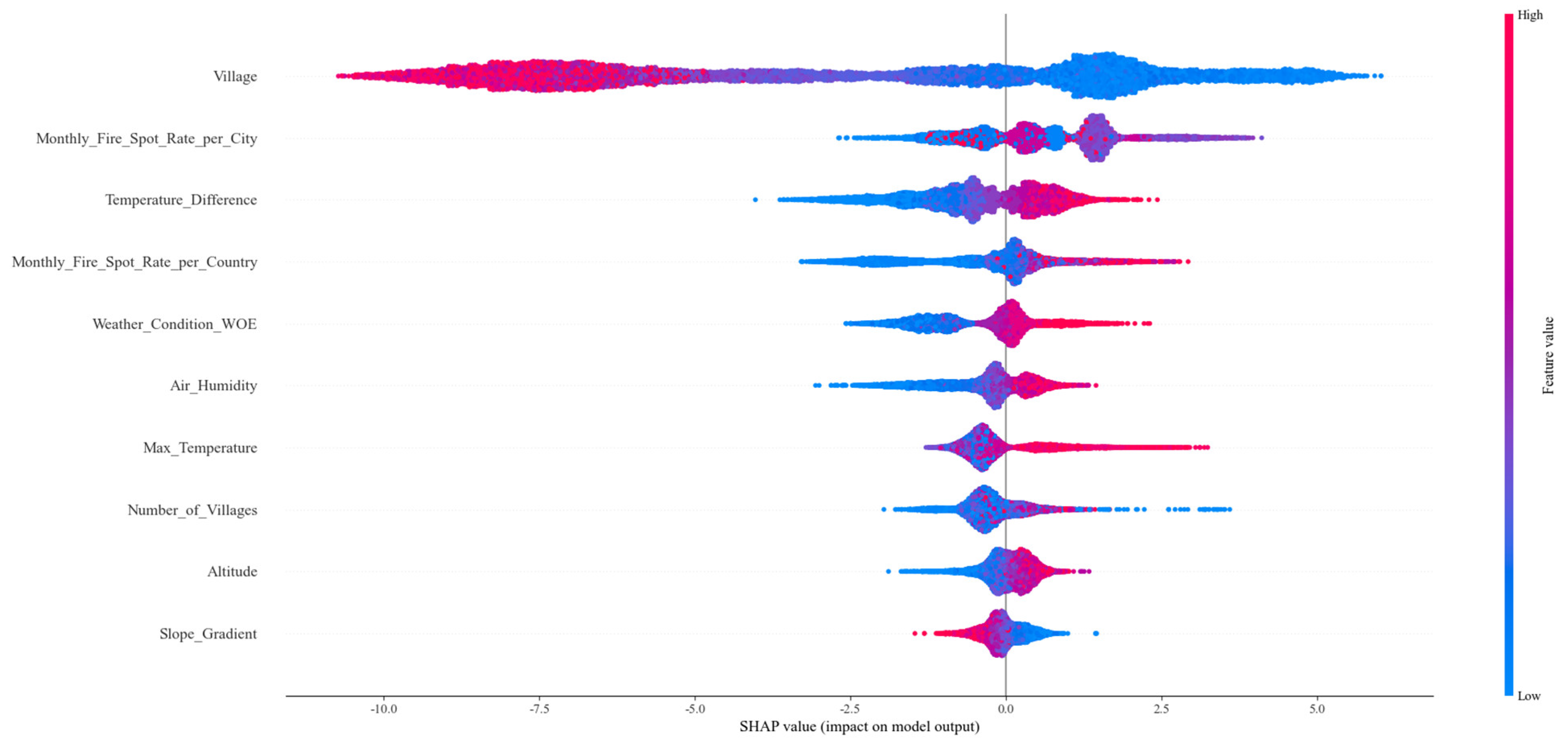
6.1. Feature Importance Comparison Analysis

The SHAP summary plot for the EWXS model highlights the contribution of key features to the prediction outcomes. In the plot, color intensity represents the magnitude of feature values, with the horizontal axis showing SHAP values and the vertical axis representing feature names.

Figure 7 presents the ten most influential features, which include Distance to Administrative Village (Village), Monthly Average Fire Spot Rate in the City (Monthly_Fire_Spot_Rate_pre_City), Temperature Difference (Temperature_Difference), Monthly Average Fire Spot Rate in the County (Monthly_Fire_Spot_Rate_pre_Country), Weather Condition (Weather_Condition_WOE), Air Humidity (Air_Humidity), Maximum Temperature (Max_Temperature), Number of Surrounding Administrative Villages (Number_of_Village), Altitude (Altitude), and Slope Gradient (Slope_Gradient).

To better illustrate the contributions of various factors to wildfire prediction, decision plots were generated, as shown in Figure 8, based on the analysis in Figure 7.

In Figure 8, the colored lines represent the behavior of individual samples in relation to the prediction outcome. Each colored line corresponds to the contribution of a single sample’s feature as it varies across different feature values. The position of these lines relative to the gray baseline indicates the impact of the features on the prediction for each sample.

The colored lines reflect the individual contributions of a particular sample. For each feature, the line demonstrates how its value influences the model’s output as the feature value changes. The gradient of the line reflects the magnitude of this impact.

The gray line represents the model’s baseline prediction. When a colored line is above the baseline, it indicates that the feature value positively contributes to the predicted outcome. Conversely, if the line is below the baseline, it suggests a negative contribution to the prediction. The analysis of feature categories is provided below:

• Figure 8a Meteorological Factors: Temperature Difference (Temperature_Difference), Weather Condition (Weather_Condition_WOE), Air Humidity (Air_Humidity), and Maximum Temperature (Max_Temperature) are positively correlated with wildfire risk. Specifically, increases in these factors raise the likelihood of fire occurrence. Additionally, the minimum temperature and weather conditions from the previous month significantly influence wildfire risk.
• Figure 8b Human Activity Factors: Distance to Towns and Villages (Village), Monthly Average Fire Spot Rate in the City (Monthly_Fire_Spot_Rate_pre_City), and Monthly Average Fire Spot Rate in the County (Monthly_Fire_Spot_Rate_pre_Country) exhibit a negative correlation with wildfire risk. Greater distances from villages are associated with reduced fire risk, while regions with a history of frequent fires have a higher risk of future fires. Notably, the variable “Village” plays a particularly prominent role in the decision plot, underscoring its critical importance in predicting wildfire risk.
• Figure 8c Geographical Factors: Among the geographical factors, Altitude (Altitude) and Slope Gradient (Slope_Gradient) significantly affect wildfire risk. Increased altitude raises fire risk, while reduced slope gradients also contribute to higher fire risk. Furthermore, the Normalized Difference Vegetation Index (NDVI) and Soil Moisture (Soil_Moisture) are crucial factors in fire prediction.

6.2. Feature Dependence Analysis

To gain deeper insights into how variations in key feature values affect the EWXS model’s predictions of wildfire occurrences, SHAP feature summary plots were used. Meteorological factors selected for this analysis include Temperature Difference (Max_Temperature), Wind Speed (Wind_Force), and the Previous Month’s Average Maximum Temperature (Previous_Month_Max_Temp_Avg). From the geographical factors, Slope Gradient (Slope_Gradient) and the Normalized Difference Vegetation Index (NDVI) were chosen, along with Village Distance (Village) from human activity factors. The SHAP dependence plots are shown in Figure 9. Specifically, Figure 9a–c displays interactions among meteorological factors, Figure 9d,e depicts interactions among geographical factors, and Figure 9f illustrates interactions among features related to human activity.

In the SHAP dependence plots, the horizontal axis represents the range of values for each feature, the vertical axis indicates the corresponding SHAP values, and the third dimension illustrates feature interactions. The analysis is organized into three primary categories: meteorological factors, geographical factors, and human activity factors.

6.3. Sample Decision Process Analysis

In addition to examining the general factors influencing wildfires, the SHAP framework can analyze factors at the sample level. This section selects samples with or without fire incidents, as well as those with prediction errors, to investigate variations in influencing factors.

Figure 10a presents a SHAP force plot for a randomly selected sample predicted to experience a wildfire. Features highlighted in red contribute positively to the model’s prediction, indicating that these factors increase fire risk. Key factors include a distance of 0.3 km to administrative villages (normalized to 0.0223), as discussed in Section 6.2, where distances less than 2.7 km typically correspond to higher fire risk. Additionally, meteorological factors—such as an average minimum temperature of −1.05 °C from the previous month, a temperature difference of 15 °C on the day of the sample, and an average of 3.5 fires per month in the vicinity—are significant contributors to wildfire occurrence. However, the distance to the road negatively impacts the likelihood of fire in this sample. Notably, the factors influencing fire occurrence in this case are predominantly related to human activity and meteorological conditions, with geographical factors contributing less.

Figure 10b illustrates the SHAP force plot for a sample predicted not to experience a wildfire. Features depicted in blue have a negative contribution to the prediction, indicating a decrease in fire risk. Key factors include a distance of 7.3 km from villages (normalized to 0.547), suggesting that areas farther from villages face a lower fire risk. Additionally, the presence of only nine villages within a 5 km radius contributes to the absence of fire events. These factors underscore the critical role of human activity in wildfire prevention.

Figure 10c shows the misclassified samples, where the true label was “no wildfire”, but the model predicted “wildfire”. Key factors contributing to this misclassification include a distance of 0.311 km to the administrative village (normalized to 0.026). As noted in the previous analysis, distances less than 2.7 km typically indicate a higher wildfire risk. Additionally, higher temperatures and greater temperature differences contributed to the misclassification as a wildfire. These three features were responsible for the incorrect prediction.

7. Discussion

In recent years, the application of machine learning models in natural disaster risk prediction has become a prominent research focus. Building on the XGBoost algorithm, this study proposes a machine learning model named EWXS, which aims to precisely predict wildfire occurrence risks and identify the key influencing factors.

The experimental results demonstrate that the EWXS model significantly outperforms multiple models proposed in the existing literature in terms of prediction performance. These models include the Enhanced Regression Tree [5], Backpropagation Neural Network [6], Convolutional Neural Network [7], Gradient Boosting Decision Tree [8], Support Vector Machine [9], Random Forest [10], Multilayer Perceptron [11], XGBoost [12], AdaBoost [13], and Deep Learning Model [14]. This conclusion has been validated through rigorous performance evaluations in Section 5.3.

Regarding variable selection, this study constructs 21 feature variables by integrating multi-source heterogeneous data, covering four major categories: geographical factors, meteorological factors, human activity factors, and others. Compared to similar XGBoost-based models [12], this study adds eight new feature variables, significantly enhancing the model’s prediction performance.

Existing research indicates that an increase in altitude leads to a significant reduction in wildfire probability. This is primarily due to higher vegetation and soil moisture in high-altitude areas and less interference from human activities [35], both of which are unfavorable for fire occurrence. Meteorological conditions mainly regulate the spatiotemporal distribution of wildfires by affecting the moisture content and temperature of combustibles. Specifically, an increase in temperature reduces the moisture content of combustibles and raises their temperature, thereby reducing the energy required for an external heat source to reach the ignition point and increasing fire risk. In contrast, an increase in precipitation saturates the moisture content of combustibles, significantly reducing the likelihood and severity of fires.

Moreover, the impact of human activities on wildfires cannot be ignored. Research shows that the farther the distance from human activity areas, the lower the probability of fire occurrence [36]. The findings of this study are highly consistent with the aforementioned literature. Additionally, this study introduces new feature variables, such as temperature difference, weather conditions, month, and slope, and conducts quantitative analyses on them. For example, it was found that the fire risk peaks within a 0–2.7 km radius of villages, then gradually decreases with increasing distance and stabilizes beyond 8.07 km. The detailed analysis results are presented in Section 6.

8. Conclusions and Future Work

Accurate wildfire prediction is crucial for safeguarding public safety, preserving ecological balance, mitigating disaster risks, enhancing emergency response efficiency, and promoting societal awareness of preventive measures. This study introduces an explainable wildfire prediction model based on Extreme Gradient Boosting (XGBoost), termed EWXS, designed to improve the accuracy and efficiency of early wildfire warning systems and provide scientific decision support for fire prevention and emergency management.

Initially, this study employed Weight of Evidence (WOE) encoding, missing value imputation techniques, and random oversampling to address data imbalance in the wildfire dataset. Building on this foundation, the EWXS prediction model was constructed using the XGBoost algorithm and rigorously compared with 10 existing models, including mainstream models such as Random Forest, CatBoost, and LightGBM. The comparative results demonstrate that the EWXS model significantly outperforms other models across multiple key performance metrics. Additionally, the Particle Swarm Optimization algorithm was applied to fine-tune the model’s hyperparameters, with accuracy as the objective function, resulting in notable improvements in key performance indicators.

Furthermore, this study utilized the SHAP framework to conduct a detailed analysis of the factors influencing the model, identifying key features that impact wildfire occurrence, such as distance to villages, weather conditions, air humidity, and vegetation temperature differences. The results show that the EWXS model not only offers exceptional predictive performance, but also provides substantial interpretability, delivering significant practical value in enhancing the accuracy of wildfire prediction.

Future research will focus on expanding the scope of data sample collection, extending both the temporal range and spatial coverage of the samples, and further improving the model’s predictive performance. Additionally, we will track and update the research data to analyze the latest wildfire trends and changes in influencing factors.

References

- Wei, J.; Li, Z.; Ma, Z.; Wang, H.; Wang, Q.; Shu, L.; Yang, Y.; Gao, Z. Spatiotemporal Clustering Analysis of Forest Fires in Yunnan Province. Fire Sci. Technol. 2020, 39, 1425–1429. [Google Scholar]
- Ponomarev, E.; Yakimov, N.; Ponomareva, T.; Yakubailik, O.; Conard, S.G. Current trend of carbon emissions from wildfires in Siberia. Atmosphere 2021, 12, 559. [Google Scholar] [CrossRef]
- Tükenmez, İ.; Özkan, Ö. Matheuristic approaches for multi-visit drone routing problem to prevent forest fires. Int. J. Disaster Risk Reduct. 2024, 112, 104776. [Google Scholar] [CrossRef]
- Zaidi, A. Predicting wildfires in Algerian forests using machine learning models. Heliyon 2023, 9, e18064. [Google Scholar] [CrossRef]
- Zhang, H.; Li, H.; Zhao, P.W. Risk of forest fire occurrence in Inner Mongolia and the impact of its drivers. Acta Ecol. Sin. 2024, 44, 5669–5683. [Google Scholar]
- Xu, S.; Xu, J.; Qu, K.; Yang, J.; Zhou, C. Fire prediction algorithm based on improved neighborhood rough set and optimized BPNN. J. Nanjing Univ. Sci. Technol. 2024, 48, 192–201. [Google Scholar]
- Zhang, J.; Peng, D.; Zhang, C.; He, D.; Yang, C. Research on fire prediction modeling in the Greater Khingan Range of Inner Mongolia based on deep learning. For. Sci. Res. 2024, 37, 31–40. [Google Scholar]
- Xi, J.; Fu, W. Watershed-scale forest fire risk prediction based on machine learning. J. Nat. Disasters 2024, 33, 89–98. [Google Scholar]
- Nur, A.S.; Kim, Y.J.; Lee, J.H.; Lee, C.W. Spatial prediction of wildfire susceptibility using hybrid machine learning models based on support vector regression in Sydney, Australia. Remote Sens. 2023, 15, 760. [Google Scholar] [CrossRef]
- Cao, L.; Liu, X.; Chen, X.; Yu, M.; Xie, W.; Shan, Z.; Gao, B.; Shan, Y.; Yu, B.; Cui, C. Prediction Model of Forest Fire Occurrence Probability in Yanbian Area, Jilin Province. J. Northeast For. Univ. 2024, 52, 90–96. [Google Scholar]
- Pérez-Porras, F.J.; Triviño-Tarradas, P.; Cima-Rodríguez, C.; Meroño-de-Larriva, J.E.; García-Ferrer, A.; Mesas-Carrascosa, F.J. Machine learning methods and synthetic data generation to predict large wildfires. Sensors 2021, 21, 3694. [Google Scholar] [CrossRef]
- Dong, H.; Wu, H.; Sun, P.; Ding, Y. Wildfire Prediction Model Based on Spatial and Temporal Characteristics: A Case Study of a Wildfire in Portugal’s Montesinho Natural Park. Sustainability 2022, 14, 10107. [Google Scholar] [CrossRef]
- Rubí, J.N.S.; Gondim, P.R. A performance comparison of machine learning models for wildfire occurrence risk prediction in the Brazilian Federal District region. Environ. Syst. Decis. 2023, 44, 351–368. [Google Scholar] [CrossRef]
- Tavakkoli Piralilou, S.; Einali, G.; Ghorbanzadeh, O.; Nachappa, T.G.; Gholamnia, K.; Blaschke, T.; Ghamisi, P. A Google Earth Engine approach for wildfire susceptibility prediction fusion with remote sensing data of different spatial resolutions. Remote Sens. 2022, 14, 672. [Google Scholar] [CrossRef]
- Radke, D.; Hessler, A.; Ellsworth, D. FireCast: Leveraging Deep Learning to Predict Wildfire Spread. In Proceedings of the Twenty-Eighth International Joint Conference on Artificial Intelligence (IJCAI-19), Macao, 10–16 August 2019; pp. 4575–4581. [Google Scholar]
- Pereira, J.; Mendes, J.; Júnior, J.S.; Viegas, C.; Paulo, J.R. A review of genetic algorithm approaches for wildfire spread prediction calibration. Mathematics 2022, 10, 300. [Google Scholar] [CrossRef]
- Wang, S.S.-C.; Qian, Y.; Leung, L.R.; Zhang, Y. Identifying Key Drivers of Wildfires in the Contiguous US Using Machine Learning and Game Theory Interpretation. Earth’s Future 2021, 9, e2020EF001910. [Google Scholar] [CrossRef]
- Ban, Y.; Zhang, P.; Nascetti, A.; Bevington, A.R.; Wulder, M.A. Near real-time wildfire progression monitoring with Sentinel-1 SAR time series and deep learning. Sci. Rep. 2020, 10, 1322. [Google Scholar] [CrossRef]
- Jaafari, A.; Zenner, E.K.; Panahi, M.; Shahabi, H. Hybrid artificial intelligence models based on a neuro-fuzzy system and metaheuristic optimization algorithms for spatial prediction of wildfire probability. Agric. For. Meteorol. 2019, 266, 198–207. [Google Scholar] [CrossRef]
- Song, Y.; Wang, Y. Global wildfire outlook forecast with neural networks. Remote Sens. 2020, 12, 2246. [Google Scholar] [CrossRef]
- Bustillo Sánchez, M.; Tonini, M.; Mapelli, A.; Fiorucci, P. Spatial assessment of wildfires susceptibility in Santa Cruz (Bolivia) using random forest. Geosciences 2021, 11, 224. [Google Scholar] [CrossRef]
- Riaz, M.T.; Riaz, M.T.; Rehman, A.; Bindajam, A.A.; Mallick, J.; Abdo, H.G. An integrated approach of support vector machine (SVM) and weight of evidence (WOE) techniques to map groundwater potential and assess water quality. Sci. Rep. 2024, 14, 26186. [Google Scholar] [CrossRef]
- Kennedy, J.; Eberhart, R. Particle swarm optimization. inproceedings of icnn’95-international conference on neural networks 1995. IEEE. View Article. 1995, 4, 1942–1948. [Google Scholar]
- Abdollahi, A.; Pradhan, B. Explainable artificial intelligence (XAI) for interpreting the contributing factors feed into the wildfire susceptibility prediction model. Sci. Total Environ. 2023, 879, 163004. [Google Scholar] [CrossRef]
- Sakellariou, S.; Sfougaris, A.; Christopoulou, O. Integrated wildfire risk assessment of natural and anthropogenic ecosystems based on simulation modeling and remotely sensed data fusion. Int. J. Disaster Risk Reduct. 2022, 78, 103125. [Google Scholar]
- Qiu, L.; Chen, J.; Fan, L.; Sun, L.; Zheng, C. High-resolution map of wildfire drivers in California based on machine learning. Sci. Total Environ. 2022, 833, 155155. [Google Scholar] [CrossRef]
- Zhao, W.; Lu, X.; Chen, Q. The impact of topography on soil properties and soil type distribution in the limestone area of Guizhou. Chin. Soil Fertil. 2023, 1, 1–13. [Google Scholar]
- Zhang, Y.L.; Tian, L.L.; Ding, B.; Zhang, Y.W.; Liu, X.; Wu, Y. Driving factors and prediction model of forest fire in Guizhou Province. Chin. J. Ecol. 2024, 43, 282–289. [Google Scholar]
- Calkin, D.E.; Cohen, J.D.; Finney, M.A.; Thompson, M.P. How risk management can prevent future wildfire disasters in the wildland-urban interface. Proc. Natl. Acad. Sci. USA 2014, 111, 746–751. [Google Scholar] [CrossRef]
- Johnson, J.M.; Khoshgoftaar, T.M. Survey on deep learning with class imbalance. J. Big Data 2019, 6, 27. [Google Scholar] [CrossRef]
- Chen, T.; Guestrin, C. Xgboost: A scalable tree boosting system. In Proceedings of the 22nd ACM SIGKDD International Conference on Knowledge Discovery and Data Mining, San Francisco, CA, USA, 13–17 August 2016; pp. 785–794. [Google Scholar]
- Lundberg, S.M.; Lee, S.I. A unified approach to interpreting model predictions. Adv. Neural Inf. Process. Syst. 2017, 30, 4765–4774. [Google Scholar]
- Ji, S.; Li, J.; Du, T.; Li, B. Survey on Techniques, Applications and Security of Machine Learning Interpretability. J. Comput. Res. Dev. 2019, 56, 2071–2096. [Google Scholar]
- Wang, L.; Han, M.; Li, X.; Zhang, N.; Cheng, H. Review of classification methods on unbalanced data sets. IEEE Access 2021, 9, 64606–64628. [Google Scholar] [CrossRef]
- Vilar, L.; Woolford, D.G.; Martell, D.L.; Martín, M.P. A model for predicting human-caused wildfire occurrence in the region of Madrid, Spain. Int. J. Wildland Fire 2010, 19, 325–337. [Google Scholar] [CrossRef]
- Jaafari, A.; Rahmati, O.; Zenner, E.K.; Mafi-Gholami, D. Anthropogenic activities amplify wildfire occurrence in the Zagros eco-region of western Iran. Nat. Hazards 2022, 114, 457–473. [Google Scholar] [CrossRef]