Abstract
Black locust (Robinia pseudoacacia L.) is a tree species of high economic and ecological value, but is also considered to be highly invasive. Understanding the global potential distribution and ecological characteristics of this species is a prerequisite for its practical exploitation as a resource. Here, a maximum entropy modeling (MaxEnt) was used to simulate the potential distribution of this species around the world, and the dominant climatic factors affecting its distribution were selected by using a jackknife test and the regularized gain change during each iteration of the training algorithm. The results show that the MaxEnt model performs better than random, with an average test AUC value of 0.9165 (±0.0088). The coldness index, annual mean temperature and warmth index were the most important climatic factors affecting the species distribution, explaining 65.79% of the variability in the geographical distribution. Species response curves showed unimodal relationships with the annual mean temperature and warmth index, whereas there was a linear relationship with the coldness index. The dominant climatic conditions in the core of the black locust distribution are a coldness index of −9.8 °C–0 °C, an annual mean temperature of 5.8 °C–14.5 °C, a warmth index of 66 °C–168 °C and an annual precipitation of 508–1867 mm. The potential distribution of black locust is located mainly in the United States, the United Kingdom, Germany, France, the Netherlands, Belgium, Italy, Switzerland, Australia, New Zealand, China, Japan, South Korea, South Africa, Chile and Argentina. The predictive map of black locust, climatic thresholds and species response curves can provide globally applicable guidelines and valuable information for policymakers and planners involved in the introduction, planting and invasion control of this species around the world.
1. Introduction
Black locust (Robinia pseudoacacia L.) belongs to the family Leguminosae and is native to eastern North America [1,2]. Its eastern range is centered on the Appalachian Mountains and extends from central Pennsylvania and southern Ohio to northeastern Alabama, northern Georgia and northwest South Carolina. The western section of its native range includes parts of Missouri, Arkansas and Oklahoma, and populations also exist in Indiana and Kentucky (see Figure 1; [1,3]). Black locust was first introduced to Europe in the early 17th century as an ornamental tree. Since then, it has been widely introduced to temperate Asia, Australia and New Zealand, northern and southern Africa and temperate South America for wood production, as a nurse tree [4], and for large-animal forage [5]. Since black locust has a nitrogen-fixing capability and a well-developed root system, it can remediate and improve soil nutrient condition. This makes it an important ecological pioneer species for windbreaks, erosion control and reclamation of disturbed sites [6,7]. In addition, black locust has a high reproductive potential, both through its root suckers (resprouting ability) and by seed propagation. However, it acts as a harmful invasive species in some parts of the world, for example in Great Britain, Germany, France, Japan and New Zealand [8,9,10]. Currently, no techniques are available that provide effective control of black locust invasions [11]. Therefore, in order to make practical and controlled use of this multipurpose species, it is essential to determine its global potential distribution area, significant environmental factors and species response curves, as prerequisites for top-level design in the introduction, cultivation, afforestation and invasion control of this species.
Species distribution modeling (SDM) plays a leading role in biogeography and regional ecology in estimating the niche and distribution area of a species when distribution data are limited [12,13,14,15]. Usually, SDM is only used to analyze the realized niche, although a very early SDM paper [16] discussed Hutchinson’s [17] concept of the realized and fundamental niche in relation to tree species. Booth et al. [16] showed for the first time how information from introductions outside of the native range could be used to provide some indication of the fundamental niche. Many early introductions of black locust are likely to have been trials of monoculture timber plantation, and the species is invasive and has been able to compete with other species outside of its native range. Thus, here, we measure the occupied area and the potentially occupied area [14], which were referred to by Peterson et al. [18] as the occupied distributional area and the invadable distributional area, respectively.
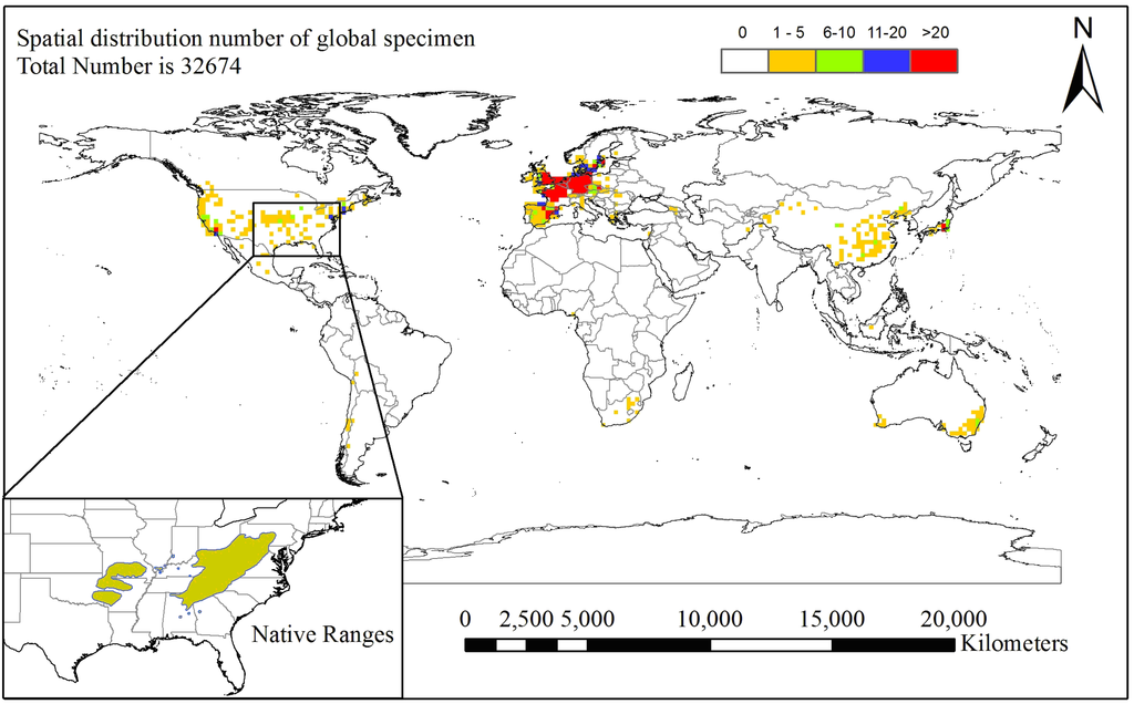
Figure 1.
Global spatial abundance of black locust specimens around the world (the grid cell is 1.5° × 1.5°) and its native range in eastern North America [1]; the total number of specimens is 32,674 (32,434 from Global Biodiversity Information Facility (GBIF) and 240 from Chinese Virtual Herbarium (CVH); the GBIF database query date is 9 May 2014, and the CVH database query date is 10 May 2014.
With the development of computer hardware and Internet speed, the current availability of species and climate information sharing systems has greatly enhanced the field of SDM [19,20,21,22]. These have greatly inspired the use of a variety of algorithms for predicting the potential distribution of species. The performance of various SDM algorithms have been evaluated by numerous comparative studies, suggesting that the appropriate choice is dependent on multiple factors (e.g., sample size, species rarity, size of the species’ geographic range, spatial scale and user preference) [13,23,24]. Because black locust is a wide-ranging species, known to be present at various locations around the world (the distribution data collection process is described in Section 2.1.), maximum entropy modeling was used here to simulate its potential distribution. Maximum entropy modeling uses only presence data as the basis of its predictions, unlike presence/absence models, and is therefore more valuable in regions where collecting absence points has been problematic or completely neglected [25,26]. It has recently been proven to be an effective tool for predicting potential species distributions in a wide variety of research studies [27,28,29].
Climate is considered to be the most important environmental factor influencing the distribution of species and vegetation at a regional and global scale [30,31,32,33]. Therefore, our research has mainly concentrated on investigating the climatically suitable habitat, significant climatic factors, climatic thresholds (niche) and climatic response curves of this species. In this study, species occurrence data with a spatial resolution of 0.5° × 0.5° (approximately 55 km at the Equator; the reason for using this resolution is given in Section 2.1.), together with a system collating 13 climatic indexes (detailed information is given in Section 2.2), were input into a MaxEnt model to simulate the potential distribution area of black locust around the world. The main objectives of the present study were to simulate the ecological niche of black locust, analyze its ecological and geographical distribution and investigate primary climatic factors that determine the potential distribution of this tree around the world. The results could provide theoretical support for top-level design by policy-makers and planners for the introduction, cultivation, planting and invasion control of this species around the world.
2. Material and Methods
2.1. Species Occurrence Data
Global black locust occurrence data were collected from herbarium records in the Global Biodiversity Information Facility database (GBIF) [34] and the Chinese Virtual Herbarium database (CVH) [35]. A total of 32,556 herbarium records were collected from the GBIF database and 319 from the CVH database. Records without coordinates were deleted, and records from small Pacific and Atlantic islands were also deleted, because assigning coarse resolution coordinates (0.5° × 0.5°) to these records may lead to their corresponding climate data being inaccurate. A total of 32,674 specimens (32,434 from GBIF and 240 from CVH) were identified by the coordinates recorded in the database or by coordinates derived from a place name included in the database. The main reason for collating records with a coarse geographic resolution (0.5° × 0.5°) was that there may have been a sampling bias or error at a fine resolution in the GBIF and CVH occurrence records, which would produce models of lower rather than higher quality [21]. Another consideration was the calculation speed of the computer, identified in many previous studies, which was based on a spatial resolution between 50 km × 50 km and 200 km × 200 km [20,21,36]. A total of 1174 grid cells (0.5° × 0.5°) were identified globally as containing black locust (details of the calculation process are given in Section 2.4.). To clearly show the spatial abundance distribution of the 32,674 specimens around the world, the point density function in ArcGIS 9.3 (ESRI, Redlands, CA, USA) was used to draw a 1.5° × 1.5° resolution distribution map of black locust (Figure 1) with its native range in eastern North America based on Little [1].
2.2. Climatic Variables
According to previous studies, there are many variables used to characterize hydrological-thermal climatic niches around the world. For example, 19 BIOCLIM variables were used to define global climatic niches in the WorldClim database [19,37]; three variables (annual biotemperature, potential evapotranspiration and annual precipitation) were used to define global climatic niches in the life zone model [30]; and three variables (warmth index, coldness index and humidity index) were used to represent global climatic niches in Kira’s index system [38]. Three groups of climatic variables are widely used in research on the relationship between species/vegetation and climate, on a regional or global scale. The 19 BIOCLIM variables are widely used in SDM studies, as the data can be easily downloaded from the WorldClim database with no further calculation required [39,40,41]. The five integrated climatic variables (not including annual precipitation) are seldom used in SDM studies, but they can still generally provide considerable power for explaining species distributions [42,43,44,45,46].
In this study, we used the BIOCLIM variables and the five integrated climatic variables based on Holdridge’s life zone model and Kira’s index system. An excess of climatic variables can cause overfitting, so we selected 8 of the 19 BIOCLIM variables. A total of 13 climatic factors were used to define the climatic niches of the world (Table 1), which is sufficient for research on any species at a global scale, including black locust. Baseline climatic layers were downloaded from the WorldClim database with a 10 arc-min spatial resolution, which were generated using thin-plate smoothing splines of latitude, longitude, altitude and monthly temperature and precipitation records from 50-year climate station averages from 1950 to 2000 [19]. Then, these layers were converted to a 0.5° × 0.5° spatial resolution across the globe, and some climatic variables were calculated using the corresponding formulae (Table 1).

Table 1.
Description of 13 climatic factors, corresponding calculated formula and reference.
| Variable | Abbreviation | Unit | Formula and Reference |
|---|---|---|---|
| Annual mean temperature | AMT | °C | - |
| Mean temperature of the warmest month | MTWM | °C | - |
| Mean temperature of the coldest month | MTCM | °C | - |
| Annual range of temperature | ART | °C | Max temperature of warmest month-Min temperature of coldest month |
| Annual precipitation | AP | mm | - |
| Precipitation of wettest month | PWM | mm | - |
| Precipitation of driest month | PDM | mm | - |
| Precipitation of seasonality | PSD | - | Monthly coefficient of variation |
| Annual biotemperature | ABT | °C | ABT = (∑T)/12 (T is 0 < T < 30 °C mean month temperature) [30] |
| Warmth index | WI | °C | WI = ∑(T-5) (T is >5 °C mean month temperature) [38] |
| Coldness index | CI | °C | CI = ∑(T-5) (T is <5 °C mean month temperature) [42] |
| Potential evapotranspiration | PET | mm | PER = 58.93 × ABT/AP (ABT is annual biotemperature, AP is annual precipitation) [30] |
| Humidity index | HI | mm/°C | HI = AP/WI (AP is annual precipitation, WI is the warmth index) [46] |
2.3. Model Selection and Evaluation
In this study, we used the software, MaxEnt (Version 3.0), a machine learning algorithm designed by Phillips et al. [25]. It is written in Java, so it can be used on all modern computing platforms, and is freely available on the Internet at [47]. The main advantage of applying MaxEnt to the modeling of geographical species distributions in comparison with other methods is that it only needs presence data, besides the environmental layers. Furthermore, it is possible to use both categorical and continuous layers. Phillips et al. [25,48] found that MaxEnt outperformed the genetic algorithm for rule set prediction (GARP) [49] on observational data for North American breeding birds and two Neotropical mammals (Bradypus variegatus and Microryzomys minutus). Elith et al. [13] found that MaxEnt was one of the best of 16 different methods for modeling the distributions of 226 species in 6 different regions. Similarly, Wisz et al. [24] found that MaxEnt was one of the best predictors among 12 different models tested.
MaxEnt applies five different feature constraints (linear, quadratic, product, threshold and hinge) to environmental variables, namely “the maximum entropy principle”, to estimate the species distribution probability. This principle can be considered as a constrained optimization problem (where the aim is to maximize a function). The estimated MaxEnt probability distribution (Gibbs distribution) of location (χ) is exponential in a weighted sum of environmental features (f) divided by a scaling constant (Zλ, Equation 1) to ensure that the probability values range from 0 to 1 and sum to 1 [50].
where n is the number of environmental features, λ is the vector of the feature weights, with real values, and Zλ is the normalizing constant that guarantees that the probability distribution sums to one over the area of interest.
MaxEnt provides output data in three formats: raw format (raw values must sum to 1), cumulative format (the value for each cell is equal to the probability of finding the species of interest at that cell plus all other cells with equal or lower probability; values range from 0 to 1) and logistic format (the probability of occurrence is estimated by including environmental variables; values range from 0 to 1) [51]. Raw values are often very small for each data point, thereby making interpretation difficult. The cumulative format is more easily interpreted when projected in a geographic information system, but these projections are not necessarily proportional to the probability of occurrence. The logistic format is currently recommended, because it allows for an easier and potentially more accurate interpretation compared to the other approaches.
MaxEnt modeling can determine the importance of environmental variables using a jackknife test and the regularized gain change during each iteration of the training algorithm. Caution must be used when employing this method, as strong collinearity can influence the results, due to the highly correlated variables. MaxEnt allows the construction of response curves to illustrate the effect of selected variables on the probability of occurrence. These response curves consist of the specific environmental variable as the x-axis and, on the y-axis, the predicted probability of suitable conditions as defined by the logistic output. Upward trends for variables indicate a positive relationship; downward movements represent a negative relationship; and the magnitude of these movements indicates the strength of the relationship [51].
An important part of determining the ability of niche models to predict the distribution of a species is having a measure of fit. The performance of the MaxEnt model is usually evaluated by the threshold-independent receiver operating characteristic (ROC) approach (calculating the area under the ROC curve (AUC) as a measure of prediction success). The ROC curve is a graphical method that represents the relationship between the false-positive fraction (one minus the specificity) and the sensitivity for a range of thresholds. It has a range of 0–1, with a value greater than 0.5 indicating a better-than-random performance event [52]. A rough classification guide is the traditional academic point system [53]: poor (0.5–0.6), fair (0.6–0.7), good (0.7–0.8), very good (0.8–0.9) and excellent (0.9–1.0).
2.4. Experimental Design and Statistical Analysis
First, we plotted all 32,674 black locust specimens’ occurrence records on the world map with a 0.5° × 0.5° spatial resolution. This means that the world map was divided into grid cells (land area with 584,521 cells) with 300 rows and 720 columns. We assumed that a grid cell was suitable for black locust survival, as long as one or more specimens were present in it. Then, a binary grid map (presence/absence map) with a 0.5° × 0.5° spatial resolution was converted into points by using the raster-to-point function in ArcGIS 9.3 (a total of 1174 occurrence points). The latitude and longitude coordinates of each occurrence point (see attachment Supplementary Excel) were stored in an Excel database for MaxEnt model building.
Second, we loaded the latitude and longitude coordinates of the black locust occurrence points into MaxEnt, together with all 13 climatic layers. A ten-fold cross-validation method was used to assess the accuracy of the MaxEnt model predictions. The importance of climatic factors was evaluated by using a jackknife test and the regularized gain change during each iteration of the training algorithm. Otherwise, the default settings were used to run the MaxEnt model. The logistic format of the MaxEnt output was used for mapping habitat suitability. To avoid potential problems due to the effect of strongly correlated factors on the explanation of species response curves, these curves were created by using the MaxEnt model with only the corresponding variable. These curves reflect the dependence of the predicted suitability on the selected variable and reflect the dependency resulting from correlation between the selected variable and other variables.
Finally, the MaxEnt model produced ten species-distribution probability maps based on ten-fold cross-validation. The ten probability maps were then averaged to obtain a habitat suitability map for black locust. Four arbitrary habitat categories were used: the core area (0.6–1.0), the moderately suitable area (0.4–0.6), the marginal area (0.2–0.4) and the unsuitable area (0–0.2), based on the predicted habitat suitability map. The climatic thresholds for each habitat class were analyzed using ArcGIS 9.3.
3. Results
3.1. Current and Potential Distribution of Black Locust
Based on the locations of black locust specimens in the GBIF and CVH databases, the map of the present distribution is shown in Figure 1. Black locust occurs mainly in 35 countries: America, Canada, Mexico, Chile, Bolivia, Argentina (only one record), China, Japan, Afghanistan, Pakistan, Indonesia, Australia, South Africa, Nigeria, Ireland, United Kingdom, Portugal, Spain, France, Germany, Belgium, the Netherlands, Switzerland, Italy, Austria, Czech Republic, Poland, Hungary, Romania, Greece, Georgia, Armenia, Denmark, Norway and Sweden. Large numbers of specimens were collected in North America, Europe and Asia.
The ten probability maps obtained from the ten-fold cross-validation were averaged to obtain a habitat suitability map for black locust (Figure 2). According to the probability values, four habitat categories were defined: the core area (0.6–1.0), the moderately suitable area (0.4–0.6), the marginal area (0.2–0.4) and the unsuitable area (0–0.2). The core suitable areas for black locust are distributed mainly in the eastern United States, Europe, Australia and New Zealand. The moderately-suitable areas mainly included China, Japan, South Africa, Chile and Argentina. In Europe, the core areas are the United Kingdom, Germany, France, the Netherlands, Belgium, Italy and Switzerland. Climatic threshold information for each habitat class is shown in Table 2. It shows the climatic thresholds for the core areas of black locust: a coldness index of −9.8 °C–0 °C, an annual mean temperature of 5.8 °C–14.5 °C, a warmth index of 66 °C–168 °C and an annual precipitation of 508–1867 mm.
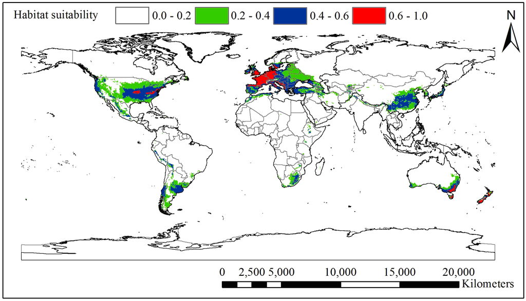
Figure 2.
Global potential distribution area of black locust predicted by the MaxEnt model around the world (the grid cell is 0.5° × 0.5°); the value of climatic suitability is the average of a ten-fold cross-validation. The standard deviation of each grid square is 0–0.11.
Figure 2.
Global potential distribution area of black locust predicted by the MaxEnt model around the world (the grid cell is 0.5° × 0.5°); the value of climatic suitability is the average of a ten-fold cross-validation. The standard deviation of each grid square is 0–0.11.

Table 2.
Climatic threshold of black locust suitable habitat map predicted by the MaxEnt model.
| Climatic Factor | Relative Importance % | Climatic Suitable Habitat Map | |||
|---|---|---|---|---|---|
| Core Area 0.6–1.0 | Moderately Suitable Area 0.4–0.6 | Marginal Area 0.2–0.4 | Unsuitable Area 0–0.2 | ||
| CI | 27.92 | −9.8–0.0 | −26.0–0.0 | −59.7–0.0 | −328.2–0.0 |
| AMT | 22.03 | 5.8–14.5 | 3.9–18.4 | −1.8–22.0 | −26.9–31.3 |
| WI | 15.84 | 66.0–168.0 | 48.7–215.5 | 14.1–258.1 | 0.0–369.9 |
| MTCM | 8.96 | −9.5–5.5 | −15.3–6.3 | −22.1–13.0 | −54.7–25.6 |
| AP | 7.68 | 508.0–1867.0 | 298.0–3199.0 | 34.0–3309.0 | 0.0–8088.0 |
| ABT | 7.13 | 5.9–14.5 | 4.4–18.4 | 1.4–22.0 | 0.0–29.4 |
| PDM | 4.15 | 3.0–93.0 | 1.0–99.0 | 0.0–187.0 | 0.0–492.0 |
| MTWM | 2.15 | 18.0–33.2 | 17.1–39.1 | 11.9–39.4 | −5.9–48.8 |
| PSD | 1.63 | 7.0–101.0 | 6.0–143.0 | 7.0–140.0 | 0.0–261.0 |
| HI | 1.28 | 4.7–19.1 | 2.1–31.2 | 0.2–49.8 | 0.0–100.0 |
| ART | 0.70 | 16.3–40.2 | 16.3–44.2 | 12.4–52.0 | 5.4–72.4 |
| PWM | 0.40 | 52.0–246.0 | 47.0–507.0 | 8.0–749.0 | 0.0–1728.0 |
| PET | 0.13 | 0.2–1.0 | 0.1–2.3 | 0.1–19.4 | 0.0–1508.6 |
Note: The abbreviations of climatic factors and their units can be found in Table 1.
3.2. Model Performance and Importance of Climatic Factors
Ten-fold cross-validation was used to evaluate the accuracy of the MaxEnt model. The accuracy of the resulting model predictions is shown in Figure 3; the MaxEnt model predictions were highly accurate (AUC > 0.9), with a mean AUC of 0.9165 (0.9033–0.9309). The coefficient of variation was only 0.8% among the ten predictions, indicating that the ten-fold cross-validation method does not affect the accuracy of the MaxEnt model simulation.
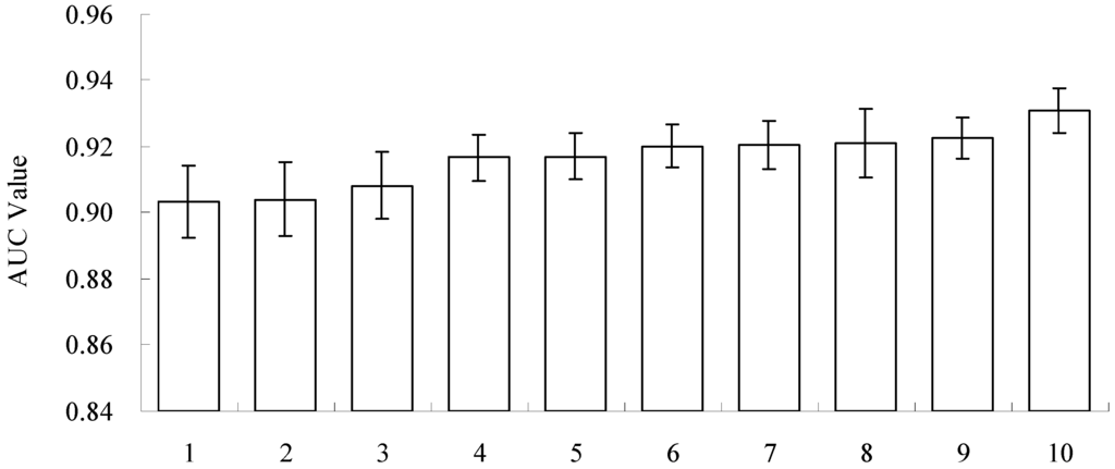
Figure 3.
Areas under the receiver operating characteristic curve (AUC) values of ten-fold cross-validation models (1–10 represent the model code, ascending in order by AUC value; the mean AUC value is 0.9165).
Figure 3.
Areas under the receiver operating characteristic curve (AUC) values of ten-fold cross-validation models (1–10 represent the model code, ascending in order by AUC value; the mean AUC value is 0.9165).

The relative importance of the climatic factors is shown in Figure 4. It is apparent that the coldness index, the annual mean temperature and the warmth index are the most important climatic factors determining the distribution of black locust; these three factors explain 65.79% of the variance, (15.84%–27.92% for each factor), followed by the mean temperature of the coldest month, the annual precipitation and the annual biotemperature, which explain another 23.77% of the variance (7.13%–8.96% for each factor). The remaining seven climatic factors were less important in determining the geographical distribution of black locust (collectively, they explained 10.44% of the variance, 0.13%–4.15% for each factor).
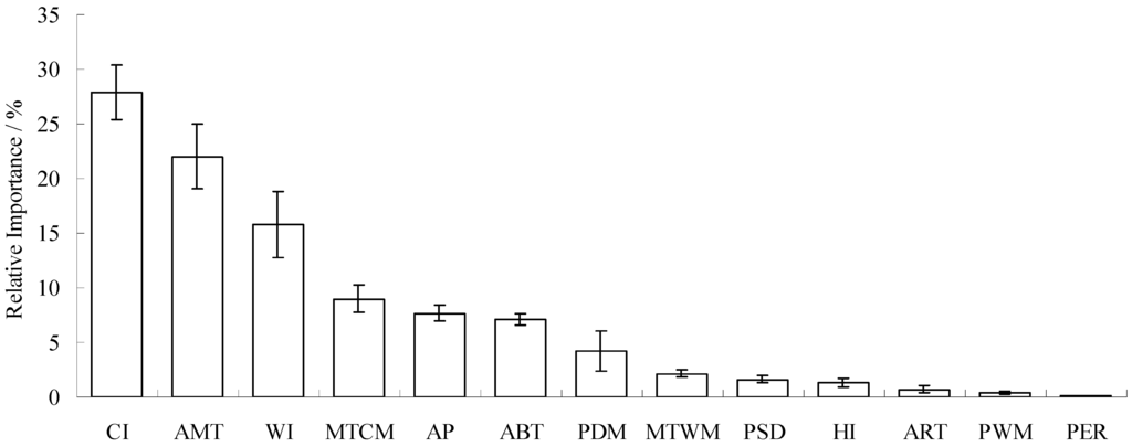
Figure 4.
The relative importance of climatic factors (descending in order). The abbreviations CI, AMT, WI, WTCM, AP, ABT, PDM, MTWM, PSD, HI, ART, PWM and PET can be found in Table 1.
Figure 4.
The relative importance of climatic factors (descending in order). The abbreviations CI, AMT, WI, WTCM, AP, ABT, PDM, MTWM, PSD, HI, ART, PWM and PET can be found in Table 1.

The response curves of black locust under all climatic factors is shown in Figure S1. The first three most important climatic factors (coldness index, annual mean temperature and warmth index) are shown in Figure 5. It is clear that unimodal relationships exist between the habitat suitability value and the annual mean temperature or warmth index, whereas the coldness index shows a linear relationship. The response peak in black locust habitat suitability for the coldness index was at 0 °C; for the annual mean temperature, it was at 9.8 °C; and for the warmth index, it was at 100 °C.

Figure 5.
The response curve of climatic suitability for three dominant climatic factors based on MaxEnt model; (A) Coldness index (CI, °C); (B) annual mean temperature (AMT, °C); (C) warmth index (WI, °C); linear response curve (CI); unimodal response curve (AMT, WI).
Figure 5.
The response curve of climatic suitability for three dominant climatic factors based on MaxEnt model; (A) Coldness index (CI, °C); (B) annual mean temperature (AMT, °C); (C) warmth index (WI, °C); linear response curve (CI); unimodal response curve (AMT, WI).

4. Discussion
4.1. Species Record Database and Species Modeling Tools
The current availability of species-sharing information systems around the world makes it possible to easily study the geographical distribution of plants worldwide [20,21,22]. GBIF is a free and open access biodiversity database that integrates existing worldwide biodiversity data to form a user-oriented global biodiversity service network. CVH is also a free and open access database, which integrates the herbarium data of national natural museums from 14 institutes in China. GBIF and CVH are complementary to each other with little duplication of occurrence records, which makes the occurrence records of CVH a great contribution to GBIF. The old interface of GBIF (which is still available, but not being further developed with new data) [54] includes the capability to quickly generate an SDM niche model (a variant of BIOCLIM rather than MaxEnt; for instructions, see Section 3.1 of Booth [22]). The GBIF niche model output, generated with the 19 BIOCLIM variables, appears to indicate an overly broad climatic suitability (see Supplementary Figure S2) when compared with Figure 2. This may be due to our inclusion of the CVH occurrence records from China, which has improved the SDM niche model’s predictive performance. The new GBIF interface [34] no longer includes the SDM niche model option, so users are forced to perform their own SDM analyses outside of GBIF. GBIF now has so many data points that the providers of the service are concentrating on just storing the data and not providing many integrated analytical tools. Here, we provide a workflow (in Section 2.4) for predicting the potential distribution of a species based on a MaxEnt model, which may be useful for other species. We believe that if every country in the world contributed the data from their national herbaria to the GBIF database, we would be able to make more accurate predictions about our Earth in the near future by using SDM.
At an ecosystem scale, many climate-vegetation models have been used to study the relationship between vegetation and climate, such as Holdridge’s life zone model [30], Kira’s index model [38] and the dynamic vegetation model [55,56]. At a species scale, previous studies have normally used the peak width at half height (PWH) to study the climatic thresholds of species [45,57]. PWH generally assumes that the response of the species to climatic factors is normally distributed. For example, Ni and Song [44] used this method to study the relationship between geographical distribution and climate for Cyclobalanopsis glauca in China. SDM provides another way to study species-climate relationships at a species scale, which does not assume that the response of the species to environmental factors is normally distributed. SDM is widely used, because it can simulate a species’ potential distribution and simultaneously identify significant environmental factors [13,14,25]. For example, Irfan-Ullah et al. [58] predicted the geographical distribution of Aglaia bourdillonii in India, and Li et al. [41] simulated the potential distribution of Quercus wutaishanica in China. This study uses the maximum entropy model, a very popular SDM, to predict the worldwide geographical distribution of black locust. The performance of MaxEnt reached a very high level (a mean AUC value of 0.9165) with a coefficient of variation of only 0.8%, indicating that the MaxEnt model was suitable for simulating the potential distribution of this species around the world. The response curves of black locust to dominant climatic factors show that there is a unimodal response to the annual mean temperature and warmth index and a linear response to the coldness index. The MaxEnt model does not assume that the response of the species distribution to climatic factors is a predefined normal distribution. Therefore, both types of response curve could be detected by the MaxEnt model (Figure 5 and Figure S1).
4.2. Significant Climatic Factors, Geographical Boundary and Potential Distribution Area
In this study, we found that the coldness index, annual mean temperature and warmth index are the most important climatic factors for determining the potential distribution of black locust (with these three factors determining 65.79% of the variance). According to Chuine’s explanation [59] for why phenology drives species distribution, we infer that these three climatic factors may play different roles in the growth process of black locusts. The coldness index (reflecting the extent of harsh climatic conditions during the non-growing season, with a relative contribution of 27.92%) can be interpreted as the cold-climate stress that drives the maturation of fruit later in the growing season, which means that black locusts cannot continue to expand into higher latitudes. The warmth index (reflecting heat conditions during the species growing season, with a relative contribution of 15.84%) can be interpreted as the high thermal climatic conditions that suppress black locust flowering and leafing early in the growing season, such that the tree cannot continue to expand into lower latitudes. The mean annual temperature, with a relative 22.03% contribution, reflects the annual species heat demand during the growing season. Fang and Lechowicz [43] also found that heat-related climatic factors were the limiting factors of the geographical distribution of Fagus spp. around the world, especially the heat conditions during the growing season. Their conclusions were similar to ours.
The core suitable areas in the global potential distribution of black locust are mainly distributed among the eastern United States, Europe, Australia and New Zealand, whereas the moderately suitable areas are mostly in China, Japan, South Africa, Chile and Argentina (Figure 2). These countries are very suitable for afforestation with or introduction of black locust, but we should be aware of the high risk of the invasive potential of this species in these countries. When we compare the difference between the current data available in GBIF and CVH and the potential distribution of black locust (see attachment Figure S3), we could not find any occurrence records in the following 24 countries: Peru, Uruguay, Brazil, Zimbabwe, Kenya, Ethiopia, Morocco, Algeria, New Zealand, Croatia, Bosnia and Herzegovina, Yugoslavia, Albania, Macedonia, Bulgaria, Turkey, Iran, Azerbaijan, Ukraine, Belarus, Lithuania, Latvia, Estonia and Russia, most of which are developing countries. Though we do not know if black locust exists in these countries (due to the lack of web-based open access sharing of data about this species through GBIF from the national herbaria of these countries), we can conclude that this species could be introduced to these countries and may pose a potential threat of invasion there.
4.3. Climatic Threshold and Its Implication
Based on the map of the climatically suitable habitat for this species (Figure 2), we infer that the climatic thresholds of the core area of black locust are a coldness index of −9.8 °C–0 °C, an annual mean temperature of 5.8 °C–14.5 °C, a warmth index of 66 °C–168 °C and annual precipitation of 508–1867 mm. These climatic thresholds may define the most suitable climatic niche, as the occurrence points input into the MaxEnt model come from not only native areas, but also invaded and cultivated areas around the world. Petitpierre et al. [60] reported a large-scale test of climatic niche conservatism for 50 invasive terrestrial plant species from Eurasia, North America and Australia. Their findings reveal that substantial niche shifts are rare in terrestrial plant invaders, providing support for an appropriate use of SDM for the prediction of both biological invasions and responses to climate change. Therefore, we can use the climatic thresholds reported in Table 2 and the response curves in Figure S1 as references to relate to local weather station data to indicate when future invasion control should be initiated or when this species can be used for afforestation, especially on a small geographical scale.
Some studies have reported that the local soil moisture level is an important factor in determining the distribution and growth of black locust at a small scale [61]. Therefore, the use of just climatic factors, on a large scale and with a coarse resolution, to simulate suitable habitat may overestimate the potential distribution of this species. When more types of variables are used, such as soil factors, the niche of the species will be more accurate, and the modeled distributions can be much more credible. Guisan and Thuiller [12] stated that “a gradual distribution observed over a large extent and at coarse resolution is likely to be controlled by climatic regulators, whereas patchy distribution is more likely to result from a patchy distribution of resources, driven by micro-topographic variation or habitat fragmentation”. In their hierarchical modeling framework (see Figure 3 in Guisan and Thuiller [12]), climatic factors were used to determine species ranges on a large scale with coarse resolution, while soil nutriments determined species ranges on a local scale with fine resolution. We recommend further research on the hierarchical prediction of black locust distribution with the integration of more types of environmental factors, at the national or regional scale with fine resolution in the climatically suitable countries identified here. Our research has mainly concentrated on the habitat that currently has the potential to be climatically suitable and the climatic niche of this species on a global scale with coarse resolution. The predictive map of black locust distribution, the climatic thresholds and the species response curves can provide global perspective guidelines and valuable information for policymakers and planners of introductions, planting and invasion control of this species around the world.
5. Conclusions
Black locust is native to eastern North America, and has already spread widely all over the world by transplantation and cultivation in recent 300 years. On the one hand, black locust is a tree species of high ecological and economic value (as a pioneer species, a nurse species, an ornamental species, a feed species, etc.). On the other hand, it is also a serious invasive species in some parts of the world (such as Britain, Germany, France, Japan, etc.). This study comprehensively integrate the global herbarium data of black locust (from Global Biodiversity Information Facility and Chinese Virtual Herbarium) and the world climate system (BIOCLIM system, Holdridge life zone system, and Kira’s index system) using maximum entropy modeling to research the climatic suitable habitat, significant climatic factors, climatic thresholds (niche) and climatic response curves of this species at global scale with coarse resolution. Realized distribution area and potential distribution area are compared for figuring out the suitable area for invasive control or afforestation of this species. The climatic thresholds and response curves could be used as references to relate to the data of local weather station to indicate when future invasion control should be initiated or when this species can be used for afforestation, especially on a small geographical scale. In addition, the climate system (in Section 2.2) and the simulating workflow (in Section 2.4) in this study could be useful when the global potential distribution of other species is predicted.
Acknowledgments
We are very grateful to two anonymous reviewers for their valuable suggestions, which significantly improved the manuscript. We thank Yang Cao for his help with improving our language expression. The project was supported financially by the National Nature Science Foundation of China (No. 31300407), the Specialized Research Fund for the Doctoral Program of Higher Education (No. 20130204120028) and the Institute of Soil and Water Conservation, CAS&MWR (A315021441).
Author Contributions
All authors contributed extensively to this work. Conceived of and designed the experiments: Guoqing Li, Guanghua Xu, Ke Guo and Sheng Du. Collected and analyzed the data: Guoqing Li and Guanghua Xu. Wrote the paper: Guoqing Li.
Supplementary

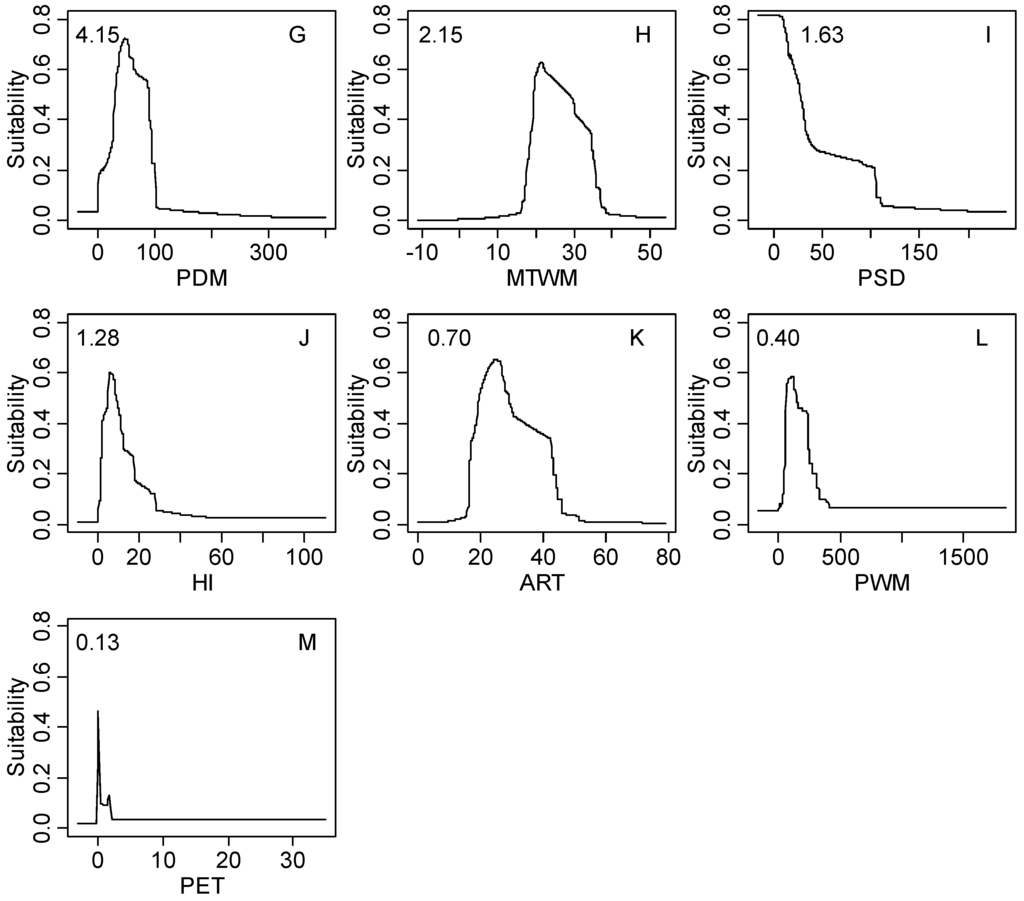
Figure S1.
The response curves of climatic habitat suitability values for all climatic factors based on the MaxEnt model decreasing in order based on their relative importance (shown in the upper-left corner of each subplot); (A) Coldness index (CI, °C); (B) annual mean temperature (AMT, °C); (C) warmth index (WI, °C); (D) mean temperature of the coldest month (MTCM, °C); (E) annual precipitation (AP, mm); (F) annual biotemperature (ABT, °C); (G) precipitation of driest month (PDM, mm); (H) mean temperature of the warmest month (MTWM, °C); (I) precipitation of seasonality (PSD, mm); (J) humidity index (HI, mm/°C); (K) annual range of temperature (ART, °C); (L) precipitation of wettest month (PWM); (M) potential evapotranspiration (PET, mm).
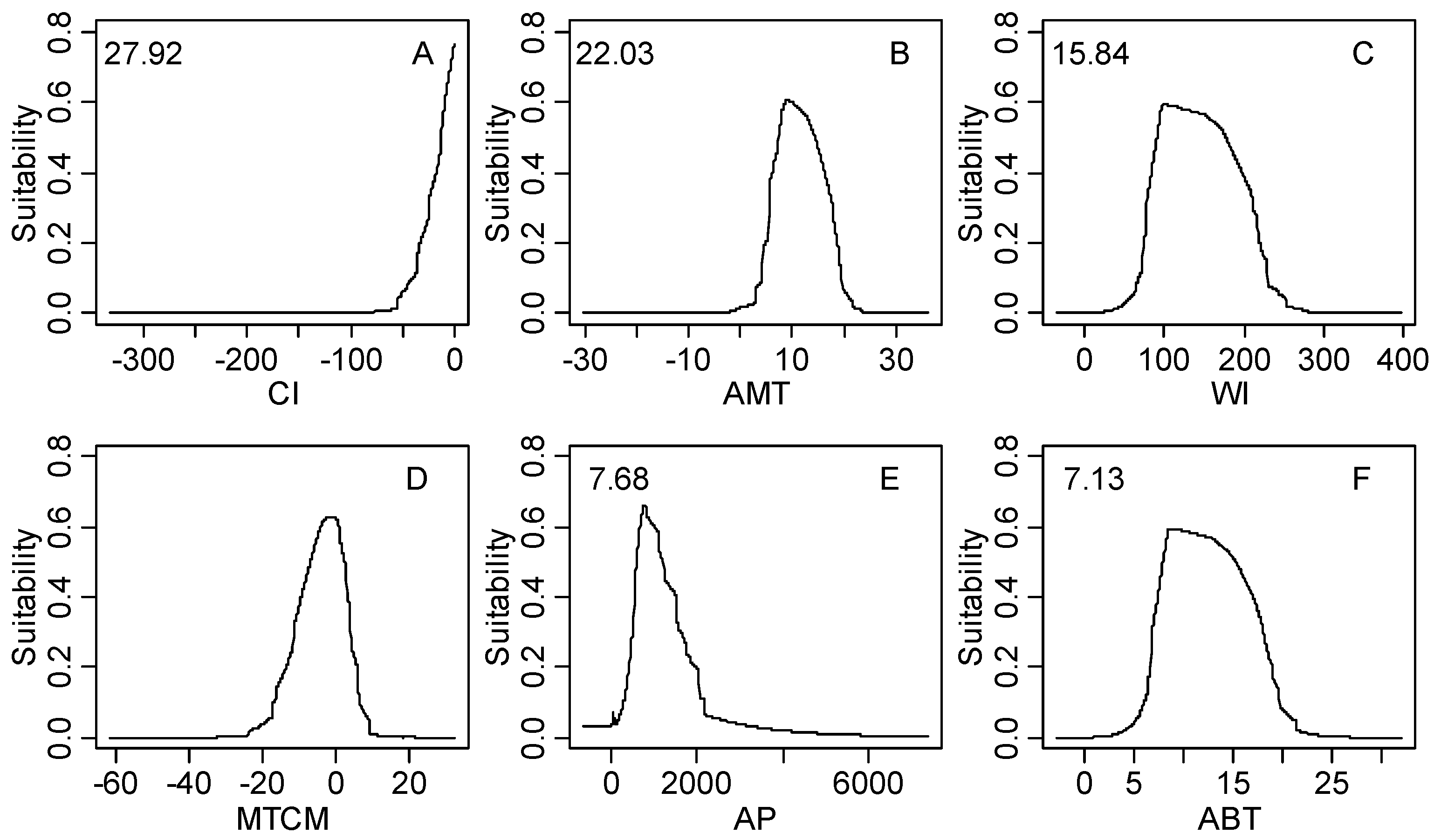


Figure S2.
Niche model generated within the old GBIF interface using 19 BIOCLIM factors with 31,873 GBIF records; the climatic suitability appears much too broad.
Figure S2.
Niche model generated within the old GBIF interface using 19 BIOCLIM factors with 31,873 GBIF records; the climatic suitability appears much too broad.
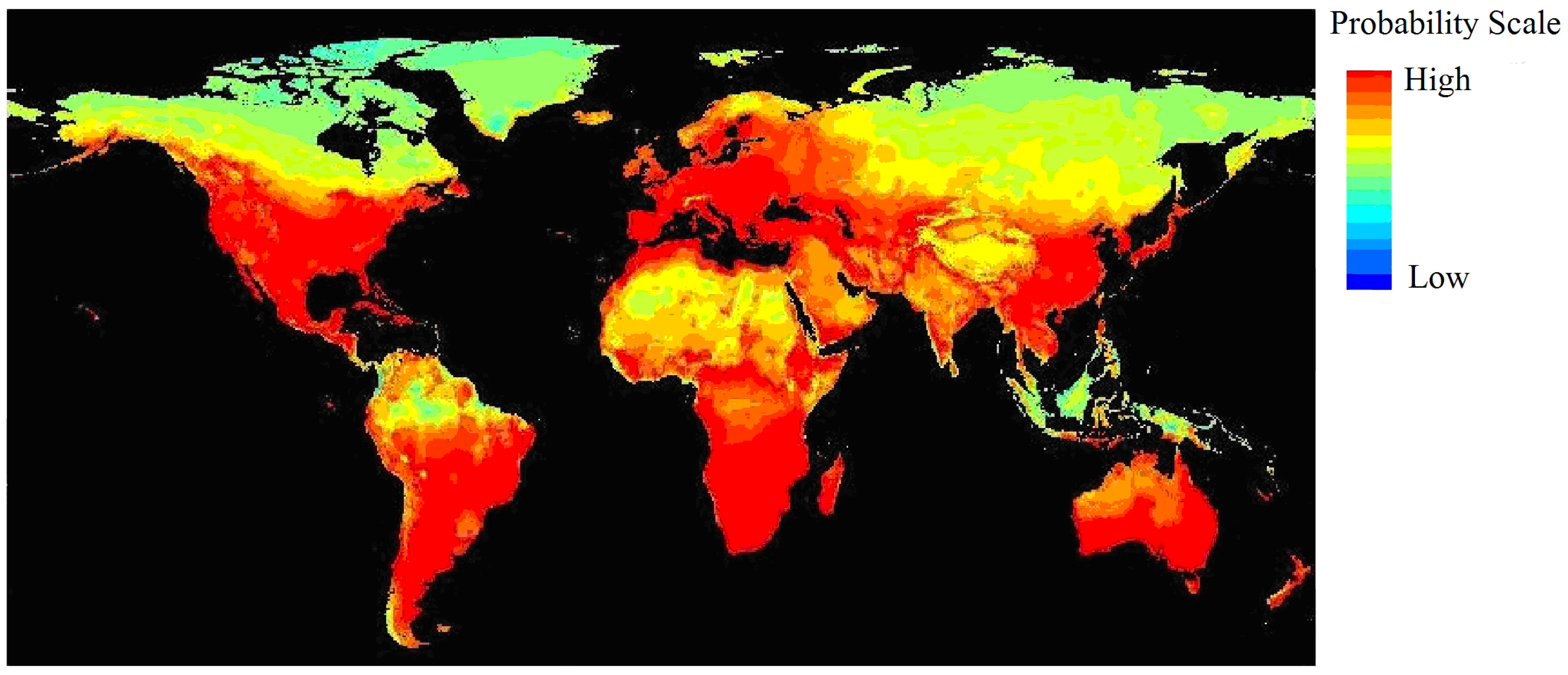
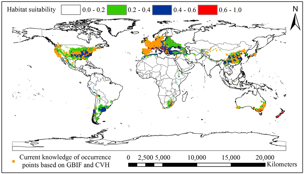
Figure S3.
The difference between the current distribution knowledge of GBIF and CVH and the potential distribution of black locust. No occurrence records were found in the following 24 countries: Peru, Uruguay, Brazil, Zimbabwe, Kenya, Ethiopia, Morocco, Algeria, New Zealand, Croatia, Bosnia and Herzegovina, Yugoslavia, Albania, Macedonia, Bulgaria, Turkey, Iran, Azerbaijan, Ukraine, Belarus, Lithuania, Latvia, Estonia and Russia, most of which are developing countries.

Conflicts of Interest
The authors declare no conflict of interest.
References
- Little, E.L. Atlas of United States trees. In Conifers and Important Hardwoods; US Department of Agriculture, Forest Service: Washington, DC, USA, 1971. [Google Scholar]
- Delectis Florae Reipublicae Popularis Sinicae Agendae Academiae Sinicae Edita. In Flora Reipublicae Popularis Sinicae; Science Press: Beijing, China, 1994; p. 228.
- Huntley, J.C. Robinia pseudoacacia L. Black locust. In Silvics of North America; Hardwoods, Agriculture Handbook, No. 654.; Burns, R.M., Honkala, B.H., Eds.; USDA Forest Service: Washington, DC, USA, 1990; pp. 755–761. [Google Scholar]
- Keresztesi, B. The black locust. Unasylva 1980, 32, 23–33. [Google Scholar]
- Cheeke, P.R. Black locust forage as an animal foodstuff. In Proceedings of the International Conference on Black Locust: Biology, Culture, & Utilization; Hanover, J.W., Miller, K., Plesko, S., Eds.; Department of Forestry, Michigan State University: East Lansing, MI, USA, 1992; pp. 252–258. [Google Scholar]
- Bridgen, M.R. Plantation silviculture of black locust. In Proceedings of the International Conference on Black Locust: Biology, Culture, & Utilization; Hanover, J.W., Miller, K., Plesko, S., Eds.; Department of Forestry, Michigan State University: East Lansing, MI, USA, 1992; pp. 21–32. [Google Scholar]
- Gupta, R.K. Multipurpose Trees for Agroforestry and Wasteland Utilisation; Oxford & IBH Publishing Co.: New Delhi, India, 1993. [Google Scholar]
- Haysom, K.A.; Murphy, S.T. The Status of Invasiveness of Forest Tree Species Outside Their Natural Habitat: A Global Review and Discussion Paper; Forest Health and Biosecurity Working Paper FBS/3E; FAO: Rome, Italy, 2003. [Google Scholar]
- Richardson, D.M.; Rejmanek, M. Trees and shrubs as invasive alien species—A global review. Divers. Distrib. 2011, 17, 788–809. [Google Scholar] [CrossRef]
- Randall, R.P. A Global Compendium of Weeds, 2nd ed.Department of Agriculture and Food: Perth, West Australia, Australia, 2012.
- Cierjacks, A.; Kowarik, I.; Joshi, J.; Hempel, S.; Ristow, M.; Vonderlippe, M.; Weber, E. Biological flora of the British Isles: Robinia pseudoacacia. J. Ecol. 2013, 101, 1623–1640. [Google Scholar] [CrossRef]
- Guisan, A.; Thuiller, W. Predicting species distribution: Offering more than simple habitat models. Ecol. Lett. 2005, 8, 993–1009. [Google Scholar] [CrossRef]
- Elith, J.; Graham, C.H.; Anderson, R.P.; Dudik, M.; Ferrier, S.; Guisan, A.; Hijmans, R.J.; Huettman, F.; Leathwick, J.R.; Lehmann, A.; et al. Nevel methods improve prediction of species’s distribution from occurrence data. Ecography 2006, 29, 129–151. [Google Scholar] [CrossRef]
- Franklin, J. Mapping Species Distributions: Spatial Interence and Prediction; Cambridge University Press: Cambridge, UK, 2009. [Google Scholar]
- Booth, T.H.; Nix, H.A.; Busby, J.R.; Hutchinson, M.F. BIOCLIM: The first species distribution modelling package, its early applications and relevance to most current MAXENT studies. Divers. Distrib. 2014, 20, 1–9. [Google Scholar] [CrossRef]
- Booth, T.H.; Nix, H.A.; Hutchinson, M.F.; Jovanovic, T. Niche analysis and tree species introduction. For. Ecol. Manag. 1988, 23, 47–59. [Google Scholar] [CrossRef]
- Hutchinson, G.E. Concluding remarks. Cold Spring Harb. Symp. Quant. Biol. 1957, 22, 415–427. [Google Scholar] [CrossRef]
- Peterson, A.T.; Soberon, J.; Pearson, R.G.; Andersen, R.P.; Martinez-Meyer, E.; Nakamura, M.; Araujo, M.B. Ecological Niches and Geographic Distributions; Monographsin Population Biology No. 49; Princeton University Press: Princeton, NJ, USA, 2011. [Google Scholar]
- Hijmans, R.J.; Cameron, S.E.; Parra, J.L.; Jones, P.G.; Jarvis, A. Very high resolution interpolated climate surfaces for global land areas. Int. J. Climat. 2005, 25, 1965–1978. [Google Scholar] [CrossRef]
- Jetz, W.; McPherson, J.M.; Guralnick, R.P. Integrating biodiversity distribution knowledge: Toward a global map of life. Trends Ecol. Evol. 2012, 27, 151–159. [Google Scholar] [CrossRef] [PubMed]
- Beck, J.; Ballesteros-Mejia, L.; Nagel, P.; Kitching, I.J. Online solutions and the “Wallacean shortfall”: What does GBIF contribute to our knowledge of species’ ranges? Divers. Distrib. 2013, 19, 1043–1050. [Google Scholar] [CrossRef]
- Booth, T.H. Using biodiversity databases to verify and improve descriptions of tree species climatic requirements. For. Ecol. Manag. 2014, 315, 95–102. [Google Scholar] [CrossRef]
- Tsoar, A.; Allouche, O.; Steinitz, O.; Rotem, D.; Kadmon, R. A comparative evaluation of presence-only methods for modeling species distribution. Divers. Distrib. 2007, 13, 397–405. [Google Scholar] [CrossRef]
- Wisz, M.S.; Hijmans, R.J.; Li, J.; Peterson, A.T.; Graham, C.H.; Guisan, A.; Group, N.P.S.D.W. Effects of sample size on the performance of species distribution models. Divers. Distrib. 2008, 14, 763–773. [Google Scholar] [CrossRef]
- Phillips, S.J.; Anderson, R.P.; Schapire, R.E. Maximum entropy modeling of species geographic distributions. Ecol. Model. 2006, 190, 231–259. [Google Scholar] [CrossRef]
- Phillips, S.J.; Dudik, M.; Elith, J.; Graham, C.H.; Lehmann, A.; Leathwick, J.; Ferrier, S. Sample selection bias and presence-only distribution models: Implications for background and pseudo-absence data. Ecol. Appl. 2009, 19, 181–197. [Google Scholar] [CrossRef] [PubMed]
- Slater, H.; Michael, E. Predicting the current and future potential distributions of Lymphatic filariasis in africa using maximum entropy ecological niche modelling. PLoS One 2012, 7, e32202. [Google Scholar] [CrossRef]
- Yin, X.J.; Zhou, G.S.; Sui, X.H.; He, Q.J.; Li, R.P. Dominant climatic factors of Quercus mongolica geographical distribution and their thresholds. Acta Ecol. Sin. 2013, 33, 103–109. [Google Scholar] [CrossRef]
- Merow, C.; Smith, M.J.; Silander, J.A. A practical guide to MaxEnt for modeling species’ distributions: What it does, and why inputs and settings matter. Ecography 2013, 36, 1058–1069. [Google Scholar] [CrossRef]
- Holdridge, L.R. Determination of world plant formations from simple climatic data. Science 1947, 105, 367–368. [Google Scholar] [CrossRef] [PubMed]
- Woodward, F.I. Climate and Plant Distribution; Cambridge University Press: Cambridge, UK, 1987. [Google Scholar]
- Pearson, R.G.; Dawson, T.P. Predicting the impacts of climate change on the distribution of species: Are bioclimate envelope models useful? Glob. Ecol. Biogeogr. 2003, 12, 361–371. [Google Scholar] [CrossRef]
- Guisan, A.; Tingley, R.; Baumgartner, J.B.; Naujokaitis-Lewis, I.; Sutcliffe, P.R.; Tulloch, A.I.T.; Regan, T.J.; Brotons, L.; McDonald-Madden, E.; Mantyka-Pringle, C.; et al. Predicting species distributions for conservation decisions. Ecol. Lett. 2013, 16, 1424–1435. [Google Scholar] [CrossRef]
- Global Biodiversity Information Facility. Available online: http://www.gbif.org/ (accessed on 9 May 2014).
- Chinese Virtual Herbarium. Available online: http://www.cvh.org.cn/ (accessed on 10 May 2014).
- Ballesteros-Mejia, L.; Kitching, I.J.; Jetz, W.; Nagel, P.; Beck, J. Mapping the biodiversity of tropical insects: Species richness and inventory completeness of African sphingid moths. Glob. Ecol. Biogeogr. 2013, 22, 586–595. [Google Scholar] [CrossRef]
- WorldClim—Global Climate Data. Available online: http://www.worldclim.org/ (accessed on 10 May 2014).
- Kira, T. A New Classification of Climate in Eastern Asia as the Basis for Agricultural Geography; Horticultural Institute, Kyoto University: Kyoto, Japan, 1945. [Google Scholar]
- Acosta, L.E. Distribution of Geraeocormobius sylvarum (Opiliones, Gonyleptidae): Range modeling based on bioclimatic variables. J. Arachnol. 2008, 36, 574–582. [Google Scholar] [CrossRef]
- Livshultz, T.; Mead, J.V.; Goyder, D.J.; Brannin, M. Climate niches of milkweeds with plesiomorphic traits (Secamonoideae; Apocynaceae) and the milkweed sister group link ancient African climates and floral evolution. Am. J. Bot. 2011, 98, 1966–1977. [Google Scholar] [CrossRef] [PubMed]
- Li, G.Q.; Liu, C.C.; Liu, Y.G.; Yang, J.; Zhang, X.S.; Guo, K. Effects of climate, disturbance and soil factors on the potential distribution of liaotung oak (Quercus wutaishanica Mayr) in China. Ecol. Res. 2012, 27, 427–436. [Google Scholar] [CrossRef]
- Kira, T. On the altitudinal arrangement of climatic zones in Japan. Kanchi-Nougaku 1948, 2, 143–173. [Google Scholar]
- Fang, J.Y.; Lechowicz, M.J. Climatic limits for the present distribution of beech (Fagus L.) species in the world. J. Biogeogr. 2006, 33, 1804–1819. [Google Scholar] [CrossRef]
- Ni, J.; Song, Y.C. Relationships between geographical distribution of Cyclobalanopsis glauca and climate in China. Acta Bot. Sin. 1997, 39, 451–460. [Google Scholar]
- Yim, Y.J. Distribution of forest vegetation and climate in the Korean Peninsula. III Distribution of tree species along the thermal gradient. Jpn. J. Ecol. 1977, 27, 269–278. [Google Scholar]
- Xu, W.D. Kira’s temperature indices and their application in the study of vegetation. Chin. J. Ecol. 1985, 3, 35–39. [Google Scholar]
- Maxent Software for Species Habitat Modeling. Available online: http://www.cs.princeton.edu/~schapire/maxent/ (accessed on 10 May 2014).
- Phillips, S.J.; Dudik, M.; Schapire, R.E. A maximum entropy approach to species distribution modeling. In Proceedings of the Twenty-First International Conference on Machine Learning, South Banff, Alberta, Canada, 4–8 July 2004; pp. 655–662.
- Stockwell, D.; Peters, D. The GARP modelling system: Problems and solutions to automated spatial prediction. Int. J. Geogr. Inf. Sci. 1999, 13, 143–158. [Google Scholar] [CrossRef]
- Yost, A.C.; Petersen, S.L.; Gregg, M.; Miller, R. Predictive modeling and mapping sage grouse (Centrocercus urophasianus) nesting habitat using Maximum Entropy and a long-term dataset from Southern Oregon. Ecol. Inform. 2008, 3, 375–386. [Google Scholar] [CrossRef]
- Baldwin, R.A. Use of maximum entropy modeling in wildlife research. Entropy 2009, 11, 854–866. [Google Scholar] [CrossRef]
- Fielding, A.H.; Bell, J.F. A review of methods for the assessment of prediction errors in conservation presence/absence models. Envir. Conser. 1997, 24, 38–49. [Google Scholar] [CrossRef]
- Swets, J. Measuring the accuracy of diagnostic systems. Science 1988, 240, 1285–1293. [Google Scholar] [CrossRef] [PubMed]
- Old Interface of GBIF. Available online: http://data.gbif.org/ (accessed on 10 May 2014).
- Prentice, I.C.; Cramer, W.; Harrison, S.P.; Leemans, R.; Monserud, R.A.; Solomon, A.M. A global biome model based on plant physiology and dominance, soil properties and climate. J. Biogeogr. 1992, 19, 117–134. [Google Scholar] [CrossRef]
- Peng, C.H. From static biogeographical model to dynamic global vegetation model: A global perspective on modelling vegetation dynamics. Ecol. Model. 2000, 135, 33–54. [Google Scholar] [CrossRef]
- Hong, B.G.; Li, S.Z. The preliminary study of the correlations between the distribution of main everygreen broad-leaf tree species in Jiangsu and climates. Acta Ecol. Sin. 1981, 1, 101–111. [Google Scholar]
- Irfan-Ullah, M.; Amarnath, G.; Murthy, M.S.R.; Peterson, A.T. Mapping the geographic distribution of Aglaia bourdillonii gamble (Meliaceae), an endemic and threatened plant, using ecological niche modeling. Biodivers. Conserv. 2007, 16, 1917–1925. [Google Scholar] [CrossRef]
- Chuine, I. Why does phenology drive species distribution? Philos. Trans. R. Soc. B 2010, 365, 3149–3160. [Google Scholar] [CrossRef]
- Petitpierre, B.; Kueffer, C.; Broennimann, O.; Randin, C.; Daehler, C.; Guisan, A. Climatic niche shifts are rare among terrestrial plant invaders. Science 2012, 335, 1344–1348. [Google Scholar] [CrossRef] [PubMed]
- Wang, M.C.; Wang, J.X.; Shi, Q.H.; Zhang, J.S. Photosynthesis and water use efficiency of platycladus orientalis and Robinia pseudoacacia saplings under steady soil water stress during different stages of their annual growth period. J. Integr. Plant Biol. 2007, 49, 1470–1477. [Google Scholar] [CrossRef]
© 2014 by the authors; licensee MDPI, Basel, Switzerland. This article is an open access article distributed under the terms and conditions of the Creative Commons Attribution license (http://creativecommons.org/licenses/by/4.0/).
