Article

Acoustic Velocity—Wood Fiber Attribute Relationships for Jack Pine Logs and Their Potential Utility

Canadian Wood Fiber Centre, Canadian Forest Service, Natural Resources Canada, Sault Ste. Marie, ON P6A 2E5, Canada
Forests 2018, 9(12), 749; https://doi.org/10.3390/f9120749
Submission received: 18 October 2018 / Revised: 15 November 2018 / Accepted: 23 November 2018 / Published: 30 November 2018
(This article belongs to the Special Issue Wood Properties and Processing)

Abstract

:
This study presents an acoustic-based predictive modeling framework for estimating a suite of wood fiber attributes within jack pine (Pinus banksiana Lamb.) logs for informing in-forest log-segregation decision-making. Specifically, the relationships between acoustic velocity (longitudinal stress wave velocity; vl) and the dynamic modulus of elasticity (me), wood density (wd), microfibril angle (ma), tracheid wall thickness (wt), tracheid radial and tangential diameters (dr and dt, respectively), fiber coarseness (co), and specific surface area (sa), were parameterized deploying hierarchical mixed-effects model specifications and subsequently evaluated on their resultant goodness-of-fit, lack-of-fit, and predictive precision. Procedurally, the data acquisition phase involved: (1) randomly selecting 61 semi-mature sample trees within ten variable-sized plots established in unthinned and thinned compartments of four natural-origin stands situated in the central portion the Canadian Boreal Forest Region; (2) felling and sectioning each sample tree into four equal-length logs and obtaining twice-replicate vl measurements at the bottom and top cross-sectional faces of each log (n = 4) from which a log-specific mean vl value was calculated; and (3) sectioning each log at its midpoint and obtaining a cross-sectional sample disk from which a 2 × 2 cm bark-to-pith radial xylem sample was extracted and subsequently processed via SilviScan-3 to derive annual-ring-specific attribute values. The analytical phase involved: (1) stratifying the resultant attribute—acoustic velocity observational pairs for the 243 sample logs into approximately equal-sized calibration and validation data subsets; (2) parameterizing the attribute—acoustic relationships employing mixed-effects hierarchical linear regression specifications using the calibration data subset; and (3) evaluating the resultant models using the validation data subset via the deployment of suite of statistical-based metrics pertinent to the evaluation of the underlying assumptions and predictive performance. The results indicated that apart from tracheid diameters (dr and dt), the regression models were significant (p ≤ 0.05) and unbiased predictors which adhered to the underlying parameterization assumptions. However, the relationships varied widely in terms of explanatory power (index-of-fit ranking: wt (0.53) > me > sa > co > wd >> ma (0.08)) and predictive ability (sa > wt > wd > co >> me >>> ma). Likewise, based on simulations where an acoustic-based wd estimate is used as a surrogate measure for a Silviscan-equivalent value for a newly sampled log, predictive ability also varied by attribute: 95% of all future predictions for sa, wt, co, me, and ma would be within ±12%, ±14%, ±15%, ±27%, and ±55% and of the true values, respectively. Both the limitations and potential utility of these predictive relationships for use in log-segregation decision-making, are discussed. Future research initiatives, consisting of identifying and controlling extraneous sources of variation on acoustic velocity and establishing attribute-specific end-product-based design specifications, would be conducive to advancing the acoustic approach in boreal forest management.

1. Introduction

The Canadian forest sector has been increasingly embracing an aspirational trivariate management proposition for which the goal is to maximize end-product value while simultaneously realizing volumetric yield and ecological sustainability objectives (sensu [1,2]). Tangential to this transformative shift is the increased apprehension regarding the quality and associated end-product potential of the increasing wood volumes harvested from more intensely managed second-growth forests [3]. Among the many prerequisites required for realizing this goal and addressing knowledge gaps in second-growth fiber quality, is the provision of enhanced in-forest intelligence in regards to the forecasting of end-product potential at the time of harvest or immediately afterwards (n., in-forest generically refers to all forest operations conducted or decisions made before mill-processing commences inclusive of operational felling areas, landings and log sorting yards).
End-product forecasts can be used to inform and optimize log-segregation, allocation and merchandizing decision-making thus contributing to the potential realization of the value maximization objective [4,5,6]. More precisely, the end-product potential of the logs extracted from the main stem of individual coniferous trees is a function of (1) external morphological stem features (e.g., diameter, height, taper, sweep, crook, and eccentricity), and (2) internal anatomical characteristics (e.g., microfibril angle, tracheid wall thickness, tracheid radial and tangential diameters) and associated physical properties (e.g., modulus of elasticity, wood density, fiber coarseness and specific surface area) of the xylem tissue. Various performance measures which are used to define and classify the overall type and grade of derived products have been shown to be explicitly linked to these internal fiber-based attributes. Although only stiffness and wood density measures are currently used in machine stress grading systems for solid wood products (e.g., dimensional lumber [7]), microfibril angle, tracheid cell wall thickness, radial and tangential tracheid diameters, fiber coarseness and specific surface area, are also important determinates of end-product quantity and quality [8] (sensu Table 1). Thus, as the fiber supply increases in diversity with the arrival of wood from density manipulated forests (e.g., pre-commercially and/or commercially thinned natural-origin stands, and plantations) combined with increasing pressures to find economic efficiencies within the upper portion of the forest products supply chain, provision of explicit information on these additional attributes may become consequential.
Attribute determination for use in forecasting end-product potential deploying destructive sampling approaches can be logistically challenging, time consuming and expensive (e.g., in-forest extracting of 12 mm diameter xylem cores followed by Silviscan-based laboratory processing and testing). Conversely, non-destructive sampling methods in which attributes can be estimated indirectly through their relationship with acoustic velocity has been shown to be viable alternative [9,10,11,12]. More specifically, in-forest acoustic-based sampling tools provide forest practitioners with an ability to estimate the dynamic modulus of elasticity within harvested logs and standing trees. The dynamic modulus of elasticity is a wood stiffness measure that is used as a surrogate measure of its static counterpart (static modulus of elasticity). This latter static measure is commonly employed along with maximum knot size, sweep and physical dimensions, to categorize solid wood products into specific grade classes [7,9,13]. Thus, the ability to forecast one of the key underlying determinates of end-product potential within the forest at the time of harvest or soon after, has important utility in terms of informing segregation, allocation and merchandizing decision-making [6].
Mathematically, as derived from engineering principles, the dynamic modulus of elasticity (MOEdyn denoted m e in this study; GPa) of a log can be expressed as a function of the density-weighted velocity of a longitudinal stress wave (vl; km/s) that propagates through the xylem tissue upon its generation arising from a mechanically induced impact on one of the open cross-sectional log faces (Equation (1) and denoted the primary relationship herewith; [12]).
m e = f ( w d v l 2 )
where w d is the green (fresh) wood density (kg/m3) of the log’s xylem tissue. The dynamic modulus of elasticity has also been shown to be correlated with other attributes underlying end-product potential [14,15,16].
More specifically, based on extracted clear xylem samples obtained from black spruce (Picea mariana (Mill) B.S.P.), red pine (Pinus resinosa Ait.) and jack pine (Pinus banksiana Lamb.) trees growing in the central North America, Silviscan-derived estimates of wood density (oven-dried wood density denoted w d in this study; kg/m3), microfibril angle (MFA denoted m a in this study; °), tracheid cell wall thickness ( w t ; µm), radial ( d r ; µm) and tangential ( d t ; µm) tracheid diameters, fiber coarseness ( c o ; µg/m) and specific surface area ( s a ; m2/kg), have been shown to be correlated with the dynamic modulus of elasticity (Table 2). Statistically significant (p ≤ 0.05) (1) directly proportional relationships between me and wd, wt and co ( m e w d , w t , c o ) , and (2) indirectly proportional relationships between me and ma, dr, dt and sa ( m e m a 1 , d r 1 , d t 1 , s a 1 ) , have been established for these species (Table 2). Supporting correlative evidence has also been reported for non-boreal conifers. For example, a directly proportional correlative relationship between me and wood density (r = 0.75) and an inversely proportional relationship between me and ma (r = −0.83) has been reported for Silviscan-derived attribute estimates obtained from clear wood samples extracted from 76 radiata pine (Pinus radiata D. Don.) boards [13]. Based on this collective correlative evidence, an empirical-based expansion of the acoustic-based inferential framework was proposed for boreal conifer logs [15], as summarized in Table 2. Since wood density is also one of the principal end-product determinates (sensu Table 1) and analytically required for acoustic-based attribute predictions (e.g., Equation (1); Table 2), a simplified directly proportional relationship between acoustic velocity and wood density was included within this framework (i.e., w d v l 2 ). Collectively, this expanded acoustic inferential framework represents a more encompassing analytical platform for forecasting commercially relevant wood quality attributes than previous univariate approaches solely based on the primary relationship (Equation (1)).
Although these statistical-based secondary relationships lack the causal underpinnings of the primary relationship (sensu [17]), the empirical results to date have been supportive. Specifically, applying this analytical framework to red pine logs, revealed that statistically viable acoustic-based relationships could be established for five of the eight attributes examined (me, wd, wt, co and sa) [15]. However, the applicability of this expanded framework of acoustic-based wood attribute relationships to other intensely managed softwood species is largely unknown. Furthermore, even the most fundamental acoustic velocity—attribute relationship (Equation (1)) has yet to be parameterized for most of the commercially important Canadian boreal conifers (e.g., an “acoustic velocity” keyword search for articles published within Canada’s primary applied journal (Forestry Chronicle) was unsuccessful in identifying previous research in this field). Conversely, other forest regions, such as New Zealand, United States of America, Australia, Europe, and Asia, have adapted this acoustic-based innovation pathway in order improve segregation decision-making (e.g., [18,19]). Hence, the evaluation of the acoustic approach and the provision of prediction equations for the estimating a suite of key attributes underlying end-product potential for jack pine, could contribute to addressing this innovation void. Principally, by providing the forest practitioner with the prerequisite prediction equations, in-forest segregation decision-making could be improved and potentially yield overall efficiency gains within the upper portion of the jack pine forest products supply chain. Consequently, the objective of this study was to investigate the empirical applicability of the expanded acoustic-based inferential framework by examining the nature, strength and predictability of the relationships between acoustic velocity and the dynamic modulus of elasticity, wood density, microfibril angle, tracheid cell wall thickness, radial and tangential tracheid diameters, fiber coarseness and specific surface area, specifically for jack pine.

2. Materials and Methods

2.1. Sample Stands, Plot Establishment and Sample Tree Selection

Two geographically separated jack pine thinning experiments that were previously established in northeastern (denoted the Sewell site) and northcentral (denoted the Tyrol site) regions of Ontario, were selected for sampling. The experimental treatments were representative of the crop planning strategy historically followed in Ontario for this species. Specifically, allowing jack pine to naturally regenerate following a stand-replacing disturbance and if sufficiently successful in terms of stocking levels and free-to-grow status, (1) implementing precommercial thinning in order to moderate overall site occupancy and encourage individual tree growth thereby reducing the time-to-operability status in order to mitigate the effects of projected wood supply deficits, or (2) implementing a temporal sequence of thinning treatments (precommercial and commercial thinning) in order to optimize site occupancy and maximize end-product potentials throughout the rotation [20].
At the Sewell site, sample trees were selected within 6 sample plots that were established in 3 fire-origin jack pine stands (2 plots/stand). These approximately 53-year-old stands were situated on sites of medium-to-good quality (mean site index of 18 m at a breast-height age of 50 [21]) and geographically located within Forest Section B.7—Missinaibi-Cabonga of the Canadian Boreal Forest Region [22]. The soils and topography were characterized as deep (>1 m) coarse-to-medium textured sandy types situated on gently undulating terrain. Silviculturally, the stands were subjected to 1 of 3 density manipulation treatments yielding 3 unique crop plans: (1) natural stand development with no density management (unthinned); (2) precommercial thinned (PCT) at age 11 (1971); and (3) PCT at age 11 followed by a light pseudo-commercial thinning (CT) at age 43 (2003). Procedurally, for the first stand, sample trees were selected within 2 previously established 0.06 ha circular monitoring plots. For these 2 plots, a stratified random sample protocol was used to select sample trees: the observed diameter frequency distribution at the time of sampling was stratified into 3 size classes from which 1 or 2 trees per class were selected. However, to preserve the original sample design within the remaining stands, temporary prism-based variable-size plots where established adjacent to 2 of the existing long-term monitoring plots within the second and third stands. Deploying the observed diameter frequency distribution derived from the prism sweeps, 3 size classes were similarly formulated from which 1 or 2 trees per class were selected. In total, 31 jack pine sample trees were selected at the Sewell site: 3 stands × 2 plots/stand × 3 size classes/plot × 1–2 trees/size class.
At the Tyrol site, sample trees were selected within 4 0.07 ha circular sample plots that were established in 2 fire-origin jack pine stands. These stands were situated on sites of good-to-excellent quality (mean site index of 21 m at a breast-height age of 50 [21]), geographically located within Forest Section B9 (Superior) of the Canadian Boreal Forest Region [22], and approximately 73 years of age when sampled. The soils and topography were characterized as deep (>1 m) finely textured sandy types on gently undulating terrain. Silviculturally, the stands were subjected to 2 density manipulation treatments: PCT at an age of approximately 20 (1962) followed by a light pseudo-CT treatment at an age of approximately 56 (1998). A size-based stratified random sample protocol was used to select trees resulting in approximately 2–3 trees being chosen from each of the 3 size (diameter) classes. In total 30 jack pine sample trees were selected from the Tyrol site: 2 stands × 2 plots/stand × 3 size classes/plot × 2–3 sample trees/size class. In summary, a total of 61 sample trees were selected from the 2 experimental areas which were grown under a range of density management regimes reflective of past and current forest management practices for this species and region (e.g., unthinned, PCT, PCT+CT).

2.2. Sample Tree Measurements, Stem Analysis Procedures, Log-Based Acoustic Measurements and Disk Sampling

Prior to felling and sectioning each sample tree using destructive stem analysis, diameter at breast-height (1.3 m) outside-bark diameter (Db; cm), total height (Ht; m) and height-to-live crown (Hc; m) measurements were obtained. Note, all measurements and destructive sampling were completed on the trees at Sewell and Tyrol sites at the conclusion of the 2013 and 2015 growing seasons, respectively. The destructive stem analysis protocol consisted of felling each sample tree at stump height (0.3 m), delimbing the stem and then topping the stem at an 80% relative height position. The stem was then sectioned into 0%–20%, 20%–40%, 40%–60% and 60%–80% percentile-based log-length intervals employing a percent height sampling protocol. Immediately thereafter, the velocity of a mechanically induced longitudinal stress wave propagating throughout each log was measured using a Director HM200 acoustic velocity resonance tool (Fibre-gen Inc., Christchurch, New Zealand; www.fibre-gen.com). Specifically, a twice-replicated set of vl (km/s) measurements were obtained at the bottom and top of each log from which an arithmetic mean value was calculated. Log lengths, ambient air, and xylem temperatures were also taken at the time of each acoustic velocity measurement.
For each tree, cross-sectional samples were then extracted from the center of each log, corresponding to the relative height positions of 10%, 30%, 50% and 70%. The samples were placed in temporary cold storage within 8 h of sectioning and then transported to a permanent cold storage (<0 °C) facility until further processing. Overall, the deployed sampling design yielded 124 cross-sectional disks from the Sewell site (1 disk/log × 4 logs/tree × 31 trees) and 120 cross-sectional disks from the Tyrol site (1 disk/log × 4 logs/tree × 30 trees). Due to logistical challenges during field sampling at the Sewell site, however, one of the cross-sectional samples had to be disregarded. Hence a final total of 243 cross-sectional disk samples obtained from the midpoint position on each of the 243 sample logs were available for analysis. Table 3 summarizes the mensuration characteristics of the standing sample trees prior to felling. The trees from both sites exhibited a similar degree of variation for each measured characteristic as quantified by the coefficient of variation. Diameter and live crown ratio ((HtHc)/Ht) exhibited the greatest amount of variation given that a size-based stratified random sampling protocol was used to select the sample trees (e.g., trees from all 3 diameter size-groups (small, medium, and large) where included). The minimal degree of age variation is largely due to the even- aged nature of the sampled stands. Table 4 provides a descriptive summary of the derived logs in terms of their dimensions and associated acoustic velocity measurements.

2.3. Silviscan-3 Estimation of Fiber Attributes and Preliminary Computations

A transverse 2 cm × 2 cm bark-to-pith-to-bark sample was extracted along the geometric mean diameter of each of the frozen cross-sectional disks. Annual area-weighted ring measures of me, wd, ma, wt, dr, dt, co and sa were determined along one of the transverse pith- to-bark radii using the SilviScan-3 system. SilviScan-3 analyses yields a set of commercially relevant fiber attribute estimates through the deployment of an integrated hardware-software processing system involving automatic image acquisition and analysis (cell scanner), X-ray densitometry, and X-ray diffractometry technologies. In this study, the following attribute estimates were used from the Silviscan-3 analysis: (1) wood density as measured at a 25 µm resolution and 8% moisture content (dry basis) and determined following the removal of resins using X-ray densitometry (i.e., wd = f (intensity of incident and transmitted X-ray beams; sample thickness; and X-ray travel distance); [23,24]); (2) microfibril angle as determined via X-ray diffraction patterns (i.e., ma = f (variance of the cellulose-I 002 azimuthal X-ray diffraction pattern; and dispersion of the microfibril orientation distribution); [25]); (3) dynamic modulus of elasticity as determined from a combination of X-ray densitometry and diffraction measurements (i.e., me = f (X-ray densitometry density estimate; and coefficient of variation of the normalized intensity profile); [26]); and (4) fiber dimensions and derived metrics consisting of tracheid wall thickness, radial and tangential tracheid diameters, fiber coarseness and specific surface area as determined using the results from the image analyses (radial and tangential diameters) in combination with the wood density estimate (sensu [27]).
Computationally, deploying the annual area-weighted ring estimates for me, wd, ma, wt, dr, dt, co and sa and proceeding in a pith-to-bark direction, an attribute-specific cumulative area-weighted moving average value was calculated for each of the 243 radial sequences (Equation (2)).
F = i = 1 I f i a i i = 1 I a i
where F is the cumulative moving area-weighted fiber attribute average for each sequence, a i is the Silviscan-3-determined area of the ith annual ring (mm2; i = 1,…,I; I = total cambial age), and f i is the mean Silviscan-3-determined fiber attribute value within the ith annual ring. Table 5 provides an attribute-specific descriptive statistical summary by log position, inclusive of measures of central tendency (arithmetic means and medians), ranges (minimums and maximums) and relative variation measures (coefficients of variation).

2.4. Preliminary Data Stratification for Cross-Validation Assessment

To minimize the potential effects of spatial correlation arising from the selection of the multiple logs from the same sample tree while at the same time providing a validation data subset, the full data set consisting of 243 me, wd, ma, wt, dr, dt, co, savl observational pairs was systematically subdivided into calibration and validation data subsets of approximately equal size. This involved randomly selecting from each sample tree a sequential set of measurements consisting of either those associated with the 1st and 3th positioned logs or those associated with the 2nd and 4th positioned logs. The resultant pairs were then allocated to either the calibration or validation subsets. At the conclusion of this stratification process, the calibration and validation data subsets were comprised of 122 and 121 me, wd, ma, wt, dr, dt, co, savl observational pairs, respectively. As presented in Table 6, the acoustic velocity measurements and attribute values within the subsets were very similar in terms of measures of central tendency, magnitudes, and relative variation. A further similarly structured comparative assessment of the data subsets by log position and location (not shown) also confirmed the equivalency between the data subsets.

2.5. Specifying Functional Forms and Parameterization Methods Utilized

Deploying the expanded acoustic-based inferential framework, the Silviscan-derived (1) me, ma, wt, dr, dt, co and sa estimates were expressed as a function of the Silviscan-derived wood density estimates and HM200-based acoustic velocity measures (me, ma, wt, dr, dt, co, sa = f ( w d v l 2 ) ), and (2) wd estimates were expressed solely as a function of HM200-based acoustic velocity measures (wd = f ( v l 2 ) ). Statistically, the model specification procedure consisted of assessing the results from extensive graphical and correlation analyses to determine the most appropriate functional form for each of these 8 relationships. Employing the full data set, bivariate scatterplots were used to determine the degree of linearity between the each dependent and independent variable (i.e., me, ma, wt, dr, dt, co, and sa versus w d v l 2 , and wd versus v l 2 ). A visual interpretation of the graphics for me, wd, ma, wt, co, and sa indicated mostly linear trends whereas there were no detectable trends for dr and dt. Consequently, log-linear, log-log and power-based transformed relationships were also examined for dr and dt using both scatterplots and statistical measures of association. However, the graphical trends and related measures of linear association (Pearson moment correlation coefficient) from this supplementary analysis did not reveal the presence of viable linear relationships.
Similar to the approach used for quantifying acoustic—attribute relationships for red pine logs (i.e., [15]), a two-level hierarchical mixed-effects linear model specification consisting of fixed and random effects was used (sensu [28]). Specifically, at the first level, log-specific mean attribute values were expressed as a linear function of the density-weighted or density-unweighted acoustic velocity (Equation (3)).
F ( k ) l = β 0 l ( k ) + β 1 ( k ) ( w d l v l i 2 ) + ε ( k ) l
F ( w d ) l = β 0 l ( w d ) + β 1 ( w d ) ( v l l 2 ) + ε ( w d ) l
where F ( k ) l is the cumulative area-weighted moving average value for the k′th attribute where k′ = me, ma, wt, dr, dt, co or sa for the lth log, F ( w d ) l is the cumulative area-weighted moving average wood density value for the lth log, v l l is the mean acoustic velocity value for the lth log, β 0 l ( k ) is a first-level random effects intercept parameter specific to the kth attribute (k = k′ attributes and wd inclusive) that is allowed to vary across the L logs, β 1 ( k ) are first-level fixed effects slope parameter specific to the kth attribute, and ε ( k ) l is a random error term specific to the kth attribute for the lth log. The random errors ( ε ( k ) l ) are assumed to be independent, uncorrelated and have constant variance. The second level expressed the first-level intercept parameter as a function of a grand mean plus a random error term whereas the slope parameter was considered a fixed effect (Equations (4a) and (4b), respectively).
β 0 ( k ) l = γ 0 ( k ) + u 0 ( k ) l
β 1 ( k ) = γ 1 ( k )
where γ 0 ( k ) and γ 1 ( k ) are attribute-specific grand mean values and u 0 ( k ) l is an attribute-specific random error term specific to the lth log. The final mixed-effects model specifications were derived by combining the level one- and two-level expressions into a single model (i.e., Equation (5)).
F ( k ) l = γ 0 ( k ) + γ 1 ( k ) ( w d l v l l 2 ) + u 0 ( k ) l + ε ( k ) l
F ( w d ) l = γ 0 ( w d ) + γ 1 ( w d ) ( v l l 2 ) + u 0 ( w d ) l + ε ( w d ) l
Given the complex error structures, the parameter estimates and model statistics were obtained via the deployment of the hierarchical linear and nonlinear modeling software program HLM7 [29]. Statistically, the program provides empirical-Bayes first-level parameter estimates for each randomly varying coefficient (intercept term), generalized least squares-based estimates for second-level terms, and maximum likelihood estimates for the variance and covariance components. Procedurally, employing the observational pairs from the calibration data subset, the models were parameterized and subsequently assessed on their compliance with the underlying statistical assumptions. Based on the protocol developed by Raudenbush and Bryk [28], this evaluation included testing the (1) constant variance assumption among first stage residuals, and (2) presence of significant random effects as determined via testing the null hypothesis ( u 0 ≠ 0) versus the alternative hypothesis ( u 0 = 0). Park’s homogeneity test was used to evaluate the constant variance assumption for each of the significant regression relationships (sensu [30]). This involved regressing the first stage Bayes residual values (logarithmic square values; dependent variable) against the predictive variable values (logarithmic values; independent variable) using a simple linear regression model specification, and then testing the null hypothesis that the resultant slope parameter estimate was not significantly different from zero at the 0.01 probability level. Resultant slope values not significantly different from zero were supportive of the homoscedasticity assumption. Conversely, slope values significantly different from zero are suggestive of the presence of heteroscedasticity (non-constant variance).
Additionally, given the potential effect of spatial correlation on statistical inference in terms of producing inefficient estimators without the minimum variance best linear unbiased estimator property when present, the spatial correlation among the empirical-Bayes residuals derived from the first-level models was assessed. The approach consisted of employing residual regressions in order to detect the presence of a first-order spatial correlation scheme among adjacent residuals for logs sampled from the same tree (i.e., either the 1st and 3rd log pair or the 2nd and 4th log pair): i.e., fitting the relationship e l + 2 = ρ ^ e l + v a where e l and e l + 2 are the residual values for the lth and lth + 2 ordinal positioned log, respectively (1st and 3rd ordinal log, or 2nd and 4th ordinal log, respectively), p ^ is the first-order spatial correlation coefficient estimate (−1 ≤ p ^ ≤ +1), and va is a random error term [30]. For significant (p ≤ 0.01) regression relationships, the resultant p ^ estimate reflected the magnitude of the first-order spatial correlation. Otherwise, for regressions that were not significant, spatial correlation was assumed to be absent and the hence the independence assumption was not rejected. The presence of potential outliers or influential observations, systematic lack-of-fits, and non-constant variance was also assessed through the examination of predictor—residual error bivariate scatterplots.
These selected specifications acknowledge the potential log-to-log variation in relationships that may be present and hence the intercept term was allowed to vary randomly. However, the slope term was treated as fixed. This latter constraint was established during the preliminary model specification phase by initially treating both the intercept and slope terms as random. In cases were convergence could not be achieved, the model specification was changed by defining the intercept as fixed and the slope as random and vice versa. Overall, the results indicated that (1) convergence could not be achieved when both terms were treated as random irrespective of the relationship, (2) convergence could not be achieved when the intercept term was treated as fixed and the slope was treated as random for all relationships but that for wood density, and (3) convergence for all relationships was only achieved when the slope was treated as fixed and the intercept term was treated as random. These statistical results were used to inform the selection of the final model specifications (i.e., Equations (5a) and (5b)) and hence were considered the most applicable for the sample population used.

2.6. Goodness-of-fit, Lack-of-fit, and Predictive Ability of Fitted Models

The parameterized models were evaluated based on goodness-of-fit, lack-of-fit, and predictive ability employing the validation data subset. More specifically, the proportion of variability in the dependent variable (kth attribute) explained by the parameterized model as measured by the index-of-fit squared statistic ( I ( k ) 2 ), was used as a goodness-of-fit metric (Equation (6)). Parameterized relationships which had mean absolute bias ( B ¯ a ( k ) ; Equation (7)) or mean relative bias ( B ¯ r ( k ) ; Equation (8)) that were significantly (p ≤ 0.05) different from zero as determined through the use of the 95% confidence intervals (Equation (9)), where considered as demonstrating a consequential lack-of-fit. The linear regression relationship between the observed and predicted values was employed as a secondary lack-of-fit measure in terms of detecting systematic bias (sensu [31]). Based on Reynolds [32] statistical framework in combination with Gribko and Waint [33] SAS macro program extension, prediction and tolerance intervals for absolute and relative error where used to quantify the predictive accuracy of the parameterized relationships (Equations (10) and (11), respectively).
I ( k ) 2 = 1 l = 1 n ( k ) ( V ( k ) l V ^ ( k ) l ) 2 l = 1 n ( k ) ( V ( k ) l V ¯ ( k ) . ) 2
B ¯ a ( k ) = l = 1 n ( k ) ( V ( k ) l V ^ ( k ) l ) l = 1 n ( k ) l
B ¯ r ( k ) = l = 1 n ( k ) 100 ( V ( k ) l V ^ ( k ) l ) V ( k ) l l = 1 n ( k ) l
B ¯ a , r ( k ) ± S a , r ( k ) t ( n ( k ) 1 , 0.975 ) n ( k )
B ¯ a , r ( k ) ± 1 / n ( k ) + 1 / n p S a , r ( k ) t ( n ( k ) 1 , 0.975 )
B ¯ a , r ( k ) ± g ( λ , n ( k ) , P ) S a , r ( k )
where V ( k ) l and V ^ ( k ) l are the observed and predicted values, respectively, for the kth attribute within the lth sample log belonging to the validation data subset, n(k) is the number of predicted-observed pairs specific to the kth attribute within the validation data subset, Sa,r(k) is the standard deviation of the absolute (Sa(k)) or relative (Sr(k)) biases specific to the kth attribute, respectively, t ( n ( k ) 1 , 0.975 ) is the 0.975 quantile of the t-distribution with n(k) − 1 degrees of freedom specific to the kth attribute, np is the number of future predictions under evaluation (np = 1; individual log level), and g is a normal distribution tolerance factor specifying the probability ( λ ; i.e., 0.05) that a specified minimum proportion (i.e., 95%) of the distribution of errors ( P ) will be contained within the stated tolerance interval.

2.7. Predictive Performance when Deploying Acoustic-Derived Wood Density Estimates

Given the practical reality of not having access to Silviscan-equivalent wood density estimates when acoustic sampling, necessitated the evaluation of the density-weighted acoustic relationships when a surrogate acoustic-derived wd estimate is used. Procedurally, this involved (1) generating a density estimate for each log within the validation data subset utilizing the parameterized wood density prediction model in combination with the acoustic velocity measurement, (2) given (1), deploying the resultant density estimate along with its acoustic velocity measurement to generate attribute predictions for each of the successfully parameterized models, and (3) using the observed and predicted values to calculate (i) mean absolute and relative biases along with associated 95% confidence intervals, and (ii) prediction and tolerance error intervals. The computations used to generate the mean absolute and relative biases and associated confidence intervals, and the prediction and tolerance error intervals, are similar to those described above (i.e., Section 2.6; Equations (7)–(11)).

3. Results

3.1. Attribute—Acoustic Velocity Relationships: Parameter Estimates, Regression Statistics and Tenability of Associated Assumptions

The resultant parameter estimates, regression statistics and validation metrics for assessing compliance with underlying assumptions for the attribute-specific acoustic velocity relationships, as described by the mixed-effects model specifications (Equation (5)), are given in Table 7. The successful parameterization of 6 out of the 8 relationships assessed (me, wt, ma, co, sa = f ( γ ^ 0 , 1 , w d v l 2 ) and wd = f ( γ ^ 0 , 1 , v l 2 ) ) in terms of the (1) statistical significance of the parameter estimates and random effect term, (2) proportion of variability in the dependent variables explained (I2), and (3) compliance with the independence and constant variance assumptions underlying the parameterization approach used, as assessed by the degree of spatial correlation among adjacent level one residuals employing regression analysis and Park’s homogeneity of variance test [30], respectively, confirmed the applicability of the chosen mixed-effects regression specification in quantifying the attribute—acoustic velocity relationships for jack pine.
Specifically, for these fitted relationships, the intercept and slope parameter estimates and the random effect terms were significantly (p ≤ 0.05) different from zero, and the percentage of variation explained varied from a relatively low minimum value of 8% for ma to a relatively moderate maximum value of 60% for wt. The values for the remaining relationships ordered by magnitude of I2, were as follows: 32% for wd, 46% for co, 47% for me and 50% for sa. The lack of significant (p ≤ 0.01) regression relationships among adjacent residuals for the log pairs derived from the same sample trees were indicative of the absence of spatial correlation effects (sensu [29]). Furthermore, the constant variance assumption was not rejected given the results of Park’s test for homoscedasticity along with the interpretation of the Bayes residual error—predictor bivariate scatterplots. Note, during the initial parameterizations, examination of the circular-shape data point clusters within the residual error—predictor scatterplots, did reveal the presence of 2 potential outliers or influential observations (i.e., these observational pairs were visually apart from the concentrated residual cloud within the scatterplots for attributes me, wd, ma, wt, co, and sa). Thus a review of the field records and laboratory procedures in terms of identifying possible data recording errors, compiling errors or incorrect processing procedures for these suspect data pairs was implemented. Additionally, the attribute values for the other logs sampled from the suspect trees were also examined. Although this inquiry revealed the absence of recording or processing errors, the measurements for the suspect log within the calibration data subset and another one from the same sample tree but within the validation data subset, were substantially different from the measurements for the other logs within their respective data subsets. Based on the acknowledgment that these attributes may be occasionally influenced by uncontrollable and largely undetectable sources of variation such as complex internal knot distributions within logs, it was concluded that these suspect observations should be removed. Consequently, the calibration and validation data subsets were reduced by one observational pair each yielding a final total of 121 and 120 attribute-specific—acoustic velocity observational pairs within calibration and validation data subsets, respectively.
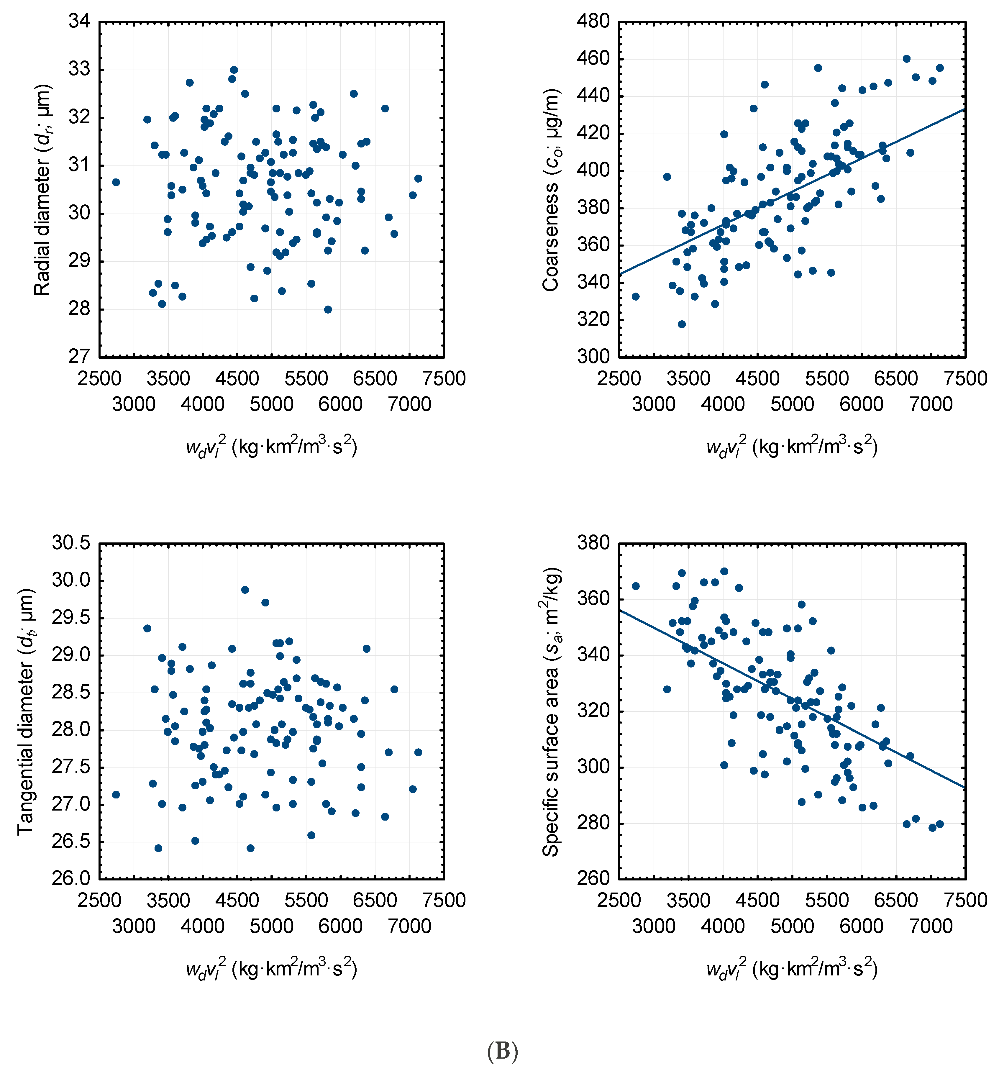
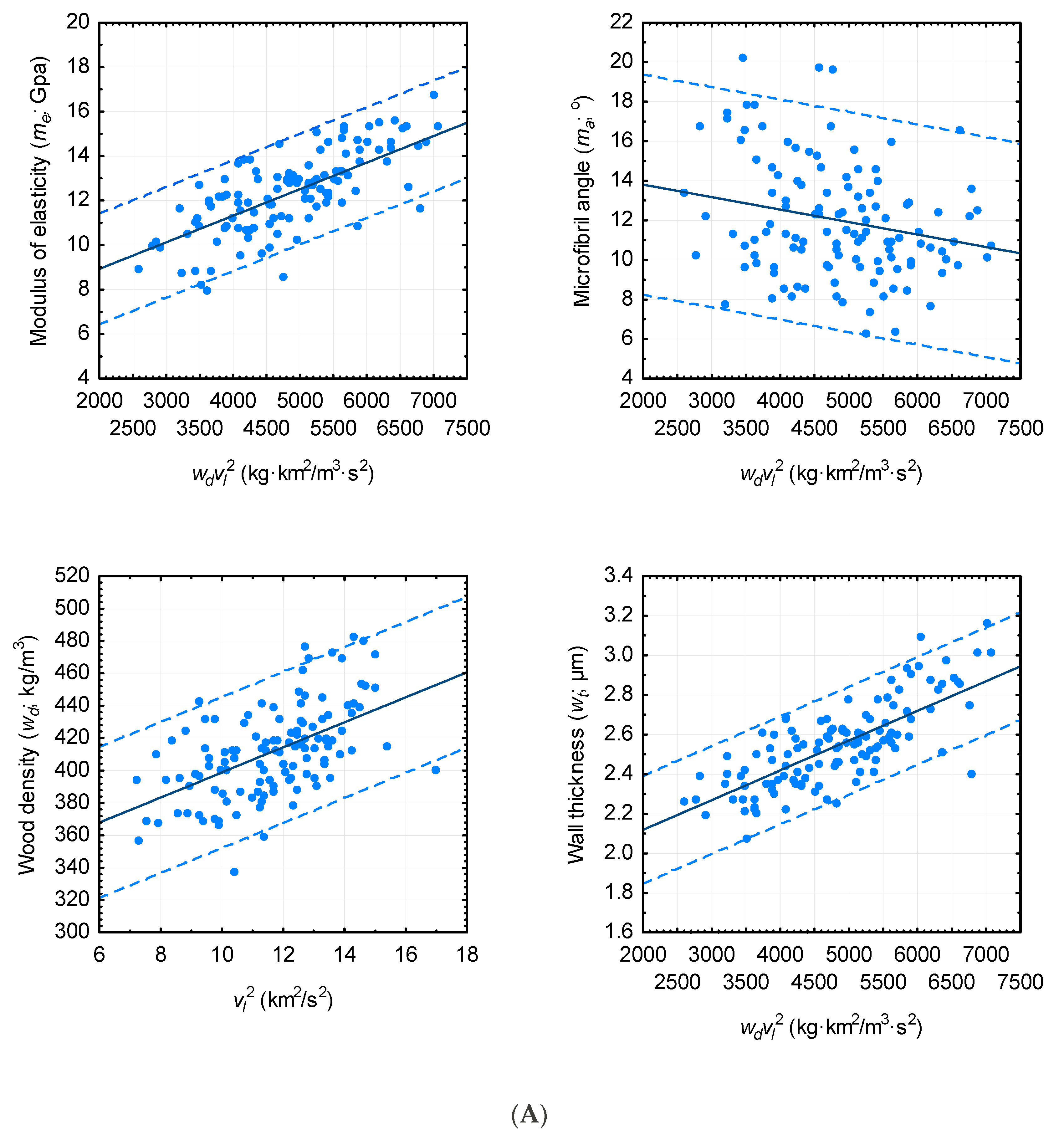
The attribute—acoustic velocity observational pairs within the calibration data subset for each of the 8 relationships evaluated are presented in Figure 1A,B. The successfully parameterized models are also superimposed on the observational pairs where applicable. Examination of the subgraphs for the attributes that were not successfully parameterized by the mixed-effects model specification (i.e., dr and dt; Table 7), reinforced the lack of a functional relationship between each of these attributes and density-weighted acoustic velocity: i.e., random cloud of the dr w d v l 2 and dt w d v l 2 observational pairs that were devoid of any obvious linear or nonlinear relationship. Conversely, for the attributes that were successfully parameterized by the mixed-effects model specification (i.e., me, ma, wd, wt, co, and sa; Table 7) which are superimposed on their respective subgraphs confirmed the statistical findings (i.e., relationships were unbiased and in accord with the me w d v l 2 , wd v l 2 , ma w d v l 2 , wt w d v l 2 , co w d v l 2 and sa w d v l 2 linear trends).

3.2. Goodness-of-fit and Lack-of-fit Assessment

The goodness-of-fit evaluation consisted of assessing the magnitude of the variability explained by the parameterized models when applied to the validation data subset. Specifically, the I2 statistic was calculated for the acoustic-based me, wd, ma, wt, co and sa mixed-effects models (Table 8). Results indicated that the models explained a relatively low to moderate level variation (ordered by magnitude): 8% for ma, 30% for wd, 43% for co, 44% for sa, 53% for me and 58% for wt. In agreement with expectation, the values for 5 of 6 attributes were slightly less than those observed for the relationships parameterized using the calibration data subset (cf. Table 7 versus Table 8). The exception being that of the result for me which was slightly greater than that derived from the calibration data subset. Based on the regression results for the linear relationship between the observed and predicted values, there was insufficient evidence to indicate systematic lack-of-fit for any of the 6 parameterized relationships: i.e., intercept and slope values were not significant (p > 0.01) different from zero and unity, respectively (sensu [31]). Similarly, based on the mean absolute biases and their associated 95% confidence intervals, there was no evidence of lack-of-fit for any of the 6 relationships (Table 8): mean absolute biases were not significantly (p ≤ 0.05) different from zero as inferred from the 95% confidence intervals. Although approximately equivalent results were obtained when assessing lack-of-fit using mean relative biases, the mean relative bias generated for the ma relationship was significantly (p ≤ 0.05) different from zero (Table 8).
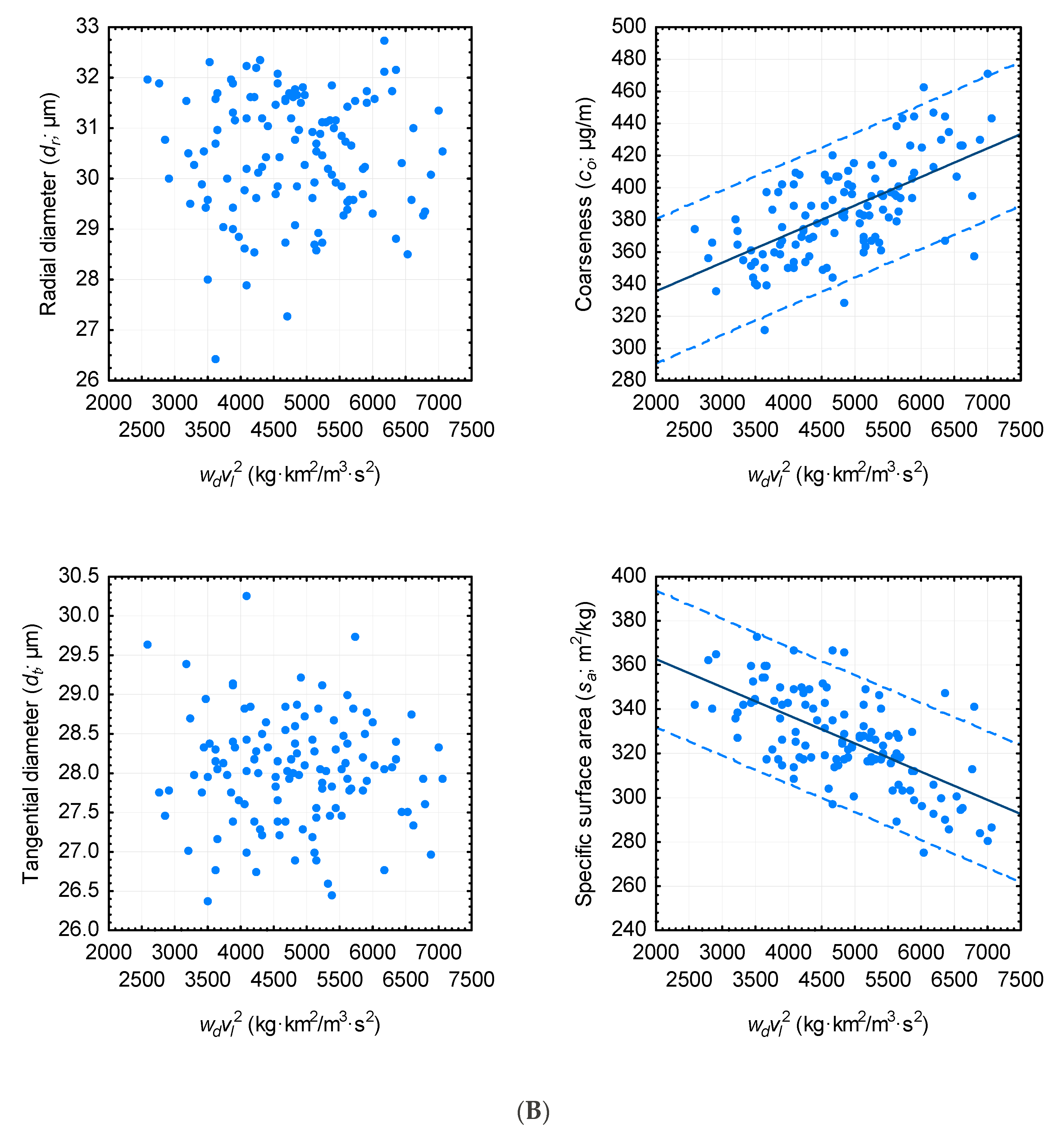
The density-weighed and density-unweighted acoustic velocity—attribute observational pairs within the validation data subset for each of the relationships including those that did not exhibit a significant relationship with acoustic velocity, are graphically presented in Figure 2A,B. The parameterized mixed-effects regression relationships derived using the calibration data subset were also superimposed on the me, wd, ma, wt, co and sa subgraphs. It was visually evident that the parameterized relationships were representative of the linear trends between the me w d v l 2 , wd v l 2 , ma w d v l 2 , wt w d v l 2 , co w d v l 2 and sa w d v l 2 observational pairs. The general concordance between the linear trends exhibited by the observational pairs and that established by the regressions, were also suggestive of the absence of systematic bias. For the attributes that were not successfully described by the mixed-effects model specification (i.e., dr and dt; Table 7), an examination of the subgraphs reconfirmed the statistical result, that is, there was a random scatter of dr w d v l 2 and dt w d v l 2 observational pairs devoid of discernable linear or nonlinear trends.

3.3. Predictive Ability

The predictive ability of the successfully parameterized mixed-effects models was quantified via the use of prediction and tolerance error intervals (Equations (9) and (10), respectively): mean bias ± 95% confidence limit. The intervals were generated from the absolute and relative bias values generated from the validation data subset. Statistically, these error intervals attempt to quantify the performance of the models when they are actually deployed [32]. Specifically, the prediction intervals quantify the boundaries of the expected range of absolute and relative errors when applying the models for a newly sampled jack pine log (e.g., there is 95% probability that the future error will be within the stated prediction interval). The tolerance intervals quantify the boundaries of the range of the expected population of absolute and relative errors which would be generated from the models when repeatedly deploying them to newly sampled jack pine log populations (e.g., there is 95% probability that 95% of all future errors will fall within the stated tolerance interval).
Accordingly, there is a 95% probability that a future error associated with a me, wd, ma, wt, co or sa prediction for a newly sampled jack pine log would be expected to fall within the following absolute and relative intervals (Table 8): (1) −2.5 ≤ me error (GPa) ≤ 2.5; −46.7 ≤ wd error (kg/m3) ≤ 46.4; −5.5 ≤ ma error (°) ≤ 5.6; −0.3 ≤ wt error (µm) ≤ 0.3; −45.3 ≤ co error (µg/m) ≤ 44.5; and −30.7 ≤ sa error (m2/kg) ≤ 31.2; and (2) −21.6 ≤ me error (%) ≤ 23.5; −11.0 ≤ wd error (%) ≤ 11.6; −44.1 ≤ ma error (%) ≤ 56.1; −10.5 ≤ wt error (%) ≤ 10.8; −11.5 ≤ co error (%) ≤ 12.0; and −9.2 ≤ sa error (%) ≤ 9.8. Similarly, based on the tolerance error intervals as presented in Table 8, there is a 95% probability that 95% of all future errors generated from the me, wd, ma, wt, co and sa models would fall within the following absolute and relative intervals: (1) −2.8 ≤ me error (GPa) ≤ 2.7; −51.7 ≤ wd error (kg/m3) ≤ 51.5; −6.1 ≤ ma error (°) ≤ 6.2; −0.3 ≤ wt error (µm) ≤ 0.3; −50.2 ≤ co error (µg/m) ≤ 49.4; and −34.1 ≤ sa error (m2/kg) ≤ 34.5; and (2) −24.0 ≤ me error (%) ≤ 26.0; −12.2 ≤ wd error (%) ≤ 12.8; −49.5 ≤ ma error (%) ≤ 61.5; 11.7 ≤ wt error (%) ≤ 12.0; −12.8 ≤ co error (%) ≤ 13.3; and −10.2 ≤ sa error (%) ≤ 10.8. Although these intervals also reveal that the parameterized equations would generate unbiased predictions, the level of predictive accuracy attained would vary widely among the attributes (e.g., sa > wt > wd > co >> me >>> ma based on the width of relative error tolerance intervals).

3.4. Predictive Performance of Parameterized Models When Deploying Acoustic Generated Wood Density Estimates

Employing the validation data subset, the empirical performance of the density-weighted models in cases where an acoustic-based wood density estimate was used as a surrogate for a Silviscan-based density estimate, was also evaluated. Specifically, based on the functional expressions, me, ma, wt, co, sa = f ( γ ^ 0 , 1 , w ^ d v l 2 ) where w ^ d is derived from the wd = f ( γ ^ 0 , 1 , v l 2 ) relationship, the following set of computations were carried out: (1) inputting the acoustic velocity measurement value for each log in the validation data subset into the parameterized wd model (Table 7) and generating associated estimates for each attribute; and (2) given (1), treating these resultant attribute estimates as predicted values and the corresponding Silviscan-determined estimates as observed values, absolute and relative biases and associated 95% confidence, and 95% prediction and tolerance intervals, were calculated via the deployment of the computational structure given by Equations (7)–(11).
Upon review of the resulting predictive performance metrics as provided in Table 9, lack-of-fit issues were non-concerning for either of the error measures: 95% confidence intervals indicated that the mean absolute and relative biases were not significantly (p ≤ 0.05) different from zero. Numerically, the magnitude of error generated when estimating me, ma, wt, co and sa for a newly sampled jack pine log deploying the acoustic-based density estimate, would be captured within the following absolute and relative prediction error intervals: (1) −2.8 ≤ me error (GPa) ≤ 2.7; −5.5 ≤ ma error (°) ≤ 5.6; −0.3 ≤ wt error (µm) ≤ 0.3; −51.8 ≤ co error (µg/m) ≤ 50.9; and −36.5 ≤ sa error (m2/kg) ≤ 37.0; and (2) −23.5 ≤ me error (%) ≤ 25.8; −43.7 ≤ ma error (%) ≤ 55.7; −10.5 ≤ wt error (%) ≤ 10.8; −13.1 ≤ co error (%) ≤ 13.7; and −10.9 ≤ sa error (%) ≤ 11.7. Similarly, the corresponding 95% tolerance intervals for which 95% of all future errors would be expected to be captured are delineated as follows: (1) −3.1 ≤ me error (GPa) ≤ 3.0; −6.1 ≤ ma error (°) ≤ 6.2; −0.3 ≤ wt error (µm) ≤ 0.3; −57.4 ≤ co error (µg/m) ≤ 56.5; and −40.5 ≤ sa error (m2/kg) ≤ 41.0; and (2) −26.2 ≤ me error (%) ≤ 28.4; −49.1 ≤ ma error (%) ≤ 61.1; −11.7 ≤ wt error (%) ≤ 12.0; −14.6 ≤ co error (%) ≤ 15.2; and −12.2 ≤ sa error (%) ≤ 12.9. In summary, these results suggest that the attribute prediction models in which an acoustic-based wood density estimate is deployed, would yield unbiased predictions which would be slightly less precise than that attained when using a Silviscan-derived or equivalent density estimate, and would exhibit a similar among-attribute performance ranking (cf. Table 8 versus Table 9).

4. Discussion

4.1. Hierarchical Mixed-Effects Acoustic-Based Attribute Prediction Models for Jack Pine

The mixed-effects linear model for the primary relationship between the dynamic modulus of elasticity and density-weighted acoustic velocity (me = f ( γ ^ 0 , 1 , w d v l 2 ) ) explained 47% of the variation in the me for the logs within the calibration data subset (Table 7) and 53% of the variation in the me for the logs within the validation data subset (Table 8). Based on the logs within the validation data subset, the model generated unbiased predictions when assessed using both absolute and relative error measures. The tolerance intervals indicated that 95% of the absolute and relative errors generated from repeatedly applying the parameterized model to a new sample population of jack pine logs would be expected (95% probability level) not to exceed ±2.8 GPa and ±25.0% respectively, when using Silviscan-equivalent wd estimate (Table 8). For the deployment scenario in which an acoustic-based wood density estimate is employed as a surrogate measure for its Silviscan-based counterpart, the model’s predictions would be similarly unbiased (Table 9). However, the predictions would be less precise as evident from the wider tolerance intervals for absolute and relative error that were generated when using the acoustic-based density estimate (i.e., 95% tolerance limits for error of ±3.1 GPa and ±27.3%, respectively; Table 9). Newton [15] reported slightly better results in a similarly structured analysis of red pine logs in terms of explanatory power (e.g., explaining 71% of variation in me for red pine logs versus 50% of variation in me for jack pine logs) and precision of predictions when deploying either a Silviscan-equivalent estimate of wood density (e.g., relative tolerance error intervals of ±19% for red pine versus ± 25% for jack pine) or acoustic-based estimate (e.g., relative tolerance error intervals of ±19% for red pine versus ± 27% for jack pine).
The results for the mixed-effects linear regression model for the relationship between wood density and acoustic velocity (wd = f ( γ ^ 0 , 1 , v l 2 ) ), revealed that the parameterized model generated unbiased predictions (Table 7 and Table 8). Overall, however, the model performed moderately in terms of (1) explanatory power given that only 32% and 31% of the wd variation for the logs within the calibration and validation data subsets, respectively, was explained (Table 7 and Table 8), and (2) predictive performance given that 95% of absolute and relative errors generated from repeatedly applying the equation to a new sample population of logs would be expected (95% probability level) not to exceed ±51.6 kg/m3 or ±12.5%, respectively (Table 8). Considerably better results were reported previously for red pine logs [15] in terms of explanatory power (e.g., explaining 80% of variation in wd for red pine logs versus 31% of variation in wd for jack pine logs). However, differences in the precision of the predictions were only marginally better (e.g., relative tolerance error intervals of ±10% for red pine versus ± 13% for jack pine).
Although the results for the relationship where microfibril angle is expressed as a function of density-weighted acoustic velocity (ma = f ( γ ^ 0 , 1 , w d v l 2 ) ) generated unbiased predictions (Table 7 and Table 8), the parameterized model exhibited a low level of explanatory power and a relatively high degree of imprecision. Specifically, the model only explained 8% of the variation in ma for the logs within both the calibration and validation data subsets, respectively (Table 7 and Table 8). The predictive intervals indicated that 95% of absolute and relative errors generated from repeatedly applying the equation to a new sample population of logs would be expected (95% probability level) not to exceed (1) ±6.2 ° and ±55.5%, respectively, when using Silviscan-equivalent wd estimates (Table 8), and (2) ±6.2 ° and ±55.1%, respectively, when deploying acoustic-based wood density estimates. Although these weak results are superior to those obtained previously for red pine logs in which no viable acoustic-based relationship was found for microfibril angle [15], the results are inferior to the level of variation described by the acoustic-based relationship reported in other studies (e.g., 86% for radiata pine logs [6]).
The relationship for cell wall thickness (wt = f ( γ ^ 0 , 1 , w d v l 2 ) ) exhibited the highest levels of explanatory power as evident from the level of variation explained: 60% and 58% for the calibration and validation data subsets, respectively (Table 7 and Table 8). Furthermore, the parameterized model exhibited no lack-of-fit issues and produced unbiased predictions at a relatively high level of precision. Specifically, 95% of absolute and relative errors generated from repeatedly applying the equation to a new sample population of jack pine logs would be expected (95% probability level) to not exceed ±0.3 µm and ±11.8%, respectively, when using Silviscan-equivalent or acoustic generated wd estimates (Table 8 and Table 9). Newton [15] reported a superior result for red pine logs in terms of explanatory power (e.g., explaining 90% of variation in wt for red pine logs versus 59% of variation in wt for jack pine logs), but much less so in terms of predictive precision. For example, relative tolerance error intervals of ±9% for red pine versus ±12% for jack pine when deploying a Silviscan-equivalent estimate of wood density, and ±12% for red pine versus ±12% for jack pine when using an acoustic-based estimate. The graphical and statistical results for the relationships in which radial and tangential diameters were expressed as functions of density-weighted acoustic velocity, did not support the existence of viable relationships for these attributes. This result is similar to that obtained for red pine logs (i.e., [15]). Combining these regression results with the observed lack of linear associations exhibited in the scatterplots (Figure 1 and Figure 2 for jack pine logs; and Figure 1 and Figure 2 for red pine logs in [15]), suggest that these attributes may be intrinsically unrelated to acoustic velocity for these species.
The regression relationships for fiber coarseness and specific surface area (co, sa = f ( γ ^ 0 , 1 , w d v l 2 ) ) exhibited moderate levels of explanatory power (Table 7 and Table 8): (1) 46% and 43% of the variation in fiber coarseness was explained for the logs within the calibration and validation data subsets, respectively; and (2) 50% and 44% of the variation in specific surface area was explained for the logs within the calibration and validation data subsets, respectively. These parameterized models produced unbiased and relative precise predictions when compared with the other attribute models. For the fiber coarseness model, 95% of absolute and relative errors generated from repeatedly applying the parameterized equation to a new sample population of logs would be expected (95% probability level) not to exceed (1) ±49.8 µg/m and ±13.0%, respectively, when using Silviscan-equivalent wood density estimates (Table 8), and (2) ±57.0 µg/m and ±14.9%, respectively, when deploying acoustic-based wood density estimates (Table 9). Similarly, for the model developed for specific surface area, the corresponding precision limits for absolute and relative error were (1) ±34.3 m2/kg and ±10.5%, respectively, when using Silviscan-equivalent wood density estimates (Table 8), and (2) ±40.7 m2/kg and ±12.5%, respectively, when deploying acoustic-derived wood density estimates (Table 9).
In relation to acoustic-based prediction of fiber coarseness, Newton [15] reported much improved results for red pine logs in terms of explanatory power (e.g., explaining 81% of variation in co for red pine logs versus 44% of variation in co for jack pine logs) but again much less so in terms of predictive precision (e.g., relative tolerance error intervals of ±12% for red pine versus ±13% for jack pine when deploying a Silviscan-equivalent estimate of wood density, and ±14% for red pine versus ±15% for jack pine when using an acoustic-based estimate). In comparison of the model developed for predicting specific surface area for red pine logs, the result was considerably superior in terms of explanatory power (e.g., 84% of the variation in sa explained for red pine logs versus 47% of the variation in sa explained for jack pine logs). However, similar to the interspecies comparison of the coarseness model, the difference in predictive ability was minimal between the species: (1) relative tolerance error intervals of ±8% for red pine versus ±11% for jack pine when deploying a Silviscan-equivalent estimate of wood density, and (2) ±10% for red pine versus ±13% for jack pine when using an acoustic-based estimate.

4.2. Potential Utility of the Expanded Acoustic-Based Inferential Framework for Jack Pine

Estimation of the modulus of elasticity is of primary importance in log-segregation operations where the objective is to forecast the potential type and grade of extracted solid wood products (e.g., dimension lumber). However, other wood attributes (e.g., wood density, microfibril angle, tracheid dimensions) and derived composite metrics (e.g., fiber coarseness and specific surface area), are also prime determinates of end-product potential (sensu Table 1). Consequently, the expanded acoustic inferential framework presented in this study along with its empirical validation for six of the eight jack pine attributes examined (dynamic modulus of elasticity, wood density, microfibril angle, cell wall thickness, fiber coarseness and specific surface area), yields a more comprehensive system for non-destructive forecasting of end-product potential than systems based solely on wood stiffness (modulus of elasticity). Operationally, however, the in-forest deployment of the parameterized relationships will be largely dependent on the objectives and precision requirements of the end-user. For example, the relative error intervals were quite large for me and ma as exemplified by the resultant tolerance errors of ±25% and ±56%, respectively, when using a Silviscan-equivalent wood density estimate (Table 8), and ±27% and ±55%, respectively, when using an acoustic-based wood density estimate (Table 9). Thus, the ability to stratify individual jack pine logs into narrow-grade class-based acoustic estimates of me and ma would be difficult if not impossible. However, in situations for which the objective is to segregate groups of logs into end-product categories according to their average attribute values, then the magnitude of estimation error associated with the acoustic-based population mean estimates may be more operationally acceptable. For example, the mean absolute and relative error to be expected when collectively sampling 30 new jack pine logs deploying an acoustic-based wood density estimate would be, respectively, 0.6 GPa and 5% for me, and 1° and 10% for ma (Table 9).
Comparably, the relative tolerance error intervals for wd, wt, co and sa were considerably less (i.e., errors in the order of ±10 to ±15% (Table 8)). Thus, depending on the specified width of the wd, wt, co and sa intervals the end-user employs to designate logs into specific end-product categories or a binary grade class, differentiating logs according to these attribute predictions may be feasible. Similarly, at the stand-level where the objective is to classify a population of logs in a specific end-product category based on their mean wd, wt, co or sa values, the precision of the estimates would be improved considerably. For example, the mean absolute and relative error to be expected when collectively sampling 30 new jack pine logs deploying an acoustic-based wood density estimate would be respectively, 0.1 µm and 2% for wt, 10.4 µg/m and 3% for co, and 7.5 m2/kg and 2% for sa (Table 9).
More generally however, based on the explanatory power and precision of acoustic-based attribute prediction models developed to date, increasing the precision of the point-estimates derived from acoustic-based models will be required if they are to be used to stratify individual logs into grade categories given the relatively narrow range of static modulus of elasticity values that currently delineate product grade classes. For example, the mean difference between the 14 machine stress-rated (MSR) lumber grade categories established for Canadian softwood species [34] is approximately 0.7 GPa and hence the explicit stratification of individual logs into such narrow-width grade classes would not be possible given the empirical results to date. Even if it is assumed that the dynamic estimate is equivalent to its static counterpart which in turn is reflective of the actual end-product-based value, the precision of most acoustic-based estimates would be inadequate for stratifying logs into MSR-based classes (e.g., ±3 GPa expected error for individual jack pine logs; Table 9). Thus reducing the number of grade categories from 14 to a smaller number of discrete quality classes based on the expected prediction error range(s) through clustering, and (or) using multiple individual log estimates to generate a mean site, landing or log pile value, may represent a viable alternative when using the acoustic approach in log-segregation operations for jack pine.
Further research into analytical advancements that increase the amount of variability explained and decrease the standard error of estimate, possibly by including covariates within the acoustic-attribute model specification as suggested by Bérubé-Deschênes et al. [35] and Butler et al. [36], may be warranted. Acoustic velocity is known to be affected by a multitude of internal and external factors which includes knot distributions, embedded voids, environmental conditions during acoustic sampling (temperature and moisture conditions), tree size, local competition, and overall site conditions (e.g., [35,37,38]). Provision of operational solutions for minimizing these effects could improve the predictive accuracy of acoustic-based attribute estimation. Recent results examining the effect of xylem temperature and moisture on acoustic velocity within standing semi-mature jack pine trees during the vegetative growing season indicated that acoustic velocity declined in linear fashion with increasing temperature; however, moisture had no appreciable influence [39]. However, the temperature effect was not of consequential significance except when temperatures approached their seasonal extremities. Assuming similar inferences apply to jack pine logs, suggest that acoustic log samplers could treat such variation as a source of random error of minimal importance providing xylem temperatures did not approach their seasonal minimums (<5 °C) or maximums (>30 °C). In cases were temperature effects were of concern, the standardization equation for adjusting acoustic velocities to a reference xylem temperature of 20 °C could be deployed [39].

4.3. Similarities and Differences between Tree and Log Acoustic-Based Attribute Relationships

The time-of-flight acoustic approach to estimating the internal attributes within standing trees employs the dilatational stress wave velocity (vd) which transverses the breast-height (1.3 m) region of the main stem [40]. This acoustic velocity measurement when weighted by wood density is also related to the modulus of elasticity as described by a functional specification, similar to that given by Equation (1) (i.e., replacing vl by vd). This primary relationship for standing trees can be also potentially expanded to include a similarly structured suite of secondary relationships as that presented in this study for logs (e.g., [16]).
Conceptually, the resonance-based acoustic velocity approach is considered to yield a more representative estimate of the fiber attributes within the xylem tissue than those estimates derived from the time-of-flight approach. This is principally because the mean velocity estimate is derived from many acoustic pulses resonating longitudinally throughout the log rather than the velocity of a single wave front moving between two points within the main stem of a standing tree [41]. The empirical validity of this inference can be partially tested by assessing the differences between the tree and log acoustic-based attribute prediction models parameterized using the same sample tree population. Contrasting the results derived from a companion analysis which assessed the time-of-flight acoustic relationships deploying the same suite of attributes and sample tree population which were measured at the same time [42], revealed that the time-of-flight-based relationships were mostly superior in terms of explanatory power. Specifically, the percentage of attribute variation explained by the dilatational (tree) and longitudinal (log) acoustic relationships were respectively: 71% versus 50% for me; 30% versus 31% for wd; 19% versus 8% for ma; 66% versus 59% for wt; 42% versus 44% for co; and 61% versus 47% for sa. However, conversely, in terms of predictive precision, the comparison between the log and tree models revealed minimal differences. The error arising from using a newly sampled acoustic velocity measurement used to estimate me, wd, ma, wt, co and sa for standing trees and derived logs would be expected at the 95% confidence level to fall within the respective relative error limits of ±25% versus ±21% for me, ±13% versus ±14% for wd, ±56% versus ±47% for ma, ±12% versus ±11% for wt, ±13% versus ±12% for co, and ±10% versus ±10% for sa. These similarities in terms of the predictive performance between the tree and log-based acoustic approaches for estimating attributes within the same species (jack pine) while attaining contrasting results between species (jack pine versus red pine for a given time-of-flight- or resonance-based relationship), suggest that acoustic-based attribute relationships may be intrinsic to a given species irrespective of either of these wave types.

4.4. Advancing Acoustic-Based Attribute Estimation

The resonance-based acoustic approach to estimating internal fiber attributes within logs and associated demonstrations of its utility in segregation, allocation and merchandizing operations have been presented to the forest management community through various case studies (e.g., [41,43,44] and comprehensive literature reviews (e.g., [11,17]). These contributions have mostly focused on the merits of estimating the modulus of elasticity and using it, or its surrogates, to forecast end-product potential. These include (1) treating wood density as a constant and inferring wood stiffness indirectly from acoustic velocity (e.g., implicitly based on the underlying theoretical relationship expressed by Equation (1)), (2) estimating wood stiffness using parameterized regression models in which the dynamic modulus of elasticity is expressed as a function of acoustic velocity and wood density (e.g., explicitly based on the conceptual formulation (Equation (1)), and (3) directly forecasting wood stiffness using relationships that explicitly relate the static modulus of elasticity of a given end-product (e.g., measured using static bending tests of sawn boards) to acoustic velocity. This last approach while the most informative is also the least developed. Consequentially, the full potential of in-forest acoustic-based forecasting of end-product potential has not been fully realized. Determination and quantification of the explicit relationship between log-based acoustic velocity measures and actual performance-based metrics within the derived manufactured end-product are also required. Preliminary results from several studies in which the static modulus of elasticity within dimensional lumber products have been explicitly related to log-based acoustic velocity measures have been positive. These include statistically viable relationships reported for balsam fir (Abies balsamea (L.) Mill.) and white spruce (Picea glauca (Moench) Voss.) [45], radiata pine [46], Douglas fir ((Pseudotsuga menziesii (Mirb.) Franco) [47], and loblolly pine (Pinus taeda L.) [48].
Similarly, previous research has shown that several important performance metrics associated with pulp and paper end-products are also empirically related to acoustic velocity measurements taken on logs. Clark et al. [48] found that fiber length, pulp strength and various handsheet properties derived from radiate pine logs varied systematically with acoustic velocity. Bradley et al. [49] demonstrated that the variation in the pulp quality (freeness) for radiata pine logs could be considerably reduced by stratifying the logs according to their acoustic velocity values before processing. Although beyond the scope of this study, establishment of a broader range of more explicit relationships between log-based acoustic velocity measures and attribute-derived performance metrics within actual manufactured end-products, would be an area worthy of further investigation. As these past studies have shown, in-forest acoustic velocity stratification of log populations not only improves segregation efficiency at the time of harvest but also assists in reducing the variation in end-product quality during the manufacturing and merchandizing stages.
In-forest acoustic log grading has been increasingly used to compliment visual-based approaches in the pursuit of deriving economically efficient sorting networks. This remains an iterative and ongoing process in wood allocation decision-making where the objective is to increase operational efficiency within the upstream portion of the forest products supply chain (sensu [50]). Mechanized acoustic sampling has also advanced to the point where onboard resonance tools have been installed directly on harvesting machines where logs are immediately sorted upon bucking according to their end-product potential (e.g., [51]). Although these innovations have advanced the in-forest non-destructive approach to log grading and sorting, the acoustic approach has been largely limited to providing a single measure of internal wood quality, that being wood stiffness. Thus, the confirmatory empirical results presented in this study for jack pine and previous for red pine logs [15] are collectively supportive of an expanded acoustic-based inferential framework in which estimates for a multitude of end-product-based attribute determinates can be attained: e.g., wood density, microfibril angle, tracheid wall thickness, fiber coarseness, and specific surface area, in addition to the dynamic modulus of elasticity (wood stiffness). Although further research is required to fully realize the benefits of this empirical-based framework, the ability to non-destructively forecast a wide array of commercially relevant attributes could have consequential potential utility in advancing the acoustic approach in forest operations.

5. Conclusions

Given the wide spread occurrence of jack pine across the boreal landscape combined with the vast array of potential end-products it can produce, inclusive of solid wood products (e.g., dimensional lumber) and associated mill-work derivatives (window frames, doors, shelving, moldings, and paneling, and composite lumber products such as glulam-based beams, headers and heavy trusses and finger-jointed joists and rafters), and pulp-derived products such as paperboards, newsprint, facial tissues and specialized coated papers [52], the species has become the dominant feedstock species for numerous industrial conversion facilities. However, this diversity of end-products complicates in-forest segregation, allocation, and merchandizing decision-making. Hence the provision of enhanced operational intelligence arising from in-forest forecasts of end-product potential of harvested logs through non-destructive acoustic-based methods, may yield increased efficiencies within the upper portion of the jack pine forest products supply chain. Consequentially, the development and evaluation of a suite of acoustic-based models for predicting the principal attributes governing end-product potential for jack pine as presented in this study, represents an incremental contribution towards more informed decision-making. Specifically, deploying a mixed-effects linear modeling approach combined with cross-validation techniques, viable forecasting models for predicting the dynamic modulus of elasticity, wood density, microfibril angle, cell wall thickness, fiber coarseness and specific surface area were developed. Although these positive results confer additional empirical support for the proposed acoustic-based inferential framework, further research in the areas of accounting for environmentally induced wave variation, specifying end-product-based design thresholds, and explicitly establishing linkages between log-based attribute estimates and those within recoverable end-products, would be beneficial. Collectively, the results presented here for jack pine not only provides the prerequisite parameterized relationships for improving in-forest segregation and allocation decision-making but also contributes to solidifying the empirical foundation of the expanded acoustic-based inferential framework.

Funding

Canadian Wood Fiber Centre, Canadian Forest Service, Natural Resources Canada.

Acknowledgments

The author expresses his appreciation to: (1) Mike Laporte (retired) of the Canadian Wood Fiber Centre, Canadian Forest Service (CFS), Natural Resources Canada (NRCan), and Gordon Brand of the Great Lakes Forestry Centre, CFS, NRCan for field and laboratory data acquisition support; (2) Dr. Tong and Ny Nelson at FPInnovations Inc., Vancouver, British Columbia, Canada, for completing the SilviScan-3 analysis, (3) Canadian Wood Fiber Centre, CFS, NRCan for fiscal support; and (4) anonymous journal reviewers for constructive and insightful comments and suggestions.

Conflicts of Interest

The author declares no conflict of interest.

References

  1. Emmett, B. Increasing the value of our forest. For. Chron. 2006, 82, 3–4. [Google Scholar] [CrossRef]
  2. Emmett, B. Perspectives on sustainable development and sustainability in the Canadian forest sector. For. Chron. 2006, 82, 40–43. [Google Scholar] [CrossRef] [Green Version]
  3. Zhang, S.Y.; Chauret, G.; Ren, H.Q.; Desjardins, R. Impact of plantation black spruce initial spacing on lumber grade yield, bending properties and MSR yield. Wood Fibre Sci. 2002, 34, 460–475. [Google Scholar]
  4. Tsehaye, A.; Buchanan, A.H.; Walker, J.C.F. Sorting of logs using acoustics. Wood Sci. Technol. 2000, 34, 337–344. [Google Scholar] [CrossRef]
  5. Carter, P.; Briggs, D.; Ross, R.J.; Wang, X. Acoustic testing to enhance western forest values and meet customer wood quality needs. In Productivity of Western Forests: A Forest Products Focus; Harrington, C.A., Schoenholtz, S.H., Eds.; Gen. Tech. Rep. PNW-GTR-642; USDA, Forest Service, Pacific Northwest Research Station: Portland, OR, USA, 2005; pp. 121–129. [Google Scholar]
  6. Wang, X.; Carter, P.; Ross, R.J.; Brashaw, B.K. Acoustic assessment of wood quality of raw materials: A path to increased profitability. For. Prod. J. 2007, 57, 6–14. [Google Scholar]
  7. National Lumber Grades Authority (NLGA). Standard Grading Rules for Canadian Lumber; NLGA: Surrey, BC, Canada, 2014. [Google Scholar]
  8. Defo, M. SilviScan-3—A Revolutionary Technology for High-Speed Wood Microstructure and Properties Analysis. Midis de al Foresterie. UQAT. Available online: http://chaireafd.uqat.ca/midiForesterie/pdf/ 20080422PresentationMauriceDefo.pdf (accessed on 1 October 2018).
  9. Wang, X.; Ross, R.J.; Mattson, J.A.; Erickson, J.R. Nondestructive evaluation techniques for assessing modulus of elasticity and stiffness of small-diameter logs. For. Prod. J. 2002, 52, 79–85. [Google Scholar]
  10. Dickson, R.L.; Raymond, C.A.; Joe, B.; Wilkinson, C.A. Segregation of Eucalyptus dunnii logs using acoustics. For. Ecol. Manag. 2003, 179, 243–251. [Google Scholar] [CrossRef]
  11. Ross, R.J. Nondestructive Evaluation of Wood, 2nd ed.; General Technical Report FPL-GTR-238; USDA, Forest Service, Forest Products Laboratory: Madison, WI, USA, 2015; p. 169.
  12. Legg, M.; Bradley, S. Measurement of stiffness of standing trees and felled logs using acoustics: A review. J. Acoust. Soc. Am. 2016, 139, 588–604. [Google Scholar] [CrossRef] [PubMed] [Green Version]
  13. Raymond, C.A.; Joe, B.; Evans, R.; Dickson, R.L. Relationship between timber grade, static and dynamic modulus of elasticity, and Silviscan properties for Pinus radiata in New SouthWales. N. Z. J. For. Sci. 2007, 37, 186–196. [Google Scholar]
  14. Newton, P.F. Development trends of black spruce fibre attributes in maturing plantations. Int. J. For. Res. 2016, 1–12. [Google Scholar] [CrossRef]
  15. Newton, P.F. Predictive relationships between acoustic velocity and wood quality attributes for red pine logs. For. Sci. 2017, 63, 504–517. [Google Scholar] [CrossRef]
  16. Newton, P.F. Acoustic-based non-destructive estimation of wood quality attributes within standing red pine trees. Forests 2017, 8, 380. [Google Scholar] [CrossRef]
  17. Wang, X. Acoustic measurements on trees and logs: A review and analysis. Wood Sci. Technol. 2013, 475, 965–975. [Google Scholar] [CrossRef]
  18. Brashaw, B.K.; Bucur, V.; Divos, F.; Goncalves, R.; Lu, J.; Meder, R.; Yin, Y. Nondestructive testing and evaluation of wood: A worldwide research update. For. Prod. J. 2009, 59, 7–14. [Google Scholar]
  19. Wang, X.; Senalik, C.A.; Ross, R.J. (Eds.) 20th International Nondestructive Testing and Evaluation of Wood Symposium; General Technical Report FPL-GTR-249; USDA, Forest Service, Forest Products Laboratory: Madison, WI, USA, 2017; p. 539.
  20. McKinnon, L.M.; Kayahara, G.J.; White, R.G. Biological Framework for Commercial Thinning Evenaged Single-Species Stands of Jack Pine, White Spruce, and Black Spruce in Ontario; Report TR-046; Ontario Ministry of Natural Resources, Northeast Science and Information Section: Timmins, ON, Canada, 2006; p. 130.
  21. Carmean, W.H.; Niznowski, G.P.; Hazenberg, G. Polymorphic site index curves for jack pine in Northern Ontario. For. Chron. 2001, 77, 141–150. [Google Scholar] [CrossRef] [Green Version]
  22. Rowe, J.S. Forest Regions of Canada; Publication No. 1300; Government of Canada, Department of Environment, Canadian Forestry Service: Ottawa, ON, Canada, 1972.
  23. Evans, R. Rapid measurement of the transverse dimensions of tracheids in radial wood sections from Pinus radiata. Holzforschung 1994, 48, 168–172. [Google Scholar] [CrossRef]
  24. Siau, J.F. Wood: Influence of Moisture on Physical Properties; Virginia Polytechnic Institute and State University, Department of Wood Science and Forest Products: Blacksburg, VA, USA, 1995.
  25. Evans, R.; Hughes, M.; Menz, D. Microfibril angle variation by scanning X-ray diffractometry. Appita 1999, 52, 363–367. [Google Scholar]
  26. Evans, R. Wood stiffness by X-ray diffractometry. In Characterization of the Cellulosic Cell Wall; Stokke, D.D., Groom, L.H., Eds.; Wiley: Hoboken, NJ, USA, 2006; pp. 138–146. [Google Scholar]
  27. Evans, R.; Downes, G.; Menz, D.; Stringer, S. Rapid measurement of variation in tracheid transverse dimensions in a radiata pine tree. Appita 1995, 48, 134–138. [Google Scholar]
  28. Raudenbush, S.W.; Bryk, A.S. Hierarchical Linear Models: Applications and Data Analysis Methods, 2nd ed.; Sage: Newbury Park, CA, USA, 2002; p. 485. [Google Scholar]
  29. Raudenbush, S.W.; Bryk, A.S.; Cheong, Y.F.; Congdon, R.T.; Toit, M., Jr. HLM 7—Hierarchical Linear and Nonlinear Modeling; Scientific Software International Inc.: Lincolnwood, IL, USA, 2011; p. 360. [Google Scholar]
  30. Gujarati, D.N. Essentials of Econometrics, 3rd ed.; McGraw-Hill/Irwin Inc.: New York, NY, USA, 2006; p. 553. [Google Scholar]
  31. Ek, A.R.; Monserud, R.A. Performance and comparison of stand growth models based on individual tree and diameter-class growth. Can. J. For. Res. 1979, 9, 231–244. [Google Scholar] [CrossRef]
  32. Reynolds, M.R., Jr. Estimating the error in model predictions. For. Sci. 1984, 30, 454–469. [Google Scholar]
  33. Gribko, L.S.; Wiant, H.V., Jr. A SAS template program for the accuracy test. Compiler 1992, 10, 48–51. [Google Scholar]
  34. National Lumber Grades Authority (NLGA). Special Products Standard for Machine Graded Lumber; NLGA: Surrey, BC, Canada, 2013. [Google Scholar]
  35. Bérubé-Deschênes, A.; Franceschini, T.; Schneider, R. Factors affecting plantation grown white spruce (Picea glauca) acoustic velocity. J. For. 2016, 114, 629–637. [Google Scholar] [CrossRef]
  36. Butler, M.A.; Dahlen, J.; Eberhardt, T.L.; Montes, C.; Antony, F.; Daniels, R.F. Acoustic evaluation of loblolly pine tree-and lumber-length logs allows for segregation of lumber modulus of elasticity, not for modulus of rupture. Ann. For. Sci. 2017, 74, 1–15. [Google Scholar] [CrossRef]
  37. Kang, H.; Booker, R.E. Variation of stress wave velocity with MC and temperature. Wood Sci. Technol. 2002, 36, 41–54. [Google Scholar] [CrossRef]
  38. Chauhan, S.S.; Walker, J.C.F. Variations in acoustic velocity and density with age, and their interrelationships in radiata pine. For. Ecol. Manag. 2006, 229, 388–394. [Google Scholar] [CrossRef]
  39. Newton, P.F. Quantifying the effects of wood moisture and temperature variation on time-of-flight acoustic velocity measures within standing red pine and jack pine trees. Forests 2018, 9, 527. [Google Scholar] [CrossRef]
  40. Wessels, C.B.; Malan, F.S.; Rypstra, T. A review of measurement methods used on standing trees for the prediction of some mechanical properties of timber. Eur. J. For. Res. 2011, 130, 881–893. [Google Scholar] [CrossRef]
  41. Wang, X.; Carter, P. Acoustic assessment of wood quality in trees and logs. In Nondestructive Evaluation of Wood; Ross, R.J., Ed.; General Technical Report FPL-GTR-238; USDA, Forest Service, Forest Products Laboratory: Madison, WI, USA, 2015; pp. 87–101. [Google Scholar]
  42. Newton, P.F. In-forest acoustic-based prediction of commercially-relevant wood quality attributes within standing jack pine trees. Forests 2018. in preparation. [Google Scholar]
  43. Walker, J.C.F.; Nakada, R. Understanding corewood in some softwoods: A selective review on stiffness and acoustics. Int. For. Rev. 1999, 1, 251–259. [Google Scholar]
  44. Harris, P.; Petherick, R.; Andrews, M. Acoustic resonance tools. In Proceedings of the 13th International Symposium on Nondestructive Testing of Wood; Forest Products Society: Berkeley, CA, USA, 2003; pp. 195–201. [Google Scholar]
  45. Ross, R.J.; McDonald, K.A.; Green, D.W.; Schad, K.C. Relationship between log and lumber modulus of elasticity. For. Prod. J. 1997, 47, 89–92. [Google Scholar]
  46. Dickson, R.L.; Matheson, A.C.; Joe, B.; Ilic, J.; Owen, J.V. Acoustic segregation of Pinus radiata logs for sawmilling. N. Z. J. For. Sci. 2004, 34, 175–189. [Google Scholar]
  47. Vikram, V.; Cherry, M.L.; Briggs, D.; Cress, D.W.; Evans, R.; Howe, G.T. Stiffness of Douglas-fir lumber: Effects of wood properties and genetics. Can. J. For. Res. 2011, 41, 1160–1173. [Google Scholar] [CrossRef]
  48. Clark, T.A.; Hartmann, J.; Lausberg, M.; Walker, J.C.F. Fibre characterisation of pulp logs using acoustics. In Proceedings of the 56th Appita Annual Conference, Rotorua, New Zealand, 18–20 March 2002; pp. 17–24. [Google Scholar]
  49. Bradley, A.; Chauhan, S.S.; Walker, J.C.F.; Banham, P. Using acoustics in log segregation to optimise energy use in thermomechanical pulping. Appita 2005, 58, 306–311. [Google Scholar]
  50. Murphy, G.; Cown, D. Stand, stem and log segregation based on wood properties: A review. Scand. J. For. Res. 2015, 30, 757–770. [Google Scholar] [CrossRef]
  51. Walsh, D.; Strandgard, M.; Carter, P. Evaluation of the Hitman PH330 acoustic assessment system for harvesters. Scand. J. For. Res. 2014, 29, 593–602. [Google Scholar] [CrossRef]
  52. Zhang, S.Y.; Koubaa, A. Softwoods of Eastern Canada: Their Silvics, Characteristics, Manufacturing and End-Uses; Special Publication SP-526E; FPInnovations: Quebec City, QC, Canada, 2008. [Google Scholar]
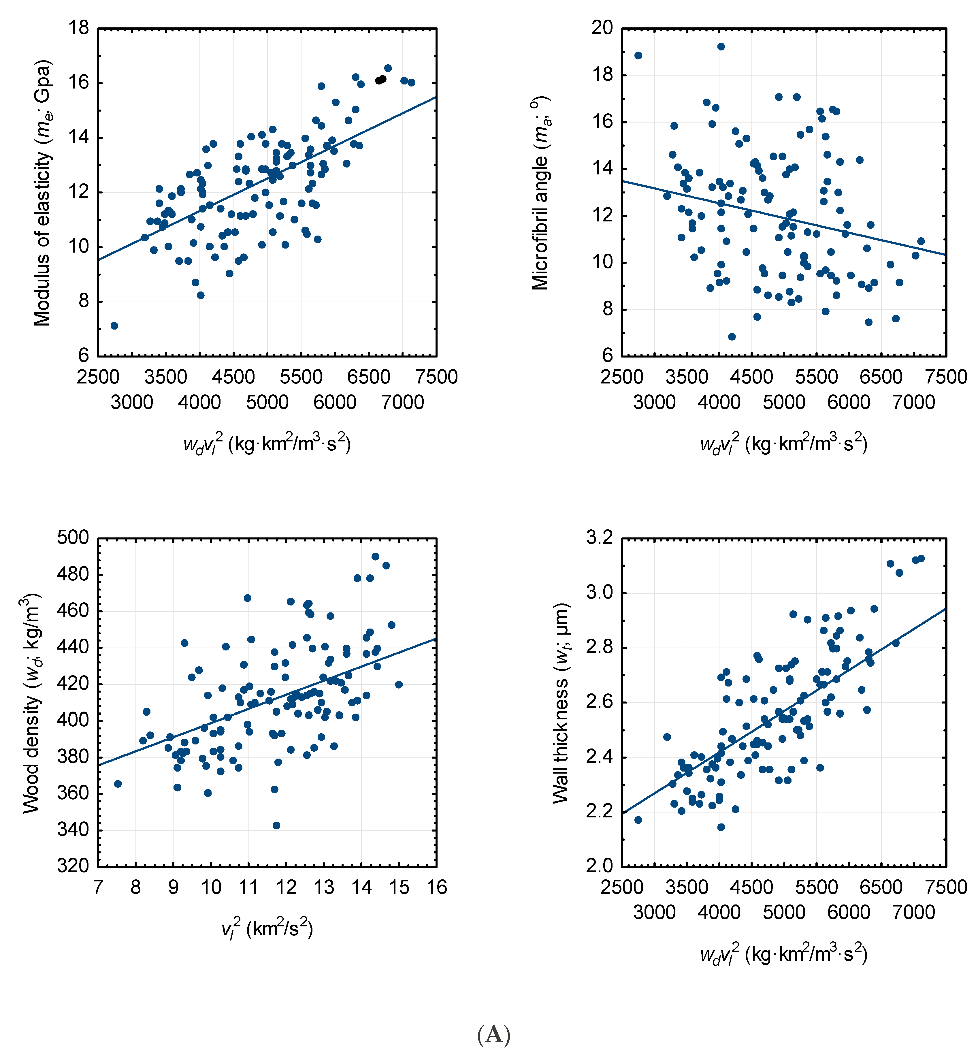
Figure 1. Scatterplots illustrating the relationship between each attribute and density-weighted and density-unweighted acoustic velocity ( v l ) for the jack pine logs within the calibration data subset: (A) m e = f ( w d v l 2 ) , w d = f ( v l 2 ) , m a = f ( w d v l 2 ) , and w t = f ( w d v l 2 ) relationships; and (B) d r = f ( w d v l 2 ) , d t = f ( w d v l 2 ) , and c o = f ( w d v l 2 ) and s a = f ( w d v l 2 ) relationships. The parameterized model is denoted by solid line (Table 7).
Forests 09 00749 g001aForests 09 00749 g001b
Figure 2. Scatterplots illustrating the relationship between each attribute and density-weighted and density-unweighted acoustic velocity ( v l ) for the jack pine logs within the validation data subset: (A) m e = f ( w d v l 2 ) , w d = f ( v l 2 ) , m a = f ( w d v l 2 ) , and w t = f ( w d v l 2 )   relationships; and (B) d r = f ( w d v l 2 ) , d t = f ( w d v l 2 ) , and c o = f ( w d v l 2 ) and s a = f ( w d v l 2 ) relationships. Note, where applicable, the superimposed parameterized model is denoted by solid line (Table 7) and superimposed contextual 95% prediction error limits are denoted by the parallel dashed lines.
Forests 09 00749 g002aForests 09 00749 g002b
Table 1. Product-based performance measures and their relationship with fiber attributes for boreal conifers.
Product CategoryPerformance MeasureRelationship with Fiber Attribute a
Biomass (e.g., pellets)Calorific value xylem density
Pulp and paper (e.g., paperboards, newsprint, facial tissues, and specialized coated papers)Tensile strength (tracheid wall thickness)−1, specific surface area
Tear strength fiber coarseness
Stretch microfibril angle
Bulk tracheid wall thickness, (tracheid diameter)−1
Light scattering (tracheid wall thickness)−1
Collapsibility tracheid wall thickness
Yield xylem density
Solid wood and composites (e.g., dimensional lumber; glulam-based beams)Strength xylem density, (microfibril angle)−1
Stiffness xylem density, modulus of elasticity, (microfibril angle)−1
Poles and squared timbers (e.g., utility poles and solid wood beams)Strength xylem density, (microfibril angle)−1
Stiffness xylem density, modulus of elasticity, (microfibril angle)−1
a Generic-based inferences derived from generalized end-product-specific performance metric—attribute relationships for boreal conifers (sensu [8]).
Table 2. Linear associations between the dynamic modulus of elasticity and other Silviscan-derived wood quality attributes for 3 boreal conifers and the resultant acoustic-based relationship inferred.
AttributeAssociation with Dynamic Modulus of Elasticity as Measured by the Pearson Product Moment Correlation Coefficient aStatistical InferenceEmpirical Linkage to Acoustic Velocity b
Black SpruceRed PineJack Pine
Wood density0.7765 *0.7585 *0.6717 * m e w d w d v l 2
Microfibril angle−0.8981 *−0.8075 *−0.7101 * m e m a 1 m a ( w d v l 2 ) 1
Tracheid wall thickness0.6765 *0.6871 *0.6648 * m e w t w t w d v l 2
Radial tracheid diameter−0.4477 *−0.3833 *−0.3169 * m e d r 1 d r ( w d v l 2 ) 1
Tangential tracheid diameter−0.3037 *−0.0886−0.0814 m e d t 1 d t ( w d v l 2 ) 1
Fiber coarseness0.20440.4385 *0.5412 * m e c o c o w d v l 2
Specific surface area−0.5812 *−0.6355 *−0.6368 * m e s a 1 s a ( w d v l 2 ) 1
a Species-specific bivariate linear associations between Silviscan-determined accumulative area-weighted mean fiber attributes as previously presented in Table 2 of Newton [16]: Pearson product moment correlation coefficient for the relationship between the dynamic modulus of elasticity and each attribute at breast-height (1.3 m) for 50 semi-mature black spruce trees [14], 54 mature red pine trees [16], and 61 semi-mature jack pine trees (this study) where * denotes a significant correlation at the 0.05 probability level. b Based on the primary m e w d v l 2 relationship for all attributes except wood density.
Table 3. Descriptive statistical summary of the mensuration characteristics of the 61 sample trees by site (n = 31 and 30 for Sewell and Tyrol, respectively).
VariableSiteMeanStandard ErrorMinimumMaximumCV a (%)
Diameter at breast-height (cm)Sewell18.82.1114.722.611.2
Tyrol24.42.1719.829.18.9
Breast-height age (year)Sewell500.9647511.9
Tyrol691.2766711.9
Total height (m)Sewell21.11.2618.322.96.0
Tyrol22.21.5719.524.67.1
Live crown ratio (%)Sewell26.14.5015.035.317.3
Tyrol28.27.2014.141.525.5
a Coefficient of variation.
Table 4. Descriptive statistical summary of the dimensions of the 243 sample logs and associated acoustic velocity measurements by log position (n = 243 of which 61, 61, 61 and 60 were first, second, third and fourth positioned logs, respectively).
VariableLog aMeanMedianStandard ErrorMinimumMaximumCV b (%)
Log length (m)1st4.304.360.043.485.007.7
2nd4.284.350.043.474.917.8
3rd4.284.370.043.184.917.9
4th4.254.370.062.274.8910.8
Mean log diameter (inside-bark; cm)1st19.4919.390.3513.7026.9214.1
2nd16.9717.030.3110.8921.7614.4
3rd14.3814.560.289.4119.2515.4
4th11.3010.990.267.5415.7117.5
Longitudinal stress wave velocity (vl; km/s)1st3.593.580.023.204.295.2
2nd3.593.620.033.154.325.5
3rd3.393.420.022.864.126.0
4th3.083.080.022.693.726.0
a Proceeding upwards from the stump to the stem apex, 1st, 2nd, 3rd and 4th denotes the ordinal position of the first, second, third and fourth log extracted from the main stem of the 61 jack pine sample trees. b Coefficient of variation.
Table 5. Descriptive statistical summary of the fiber attributes of by log position (n = 243 of which 61, 61, 61 and 60 were first, second, third and fourth positioned logs, respectively).
VariableLog aMeanMedianMinimumMaximumCV b (%)
Modulus of elasticity
(me; GPa)
1st12.7212.688.5916.7315.0
2nd12.8112.958.2416.1614.2
3rd12.3812.827.9315.8913.7
4th11.3311.577.1414.5712.7
Wood density
(wd; kg/m3)
1st430.38421.66372.88489.676.5
2nd416.48418.68337.88482.026.6
3rd407.47405.99359.76467.796.0
4th394.23391.66356.95442.255.1
Microfibril angle
(ma; °)
1st12.9812.797.4919.7121.1
2nd11.4710.956.3319.2322.7
3rd11.2510.926.2417.8422.6
4th12.5212.216.8420.2322.8
Tracheid wall thickness
(wt; µm)
1st2.702.672.353.167.6
2nd2.602.602.083.017.8
3rd2.522.492.222.927.3
4th2.392.372.172.775.9
Tracheid radial diameter
(dr; µm)
1st30.8030.9028.5133.003.7
2nd30.7530.9528.6932.743.5
3rd30.5230.6827.9932.793.7
4th30.0330.1826.4431.974.1
Tracheid tangential diameter
(dt; µm)
1st27.8727.9326.4129.882.4
2nd28.1328.1326.8930.252.5
3rd28.1028.1626.5329.722.5
4th27.9727.9926.3829.632.6
Fiber coarseness
(co; µg/m)
1st406.02406.67360.44471.206.8
2nd395.23394.97339.39447.857.1
3rd383.33383.76328.30455.347.2
4th364.51365.10311.38420.686.3
Specific surface area
(sa; m2/kg)
1st314.32315.76275.59351.466.4
2nd322.71321.31284.37372.466.4
3rd328.16327.71287.81366.306.4
4th338.15341.99297.17369.335.0
a Proceeding upwards from the stump to the stem apex, 1st, 2nd, 3rd and 4th denotes the ordinal position of the first, second, third and fourth log extracted from the main stem of the 61 jack pine sample trees. b Coefficient of variation.
Table 6. Descriptive statistical summary of the calibration (n = 122 logs) and validation (n = 121 logs) data subsets.
VariableData SubsetMeanMinimumMaximumCV a (%)
Longitudinal stress wave velocity (vl; km/s)Calibration3.422.744.327.8
Validation3.412.694.298.8
Modulus of elasticity (me; GPa)Calibration12.287.1416.5714.8
Validation12.347.9316.7314.7
Wood density (wd; kg/m3)Calibration412.41343.02489.676.9
Validation412.02337.88482.026.8
Microfibril angle (ma; °)Calibration12.106.8419.2321.7
Validation12.016.2420.2324.3
Tracheid wall thickness (wt; µm)Calibration2.562.143.138.6
Validation2.552.083.168.3
Tracheid radial diameter (dr; µm)Calibration30.5927.9933.003.8
Validation30.4726.4432.743.9
Tracheid tangential diameter (dt; µm)Calibration28.0126.4129.882.5
Validation28.0226.3830.252.5
Coarseness (co; µg/m)Calibration388.35318.32459.908.1
Validation386.38311.38471.207.7
Specific surface area (sa; m2/kg)Calibration325.22278.70369.906.8
Validation326.36275.59372.466.4
a Coefficient of variation.
Table 7. Attribute-specific regression results for the mixed-effects model specification (Equation (5)): parameter estimates, regression statistics and compliance indicators.
RelationshipParameter Estimates aRegression Statistics and Compliance Indices
γ ^ 0 γ ^ 1 Degrees of Freedom b (nreg, nres)I2cRandom Effects dHomogeneity of Variance eSpatial Correlation f
m e w d v l 2 6.54390.0011941, 1200.466*H0H0
w d v l 2 321.64837.72011, 1200.315*H0H0
m a w d v l 2 15.0699−0.000631, 1200.079*H0H0
w t w d v l 2 1.81900.0001501, 1200.603*H0H0
d r w d v l 2 30.6445−0.000037ns1, 120----
d t w d v l 2 28.2502−0.000048ns1, 120----
c o w d v l 2 300.02000.0177901, 1200.456*H0H0
s a w d v l 2 388.1280−0.0127241, 1200.497*H0H0
a γ ^ 0 is a random effect intercept parameter estimate specific to the kth attribute and γ ^ 1 is fixed effect slope parameter estimate specific to the kth attribute. Note, parameter estimates not significantly (p > 0.05) different from zero are superscripted by ns. b Degrees of freedom for regression (nreg) and residual error (nres). c I2 is the index-of-fit squared (Equation (6)). d Non-significant (p > 0.05) and significant (p ≤ 0.05) random effects are denoted ns and *, respectively (i.e., testing the null hypothesis that u 0 = 0 versus the alternative hypothesis u 0 ≠ 0 in Equation (5)). e Non-rejection and rejection of the constant variance assumption at the 0.01 probability level are denoted H0 and H1, respectively, as determined from Park’s test for homoscedasticity (see text for details). f Non-rejection and rejection of the independence assumption (spatially uncorrelated residuals) at the 0.01 probability level are denoted H0 and H1, respectively, as determined from the residual regression approach ([30]; see text for details).
Table 8. Evaluation metrics for the parameterized models: goodness-of-fit, lack-of-fit statistics and predictive ability metrics.
RelationshipGoodness-of-fit StatisticLack-of-fit MeasuresPredictive Ability: 95% Error Intervals d
Hypotheses bAbsolute cRelative c (%)PredictionTolerance
I2a α 0 = 0 α 1 = 1 Mean Bias95% CLMean Bias95% CLAbsoluteRelative (%)AbsoluteRelative (%)
95% CL95% CL95% CL95% CL
m e w d v l 2 0.526H0H0−0.031±0.2260.986±2.049±2.489±22.543±2.759±24.993
w d v l 2 0.304H0H0−0.125±4.2320.292±1.028±46.550±11.306±51.610±12.535
m a w d v l 2 0.075H0H00.050±0.5065.998 *±4.553±5.565±50.087±6.170±55.531
w t w d v l 2 0.583H0H00.004±0.0250.151±0.971±0.272±10.679±0.301±11.840
c o w d v l 2 0.426H0H0−0.399±4.0820.250±1.070±44.903±11.764±49.784±13.043
s a w d v l 2 0.438H0H00.224±2.8120.305±0.861±30.937±9.468±34.299±10.497
aI2 is the index-of-fit squared (Equation (6)). b Testing the (1) null hypothesis that α 0 = 0 versus the alternative hypothesis α 0 0 where H0 and H1 denote the non-rejection and rejection of the null hypothesis at the 0.05 probability level, and (2) null hypothesis that α 1 = 1 versus the alternative hypothesis α 1 1 where H0 and H1 denote the non-rejection and rejection of the null hypothesis at the 0.05 probability level, where α 0 and α 1 are derived from the simple linear ordinary least squares regression relationship between observed (y) and predicted (x) values ( y = α 0 + α 1 x + ε where ε is an error term [31]). c Mean absolute (Equation (7)) and relative (Equation (8)) bias and the limits (CL) of the associated 95% confidence interval (Equation (9)) where mean values not significantly (p > 0.05) different from zero were indicative of an unbiased relationship (i.e., mean bias ± 95% confidence limits (CL)); note, underlined CL values denote approximations given the presence of significant (p ≤ 0.05) non-normality within the underlying error distribution; absolute error units are attribute-specific: GPa, kg/m3, µm, µg/m and m2/kg for me, wd, ma, wt, co and sa, respectively. d CL for the 95% prediction and tolerance error intervals for absolute and relative errors (Equations (10) and (11), respectively): mean bias ± 95% CL; specifically, there is a 95% probability that a future error will be within the stated prediction interval and that there is a 95% probability that 95% of all future errors will be within the stated tolerance interval [32,33]; note, underlined CL values denote approximations given the presence of significant (p ≤ 0.05) non-normality within the underlying error distribution.
Table 9. Predictive performance of parameterized models when deploying acoustic-based wood density estimates.
RelationshipLack-of-fit Measures aPredictive Ability: 95% Error Intervals b
AbsoluteRelative (%)Prediction (Stand-Level)Tolerance
Mean95% CL eMean95% CLAbsoluteRelative (%)Absolute bRelative (%)
bias bias 95% CL95% CL95% CL95% CL
m e w d v l 2 −0.033±0.2511.118±2.240±2.756±24.640±3.055±27.318
(±0.562)5.028)
m a w d v l 2 0.051±0.5056.000 *±4.522±5.554±49.738±6.158±55.144
(±1.129)(±10.111)
w t w d v l 2 −0.004±0.0250.151±0.971±0.272±10.679±0.301±11.840
(±0.055)(±2.171)
c o w d v l 2 −0.440±4.6710.300±1.219±51.383±13.406±56.968±14.863
(±10.445)(±2.725)
s a w d v l 2 0.253±3.3400.369±1.027±36.734±11.291±40.727±12.519
(±7.467)(±2.295)
a Mean absolute (Equation (7)) and relative (Equation (8)) bias and the limits (CL) of the associated 95% confidence interval (Equation (9)) where mean values not significantly (p > 0.05) different from zero were indicative of an unbiased relationship; note, underlined CL values denote approximations given the presence of significant (p ≤ 0.05) non-normality within the underlying error distribution; absolute error units are attribute-specific: GPa, °, µm, µg/m and m2/kg for me, ma, wt, co and sa, respectively; and * denotes significant bias. b Confidence limits for the 95% prediction and tolerance error intervals for absolute and relative errors (Equations (10) and (11), respectively): mean bias ± 95% CL; specifically, there is a 95% probability that a future error will be within the stated prediction interval and that there is a 95% probability that 95% of all future errors will be within the stated tolerance interval (sensu [32]); notes, (1) absolute error units are attribute-specific as stated above, (2) underlined CL values denote approximations given the presence of significant (p ≤ 0.05) non-normality within the underlying error distribution, and (3) stand-level CL intervals denote the 95% prediction limits for the mean error generated when group sampling (e.g., assigning a mean attribute estimate to 30-log sample (pile) derived from a single stand).