
CAT-Site: Predicting Protein Binding Sites Using a Convolutional Neural Network


Abstract

1. Introduction
1.1. Related Work
1.2. Aim and Contributions of This Work
- A data preprocessing method and novel method for alignment of aminoacid sequences and their clustering;
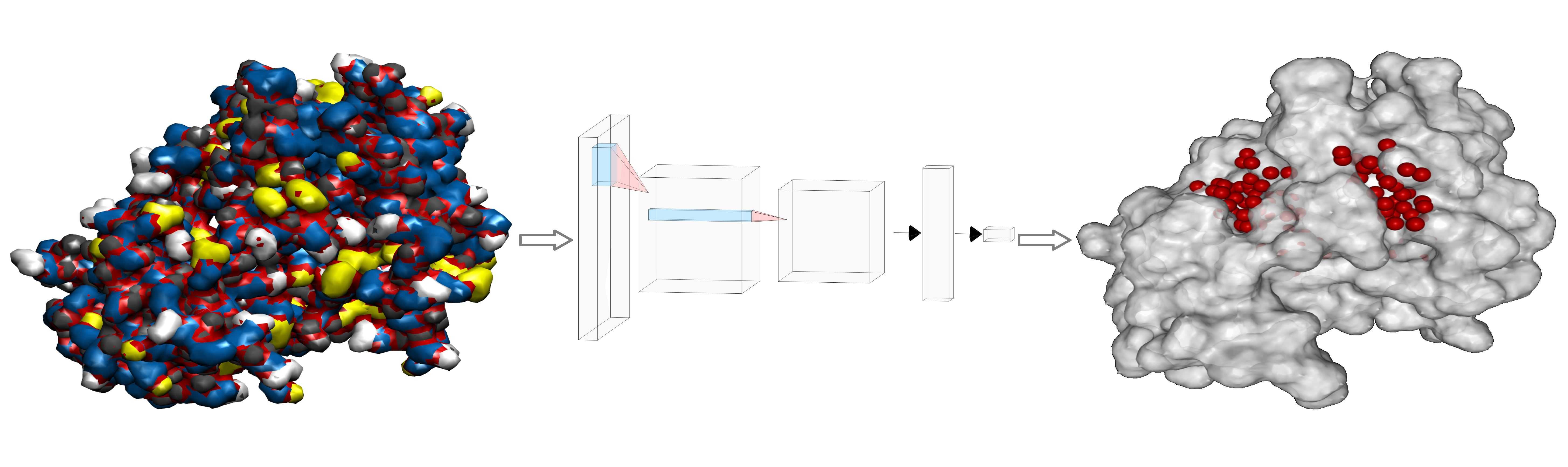
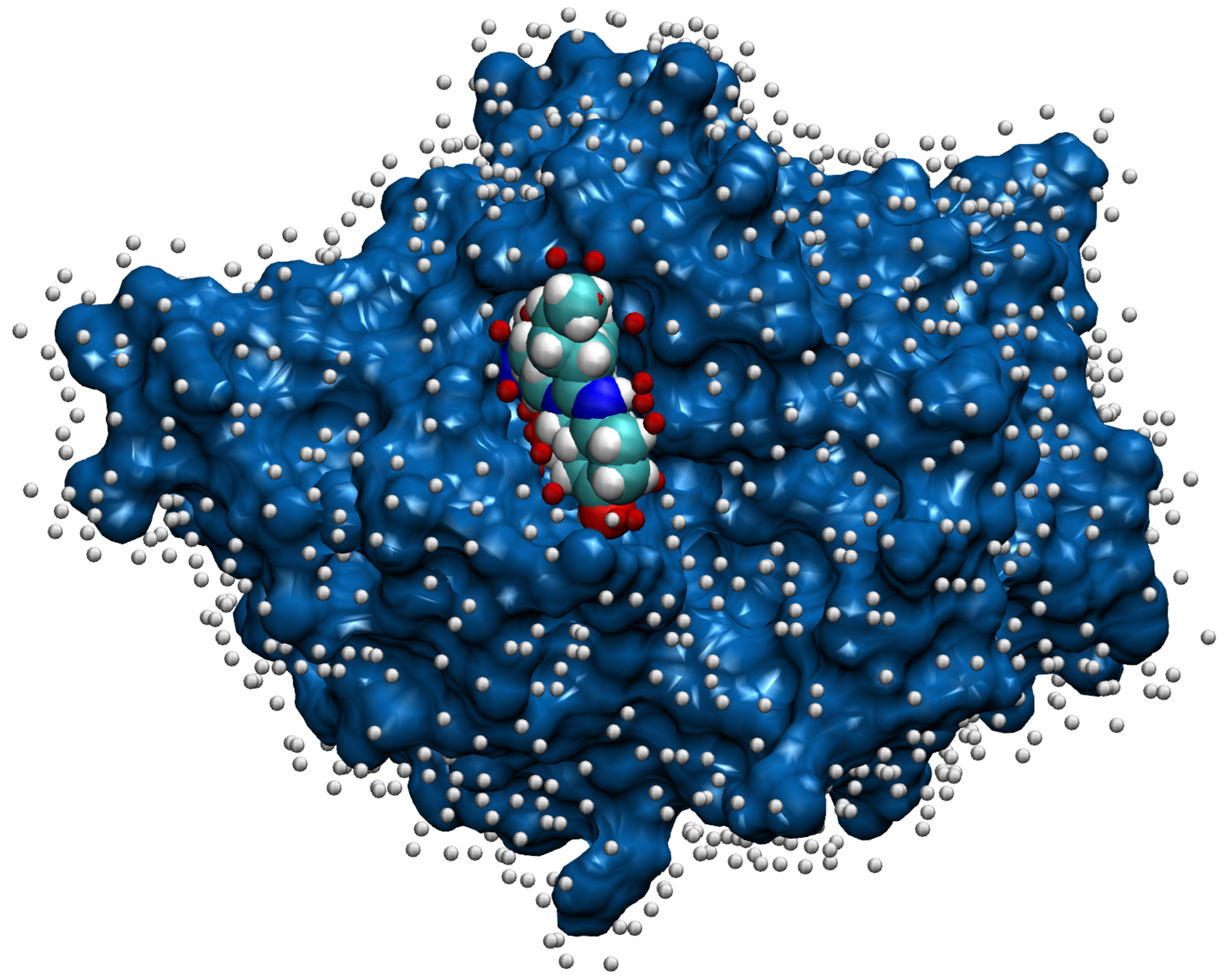
- Representation of molecules for machine learning and modeling them with a CNN that receives the three-dimensional images with eight channels as its input;
- The novel method for final combining of ligandability predictions into binding sites by processing the output of the CNN.
2. Materials and Methods
2.1. Selection and Preparation of Training Data
2.2. Alignment of Amino Acid Sequences and Their Clustering
2.3. Merging of Ligands of Similar Chains
- We read and sort the chains from the cluster in descending order based on the number of bound ligands and the total number of atoms of bound ligands. Sorting by these two criteria, we prioritize chains with more bound ligands, and in case two chains have the same number of ligands, we prioritize the chain with larger ligands on average. The reason for the second sorting criterion is that ligands bound to approximately the same binding site can be significantly different in size. If in such a case we chose the smaller ligand as the representative occupant of the binding site, a large part of the actual binding site would be falsely marked as non-ligandable.
- We choose the representative chain based on the number of chains from the cluster to which it can be aligned well. The basic idea is to find a chain from the cluster that can be aligned to a sufficient number of other chains in its cluster. We follow the order in the sorted list of chains described in the previous step until we find a chain that fits our criteria. The search for the common orientation of chains is done by adapting the method prody_align from the ProDy library [27]. This method receives as an input a reference chain and a list of chains that we wish to rotate and translate so they align with the reference chain. The algorithm also takes the lower bound for sequence similarity seqid=0.9 and the lower bound for covering overlap=0.9, which correspond to the parameters and from Section 2.2.
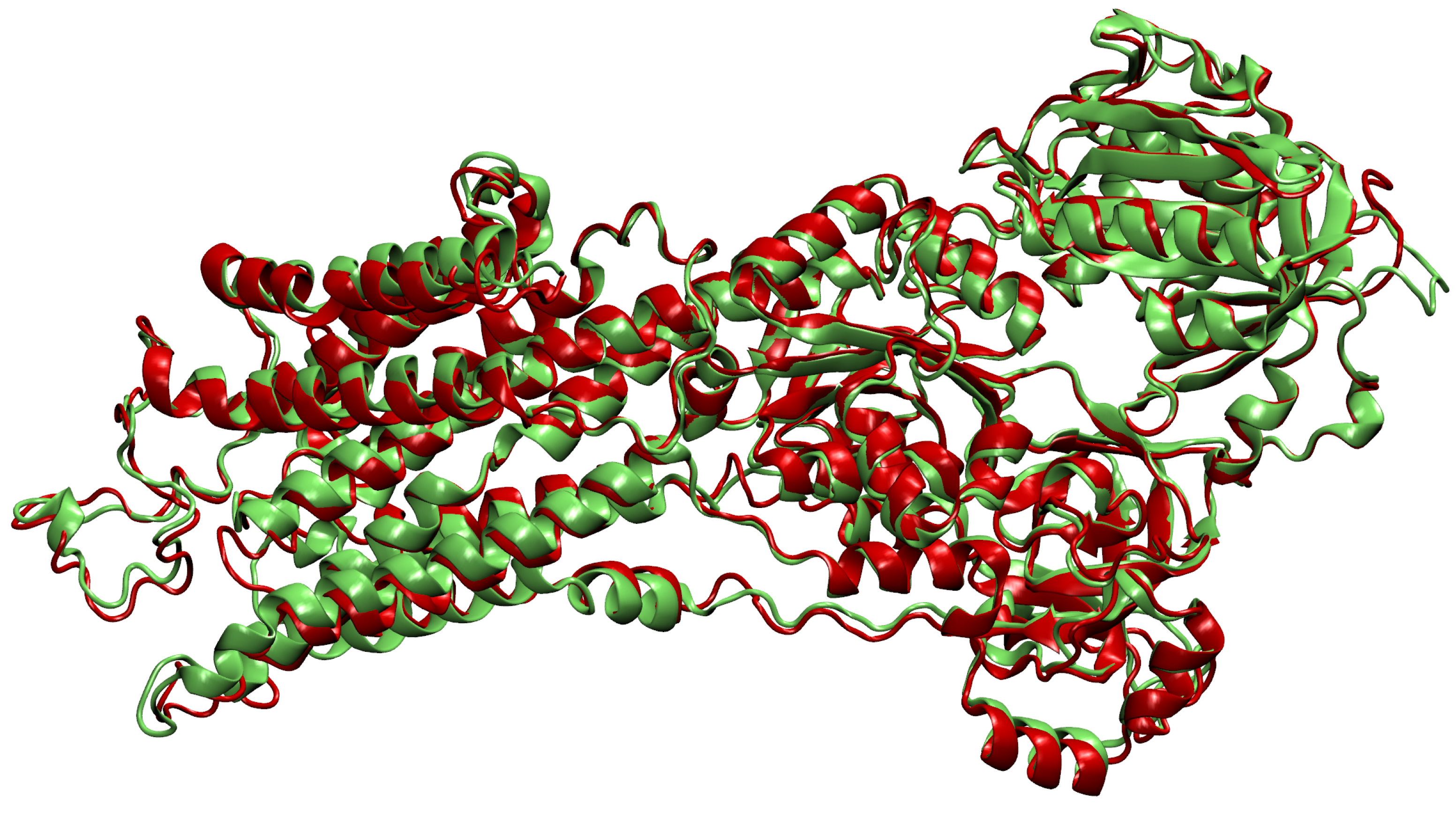
- Then, we add ligands to the selected reference chain from sufficiently similar chains. We only add ligands that do not intersect with the ligands already bound to the reference chain. We also discard ligands that intersect with the reference chain or are too far away. In this part, we consider two chains as sufficiently similar if the root mean square deviation of pairs of the matching C atoms is smaller than 2 Å. That is,where and are lists of matching C atoms, , and is the euclidean distance between two points. The upper bound of 2 was set empirically, taking into account the alignment or oriented pairs of chains. An example where Å is shown in Figure 3. The chains align sufficiently well despite the value being close to the upper bound.
- If we were not able to align all chains in the cluster to a single reference chain, we repeat the process on the remaining chains—we assign the remaining chains to the new cluster and go back to the first step.
2.4. Representation of Molecules for Machine Learning
2.5. Machine Learning with Convolutional Neural Network
2.6. Combining Ligandability Predictions into Binding Sites
- Number of points;
- Average distance of points from the geometric center;
- Standard deviation of distance of points from the geometric center.
| Algorithm 1 Grouping predicted ligandable points into binding sites. |
| 1: function binding_sites() |
| 2: ▹ Real values a and b define the interval in which we look for the best c value. |
| 3: |
| 4: ▹ Real value c is the threshold for classification of ligandability predictions in each iteration of the while loop. |
| 5: select_ligandable_points() |
| 6: |
| 7: |
| 8: |
| 9: while is not “break” do |
| 10: components() |
| 11: for do |
| 12: if properties fit into quantile bounds then |
| 13: append to |
| 14: end if |
| 15: end for |
| 16: |
| 17: if is “increase a” then |
| 18: |
| 19: else if is “decrease b” then |
| 20: |
| 21: end if |
| 22: |
| 23: |
| 24: select_ligandable_points() |
| 25: compute_condition() |
| 26: end while |
| 27: return |
| 28: end function |
| 29: function compute_condition() |
| 30: if then return “break” |
| 31: else if then return “increase a” |
| 32: else if is an then return “decrease b” |
| 33: else if then return “decrease b” |
| 34: else if then return “increase a” |
| 35: else if then return “decrease b” |
| 36: else if then return “increase a” |
| 37: else if then return “decrease b” |
| 38: else if then return “increase a” |
| 39: else |
| 40: return “decrease b” |
| 41: end if |
| 42: end function |
| 43: function components() |
| 44: |
| 45: ▹ Two points are connected if they are closer than 4Å |
| 46: ▹ Create a graph with vertices V and edges E |
| 47: return connected_components(G) |
| 48: end function |
| 49: function select_ligandable_points() |
| 50: |
| 51: for do |
| 52: if then ▹ Check if prediction for is higher than threshold c |
| 53: append to |
| 54: end if |
| 55: end for |
| 56: return |
| 57: end function |
3. Results
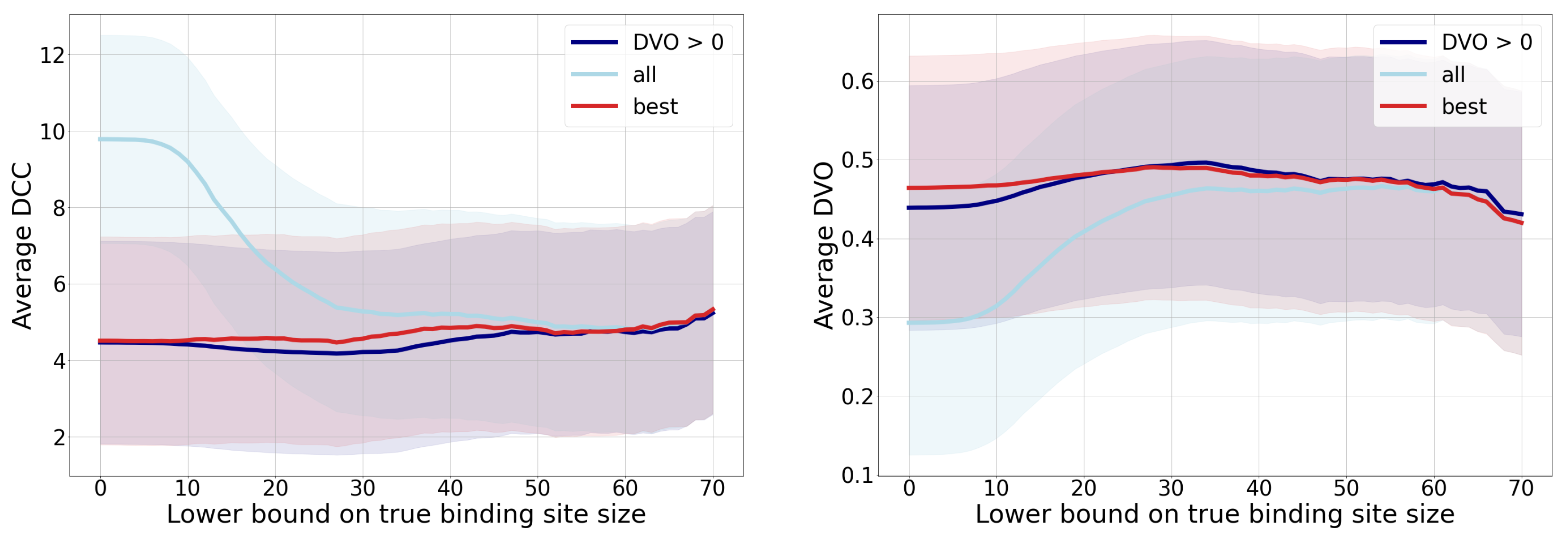
3.1. Distance from the Center and Discrete Volumetric Overlap
3.2. Classification Performance Metrics
4. Discussion
- The histogram of sensitivity and recall shows that a smaller-threshold t results in more ligandable points. A ratio of predicted true ligandable points is therefore higher with a smaller t, while the higher t could result in overlooking some of the possible binding sites.
- A higher-threshold t on the histogram of specificity results in a higher number of non-ligandable points. The ratio of predicted true non-ligandable points (i.e., specificity) is therefore higher with higher values of t.
- The precision metric reports a ratio of predicted ligandable points that are truly ligandable. A smaller-threshold t here indicates worse results; namely, it causes a larger number of false positive points to be predicted. Similarly, a higher t causes a smaller number of predicted true ligandable points; hence, the precision remains low.
- The histogram of the loss function is independent of changing the threshold t since its value is computed directly from the predicted value for each individual point.
- The histogram of accuracy reveals influence of the imbalanced data set. A higher-threshold t here causes only a few points to be predicted as ligandable, but as the number of non-ligandable points is high, the resulting accuracy is also high. As the simple solution, we also compute the balanced accuracy that is computed as an average of sensitivity and specificity. Their graphs show that the balanced accuracy is low in some parts due to the low sensitivity for some chains. Here, a higher-threshold t also causes lower sensitivity.
- The -score is a harmonic mean between precision and sensitivity. Higher values of -score mean that both underlying measures are high; while low values can be a result of either one of them being low. If we observe the threshold , we can note the high sensitivity and the low precision, resulting in a low -score. We can also note the best ratio with , where the sensitivity is moderate and the precision seems to be the highest.
- Matthews correlation coefficient is a number from the interval that expresses how well model’s predictions are correlated with true values. Values higher than 0 denote positive correlation, and values less than 0 denote negative correlation. A higher value denotes higher predictive capability. We can see from the graph that the best results are achieved with a threshold , as the correlation is lower with all the remaining thresholds.
5. Conclusions
Author Contributions
Funding
Institutional Review Board Statement
Informed Consent Statement
Data Availability Statement
Acknowledgments
Conflicts of Interest
Abbreviations
| CNN | Convolutional Neural Network |
| SAS | Solvent Accessible Surface |
| DVO | Discrete Volumetric Overlap |
| DCC | Distance from Center to Center |
| MCC | Matthews Correlation Coefficient |
| PDB | Protein Data Bank |
References
- Workman, P.; Draetta, G.F.; Schellens, J.H.; Bernards, R. How Much Longer Will We Put Up With 100,000 Cancer Drugs? Cell 2017, 168, 579–583. [Google Scholar] [CrossRef] [PubMed]
- Naqvi, A.A.; Mohammad, T.; Hasan, G.M.; Hassan, M.; Hassan, M.I. Advancements in docking and molecular dynamics simulations towards ligand-receptor interactions and structure-function relationships. Curr. Top. Med. Chem. 2018, 18, 1755–1768. [Google Scholar] [CrossRef] [PubMed]
- Pinzi, L.; Rastelli, G. Molecular Docking: Shifting Paradigms in Drug Discovery. Int. J. Mol. Sci. 2019, 20, 4331. [Google Scholar] [CrossRef]
- Meng, X.Y.; Zhang, H.X.; Mezei, M.; Cui, M. Molecular docking: A powerful approach for structure-based drug discovery. Curr. Comput.-Aided Drug Des. 2011, 7, 146–157. [Google Scholar] [CrossRef] [PubMed]
- Gupta, M.; Sharma, R.; Kumar, A. Docking techniques in pharmacology: How much promising? Comput. Biol. Chem. 2018, 76, 210–217. [Google Scholar] [CrossRef]
- Campillos, M.; Kuhn, M.; Gavin, A.C.; Jensen, L.J.; Bork, P. Drug Target Identification Using Side-Effect Similarity. Science 2008, 321, 263–266. [Google Scholar] [CrossRef]
- Torres, P.H.M.; Sodero, A.C.R.; Jofily, P.; Silva-Jr, F.P. Key Topics in Molecular Docking for Drug Design. Int. J. Mol. Sci. 2019, 20, 4574. [Google Scholar] [CrossRef]
- Salmaso, V.; Moro, S. Bridging Molecular Docking to Molecular Dynamics in Exploring Ligand-Protein Recognition Process: An Overview. Front. Pharmacol. 2018, 9, 923. [Google Scholar] [CrossRef]
- Macari, G.; Toti, D.; Polticelli, F. Computational methods and tools for binding site recognition between proteins and small molecules: From classical geometrical approaches to modern machine learning strategies. J. Comput.-Aided Mol. Des. 2019, 33, 887–903. [Google Scholar] [CrossRef]
- Crampon, K.; Giorkallos, A.; Deldossi, M.; Baud, S.; Steffenel, L.A. Machine-learning methods for ligand–protein molecular docking. Drug Discov. Today 2022, 27, 151–164. [Google Scholar] [CrossRef]
- Guilloux, V.L.; Schmidtke, P.; Tuffery, P. Fpocket: An open source platform for ligand pocket detection. BMC Bioinform. 2009, 10, 168. [Google Scholar] [CrossRef] [PubMed]
- Krivák, R.; Hoksza, D. P2Rank: Machine learning based tool for rapid and accurate prediction of ligand binding sites from protein structure. J. Cheminform. 2018, 10, 39. [Google Scholar] [CrossRef] [PubMed]
- Krivák, R.; Hoksza, D. Improving protein-ligand binding site prediction accuracy by classification of inner pocket points using local features. J. Cheminform. 2015, 7, 12. [Google Scholar] [CrossRef] [PubMed]
- Jiménez, J.; Doerr, S.; Martínez-Rosell, G.; Rose, A.S.; Fabritiis, G.D. DeepSite: Protein-binding site predictor using 3D-convolutional neural networks. Bioinformatics 2017, 33, 3036–3042. [Google Scholar] [CrossRef] [PubMed]
- Aggarwal, R.; Gupta, A.; Chelur, V.; Jawahar, C.V.; Priyakumar, U.D. DeepPocket: Ligand Binding Site Detection and Segmentation using 3D Convolutional Neural Networks. J. Chem. Inf. Model. 2021, 62, 5069–5079. [Google Scholar] [CrossRef]
- Sunseri, J.; Koes, D.R. libmolgrid: Graphics Processing Unit Accelerated Molecular Gridding for Deep Learning Applications. J. Chem. Inf. Model. 2020, 60, 1079–1084. [Google Scholar] [CrossRef]
- Ronneberger, O.; Fischer, P.; Brox, T. U-Net: Convolutional Networks for Biomedical Image Segmentation; Springer: Cham, Switzerland, 2015; pp. 234–241. [Google Scholar] [CrossRef]
- Selvaraju, R.R.; Cogswell, M.; Das, A.; Vedantam, R.; Parikh, D.; Batra, D. Grad-CAM: Visual Explanations from Deep Networks via Gradient-Based Localization. Int. J. Comput. Vis. 2019, 128, 336–359. [Google Scholar] [CrossRef]
- Wang, R.; Fang, X.; Lu, Y.; Yang, C.Y.; Wang, S. The PDBbind database: Methodologies and updates. J. Med. Chem. 2005, 48, 4111–4119. [Google Scholar] [CrossRef]
- Desaphy, J.; Bret, G.; Rognan, D.; Kellenberger, E. sc-PDB: A 3D-database of ligandable binding sites—10 years on. Nucleic Acids Res. 2014, 43, D399–D404. [Google Scholar] [CrossRef]
- Berman, H.M.; Westbrook, J.; Feng, Z.; Gilliland, G.; Bhat, T.N.; Weissig, H.; Shindyalov, I.N.; Bourne, P.E. The Protein Data Bank. Nucleic Acids Res. 2000, 28, 235–242. [Google Scholar] [CrossRef]
- Steinegger, M.; Söding, J. MMseqs2 enables sensitive protein sequence searching for the analysis of massive data sets. Nat. Biotechnol. 2017, 35, 1026–1028. [Google Scholar] [CrossRef] [PubMed]
- Smith, T.; Waterman, M. Identification of common molecular subsequences. J. Mol. Biol. 1981, 147, 195–197. [Google Scholar] [CrossRef] [PubMed]
- Volkers, G.; Damas, J.M.; Palm, G.J.; Panjikar, S.; Soares, C.M.; Hinrichs, W. Putative dioxygen-binding sites and recognition of tigecycline and minocycline in the tetracycline-degrading monooxygenase TetX. Acta Crystallogr. Sect. D Biol. Crystallogr. 2013, 69, 1758–1767. [Google Scholar] [CrossRef]
- Volkers, G.; Palm, G.; Weiss, M.; Hinrichs, W. Structure of the Tetracycline Degrading Monooxygenase Tetx in Complex With Minocycline; International Union of Crystallography: Chester, UK, 2012. [Google Scholar] [CrossRef]
- Humphrey, W.; Dalke, A.; Schulten, K. VMD: Visual molecular dynamics. J. Mol. Graph. 1996, 14, 33–38. [Google Scholar] [CrossRef]
- Bakan, A.; Meireles, L.M.; Bahar, I. ProDy: Protein Dynamics Inferred from Theory and Experiments. Bioinformatics 2011, 27, 1575–1577. [Google Scholar] [CrossRef]
- Takahashi, M.; Kondou, Y.; Toyoshima, C. Interdomain communication in calcium pump as revealed in the crystal structures with transmembrane inhibitors. Proc. Natl. Acad. Sci. USA 2007, 104, 5800–5805. [Google Scholar] [CrossRef] [PubMed]
- Takahashi, M.; Kondou, Y.; Toyoshima, C. Crystal structure of the SR CA2+-ATPASE with bound CPA and TG. 2007. [Google Scholar] [CrossRef]
- Takahashi, M.; Kondou, Y.; Toyoshima, C. Crystal structure of the SR CA2+-ATPASE with bound CPA in the presence of curcumin. 2007. [Google Scholar] [CrossRef]
- Doerr, S.; Harvey, M.J.; Noé, F.; De Fabritiis, G. HTMD: High-Throughput Molecular Dynamics for Molecular Discovery. J. Chem. Theory Comput. 2016, 12, 1845–1852. [Google Scholar] [CrossRef] [PubMed]
- Lee, B.; Richards, F. The interpretation of protein structures: Estimation of static accessibility. J. Mol. Biol. 1971, 55, 379-IN4. [Google Scholar] [CrossRef] [PubMed]
- Willighagen, E.L.; Mayfield, J.W.; Alvarsson, J.; Berg, A.; Carlsson, L.; Jeliazkova, N.; Kuhn, S.; Pluskal, T.; Rojas-Chertó, M.; Spjuth, O.; et al. Erratum to: The Chemistry Development Kit (CDK) v2.0: Atom typing, depiction, molecular formulas, and substructure searching. J. Cheminform. 2017, 9, 33. [Google Scholar] [CrossRef]
- Toney, J.H.; Fitzgerald, P.M.; Grover-Sharma, N.; Olson, S.H.; May, W.J.; Sundelof, J.G.; Vanderwall, D.E.; Cleary, K.A.; Grant, S.K.; Wu, J.K.; et al. Antibiotic sensitization using biphenyl tetrazoles as potent inhibitors of Bacteroides fragilis metallo-β-lactamase. Chem. Biol. 1998, 5, 185–196. [Google Scholar] [CrossRef]
- Fitzgerald, P.; Toney, J.; Grover, N.; Vanderwall, D. METALLO-BETA-LACTAMASE IN COMPLEX WITH L-159, 061, 1998. [CrossRef]
- O’Boyle, N.M.; Banck, M.; James, C.A.; Morley, C.; Vandermeersch, T.; Hutchison, G.R. Open Babel: An open chemical toolbox. J. Cheminform. 2011, 3, 33. [Google Scholar] [CrossRef] [PubMed]
- Paszke, A.; Gross, S.; Massa, F.; Lerer, A.; Bradbury, J.; Chanan, G.; Killeen, T.; Lin, Z.; Gimelshein, N.; Antiga, L.; et al. PyTorch: An Imperative Style, High-Performance Deep Learning Library. In Proceedings of the 33rd International Conference on Neural Information Processing Systems, Vancouver, BC, Canada, 8–14 December 2019; Curran Associates Inc.: Red Hook, NY, USA, 2019. [Google Scholar]
- Smith, L.N.; Topin, N. Super-Convergence: Very Fast Training of Neural Networks Using Large Learning Rates. arXiv 2017, arXiv:1708.07120. [Google Scholar] [CrossRef]
- Yang, H.; Wang, Z.; Shen, Y.; Wang, P.; Jia, X.; Zhao, L.; Zhou, P.; Gong, R.; Li, Z.; Yang, Y.; et al. Crystal Structure of the Nosiheptide-Resistance Methyltransferase of Streptomyces actuosus. Biochemistry 2010, 49, 6440–6450. [Google Scholar] [CrossRef] [PubMed]
- Yang, H.; Wang, Z.; Shen, Y.; Wang, P.; Murchie, A.; Xu, Y. Structure of the Nosiheptide-resistance methyltransferase S-adenosyl-L-methionine Complex. Biochemistry 2010, 49, 6440–6450. [Google Scholar] [CrossRef]
- Ahmad, S.; Muthukumar, S.; Kuncha, S.K.; Routh, S.B.; Yerabham, A.S.; Hussain, T.; Kamarthapu, V.; Kruparani, S.P.; Sankaranarayanan, R. Specificity and catalysis hardwired at the RNA—Protein interface in a translational proofreading enzyme. Nat. Commun. 2015, 6, 7552. [Google Scholar] [CrossRef]
- Ahmad, S.; Yerabham, A.; Kamarthapu, V.; Sankaranarayanan, R. Editing domain of threonyl-tRNA synthetase from Methanococcus jannaschii with L-Thr3AA. 2015. [Google Scholar] [CrossRef]
- Heinrich, T.; Grädler, U.; Böttcher, H.; Blaukat, A.; Shutes, A. Allosteric IGF-1R Inhibitors. ACS Med. Chem. Lett. 2010, 1, 199–203. [Google Scholar] [CrossRef]
- Graedler, U.; Heinrich, T.; Boettcher, H.; Blaukat, A.; Shutes, A.; Askew, B. IGF-1RK in complex with ligand MSC1609119A-1. 2010. [CrossRef]
- Dock-Bregeon, A.C.; Rees, B.; Torres-Larios, A.; Bey, G.; Caillet, J.; Moras, D. Achieving Error-Free Translation. Mol. Cell 2004, 16, 375–386. [Google Scholar] [CrossRef]
- Dock-Bregeon, A.; Rees, B.; Torres-Larios, A.; Bey, G.; Caillet, J.; Moras, D. Crystal structure of the editing domain of threonyl-tRNA synthetase complexed with an analog of seryladenylate. 2004. [Google Scholar] [CrossRef]


| Atom Type | Description |
|---|---|
| C | Non H-bonding aliphatic carbon |
| A | Non H-bonding aromatic carbon |
| NA | Nitrogen, one H-bond acceptor |
| NS | Nitrogen acceptor of NS type |
| OA | Oxygen, two H-bonds acceptor |
| OS | Oxygen acceptor of type OS |
| SA | Sulfur, two H-bonds acceptor |
| HD | Hydrogen, donor of one H-bond |
| HS | Hydrogen, donor of HS type |
| MG | Magnesium, not binding to hydrogen |
| ZN | Zinc, not binding to hydrogen |
| MN | Manganese, not binding to hydrogen |
| CA | Calcium, not binding to hydrogen |
| FE | Iron, not binding to hydrogen |
| Property | Examples |
|---|---|
| hydrophobicity | atoms of type C or A |
| aromaticity | atoms of type A |
| H-bond acceptors | atoms of type NA, or NS, or OA, or OS, or SA |
| H-bond donor | atoms of type HD, or HS partnering with O or N |
| positive ionizability | positively charged atoms |
| negative ionizability | negatively charged atoms |
| metal | atoms of type MG, or ZN, or MN, or CA, or FE |
| excluded volume | all atom types (including the ones not given in Table 1) |
| Metric\Group | All | All > 30 | Best | DVO > 0 |
|---|---|---|---|---|
| distance | ||||
| DVO | ||||
| Threshold t | 0.3 | 0.5 | 0.7 | 0.9 |
|---|---|---|---|---|
| sensitivity | ||||
| specificity | ||||
| precision | ||||
| loss function | ||||
| accuracy | ||||
| balanced acc. | ||||
| -score | ||||
| MCC |
Disclaimer/Publisher’s Note: The statements, opinions and data contained in all publications are solely those of the individual author(s) and contributor(s) and not of MDPI and/or the editor(s). MDPI and/or the editor(s) disclaim responsibility for any injury to people or property resulting from any ideas, methods, instructions or products referred to in the content. |
© 2022 by the authors. Licensee MDPI, Basel, Switzerland. This article is an open access article distributed under the terms and conditions of the Creative Commons Attribution (CC BY) license (https://creativecommons.org/licenses/by/4.0/).
Share and Cite
Petrovski, Ž.H.; Hribar-Lee, B.; Bosnić, Z. CAT-Site: Predicting Protein Binding Sites Using a Convolutional Neural Network. Pharmaceutics 2023, 15, 119. https://doi.org/10.3390/pharmaceutics15010119
Petrovski ŽH, Hribar-Lee B, Bosnić Z. CAT-Site: Predicting Protein Binding Sites Using a Convolutional Neural Network. Pharmaceutics. 2023; 15(1):119. https://doi.org/10.3390/pharmaceutics15010119
Chicago/Turabian StylePetrovski, Žan Hafner, Barbara Hribar-Lee, and Zoran Bosnić. 2023. "CAT-Site: Predicting Protein Binding Sites Using a Convolutional Neural Network" Pharmaceutics 15, no. 1: 119. https://doi.org/10.3390/pharmaceutics15010119
APA StylePetrovski, Ž. H., Hribar-Lee, B., & Bosnić, Z. (2023). CAT-Site: Predicting Protein Binding Sites Using a Convolutional Neural Network. Pharmaceutics, 15(1), 119. https://doi.org/10.3390/pharmaceutics15010119