1. Introduction
The rate-limiting barrier to diffusion of molecules through human skin is the stratum corneum, SC. The SC is comprised of highly dense, polar, proteinous corneocytes embedded in a lipid matrix. The lipid matrix in turn is comprised of multiple lipid bilayers containing mostly ceramides, fatty acids and cholesterol [
1,
2,
3]. A tortuous pathway through this lipid matrix and around the corneocytes is generally considered to be the route followed by molecules diffusing through the SC. Since the route of molecules diffusing through the SC is lipid-like, the lipid solubility of molecules diffusing through the SC is an important physiochemical determinant of the efficiency of the diffusion process. Similarly, any surrogate for the SC must present with substantially lipid-like properties. Since silicone membranes present with highly lipid-like properties, it has been suggested that silicone membranes could be a surrogate for skin in diffusion cell studies and that those results could be used to predict diffusion through human skin [
4,
5]. Also, from a theoretical basis it can be assumed that, if the diffusion of unit mass per unit area per unit time, flux, through silicone membranes can be accurately modeled by an equation (Roberts–Sloan, RS, [
6]) that accurately models maximum flux through human skin [
7] exists, a linear relationship exists between the maximum flux of molecules through silicone membranes from water, log
JMPAQ, and their maximum flux through human skin
in vitro from water, log
JMHAQ [
5]. Thus experimental (Exp.) log
JMPAQ could be used to predict Exp. log
JMHAQ.
The flux data for molecules from which the Roberts–Sloan, RS, equation was derived is based on the application of saturated solutions (suspensions of molecules in a solvent) to the membrane being used to give maximum flux,
JM. Thus all the molecules are presented to the membrane at their maximum thermodynamic activity in that solvent [
6,
7,
8]. Since the molecules are presented to the membrane at their maximum thermodynamic activity, at equilibrium the molecules are also at their maximum thermodynamic activity in the membrane [
8,
9],
i.e., at their solubility limit or saturated solubility in the first few layers of the membrane,
SM1. Thus,
JM depends only on the solubility of the molecules in the first layers of the membrane, and unless the solvent changes the solubility limit of the membrane, the solvent/vehicle has no effect on
JM. The form of the RS equation for predicting
JM derives from an expansion of Fick’s law, Equation 1, so that the dependent variables are molecular weight, MW, solubility in a lipid,
SLIPID, and solubility in water,
SAQ.
SM1 can then be estimated from the product of the partition coefficient between the vehicle (water in this case, AQ) and a surrogate lipid for the membrane (octanol in this case,
SOCT), (
KOCT:AQ)
y∙constant, and the solubility in the vehicle,
SAQ: (
KOCT:AQ)
y∙constant∙
SAQ. Expansion of that product into solubilities and taking the logs gives: log
SM1 =
y log
SOCT −
y log
SAQ + log
SAQ + log constant =
y log
SOCT + (1 −
y) log
SAQ + log constant.
where
D is the diffusion coefficient of the molecule in the membrane,
L is the thickness of the membrane,
CM1 is the concentration of the molecule in the first few layers of the membrane and
CMn is the concentration in the last few layers of the membrane which is assumed to approach zero. A linear relationship must exist between log
D + log
SM1 of molecules in a silicone membrane and log
D + log
SM1 of molecules in human skin in order for a linear relationship between log
JMPAQ and log
JMHAQ to exist.
One problem with determining if the linear relationship between log
JMPAQ and log
JMHAQ exists is that there are only about
n = 63 molecules for which log
JMPAQ (output) and the necessary corresponding physicochemical properties (log
SAQ and log
SOCT, input) literature values exist which can be fitted to RS [
5]. Of those
n = 63, only 18 molecules exhibit high output values; log
JMPAQ values greater than 0.0. Simple phenols present an opportunity to extend the existing
n = 63 log
JMPAQ database to include more log
JMPAQ values greater than 0.0. The log
JMHAQ values for
n = 18 phenols and their corresponding physicochemical properties that are necessary to determine their fit to RS were published by Roberts,
et al. in 1977 [
10]. The fit of the
n = 18 phenols to RS in the fit of the
n = 62 edited Flynn database to RS was published in 2007 [
7]. In the edited Flynn database only
n = 16 of the
n = 62 molecules exhibited log
JMHAQ values greater than 0.0 and of those
n = 16,
n = 11 were from among the
n = 18 phenol subset [
10]. Thus, phenols as a subset represent molecules that exhibit physicochemical properties (input) that give higher flux (output) than other types of molecules give.
At present, only
n = 6 of the
n = 18 simple phenol subset from Roberts,
et al. [
10] have been included in the
n = 63 log
JMPAQ database and only
n = 2 exhibit log
JMPAQ greater than 0.0. In order to improve the correlation of the
n = 63 log
JMPAQ database with a matched
n = 48 log
JMHAQ database, the number of log
JMPAQ and log
JMHAQ greater than 0.0 in each database should be increased. Hence,
n = 7 additional phenols have been selected from the
n = 18 subset which exhibit physicochemical properties (input) for which RS predicts high log
JMPAQ values (output). In addition, the
n = 7 phenols exhibit an average log
JMHAQ value significantly greater than that of the
n = 48 log
JMHAQ database: means ± 95% confidence intervals of 0.04 ± 0.42 log units and −1.06 ± 0.31 log units, respectively. Given the increased range and total number of entries resulting from the addition of these
n = 7 compounds to the
n = 48 log
JMHAQ database and the
n = 63 log
JMPAQ database, the fit of these databases to the RS should improve, and correlation of the log
JMPAQ with log
JMHAQ values matched in these databases should also improve.
Further, since the addition of the
n = 7 new entries to the new
n = 63 log
JMPAQ database, each potentially exhibiting higher log
JMPAQ values than the average of the initial
n = 63 log
JMPAQ values, will change the relative distribution of flux values in the database, it is imperative to determine if other models would then fit the database better than they did before the addition of the
n = 7 new entries. Thus, we will also determine the fit of the new databases to the Kasting–Smith–Cooper (KSC) model [
11] and to the Magnusson–Anissimov–Cross–Roberts (MACR) model [
12] and compare these fits to the fit of RS to the new databases.
2. Materials and Methods
The phenolic compounds used are listed in
Table 1. These compounds were obtained from Aldrich and their solubility values were acquired or approximated from literature sources. The phenols were all solids except for 3-methylphenol.
The measurement of maximum flux through silicone was performed according to a literature procedure [
13] at 32 °C, except that the silicone membrane was in contact with the receptor for only 24 h to condition them. The receptor was a 7.1 pH phosphate buffer.
The donor suspensions were prepared by stirring approximately 0.5 g (1 g in the case of 3-methylphenol) of the compounds in 10 mL of water for 24 h. For all compounds, this surpassed the aqueous solubility by a factor of at least 20, which ensured saturation and excess solid/oil present in the donor phase. After the membranes were conditioned, the receptor phases were changed and the donor suspensions (first application, 1 mL) were applied; n = 3. The donor cells were sealed by Parafilm. Samples were taken from the receptor every 2–3 h after application. Following sample collection, the receptor phases were changed to ensure sink conditions, and the donor suspensions were either changed or had more solid/oil added to the existing suspension, depending upon the visible extent of depletion. After 4–5 sampling intervals, the donor suspensions were removed with methanol and the receptors were changed. The membranes were leached with methanol in the donor phase for 48–72 h with samples taken and receptor phases changed every 12–24 h to remove any residual phenol in the membrane.
To ensure that flux data was not altered by possible membrane damage, a standard solute/solvent was applied and its flux determined. A donor suspension was prepared from 400 mg of theophylline suspended with stirring in 6 mL of propylene glycol (PG) for 24 h. This suspension (second application, 0.50 mL) was applied to all the silicone membranes after they were leached with methanol (see above). Samples were taken from the receptor every 24 h after application for at least 72 h so that at least 3 samples were obtained. Following sample collection, the receptor phases were changed and the donor suspensions were changed every other sampling interval. After 3–5 sampling intervals, the diffusion cells were disassembled and the membranes were placed in a methanol bath for maintenance leaching.
The flux values of the first and second application were determined by UV absorption. The wavelengths (λ
ε) and molar absorptivities (ε) used for the phenolic compounds are listed in
Table 1. The log flux of theophylline through silicone from PG, log
JMPPG, for each membrane was found to be within the standard deviation of the literature value of −2.68 ± 0.12 log units [
13].
Nonlinear regression was performed by SPSS 20.0 (Rel. 20.0.0). The compounds were fitted to the Roberts–Sloan equation for maximum flux, log
JMAQ:
to the KSC Equation:
and to the MACR Equation:
3. Results and Discussion
The results are displayed in
Table 1. All but 4-chloro-3,5-dimethylphenol exhibited a log
JMPAQ greater than 0.0, and even it was very close. As a subset the
n = 7 simple phenols had an average log
JMPAQ significantly greater than the average log
JMPAQ of the
n = 63 log
JMPAQ database: means ± 95% confidence intervals 1.03 ± 0.45 log units and −0.42 ± 0.29 log units, respectively. The average log
JMPAQ in the
n = 70 log
JMPAQ database has not significantly increased, but is no longer significantly less than 0.0: mean ± 95% confidence interval −0.27 ± 0.29. Unfortunately, the addition of the
n = 7 phenols did not significantly increase the average log
JMHAQ of the
n = 55 log
JMHAQ database relative to the
n = 48 log
JMHAQ database: means ± 95% confidence intervals, −0.918 ± 0.29 log units and −1.058 ± 0.31 log units, respectively.
Table 1.
The relevant measured or literature physicochemical properties for the n = 7 phenolic compounds used in this study.
Table 1.
The relevant measured or literature physicochemical properties for the n = 7 phenolic compounds used in this study.
| Cmpd. a | MW | Log SAQ b,d | Log KOCT:AQ b | Log SOCT b,d | λε c | ε c,e | Log JMPAQ c,f | Log JMHAQ b,f |
|---|
| 1 | 143 | 1.55 | 3.10 | 4.65 | 283 | 1241 | 1.01 | 0.29 |
| 2 | 157 | 0.28 | 3.39 | 3.67 | 285 | 1041 | −0.027 | −0.95 |
| 3 | 122 | 1.61 | 2.35 | 3.96 | 277 | 1668 | 1.37 | 0.17 |
| 4 | 108 | 2.29 | 1.95 | 4.24 | 276 | 1614 | 1.62 | 0.53 |
| 5 | 163 | 1.49 | 3.08 | 4.57 | 285 | 1791 | 1.16 | 0.27 |
| 6 | 197 | 0.66 | 3.69 | 4.35 | 312 | 4518 | 0.49 | −0.57 |
| 7 | 108 | 2.36 | 1.96 | 4.32 | 271 | 1468 | 1.61 | 0.54 |
The addition of these
n = 7 phenols to the
n = 63 log
JMPAQ database and the
n = 48 log
JMHAQ database improved the fit of these databases to the RS as expected. The fit of the new
n = 70 log
JMPAQ database gave an
r2 of 0.907, an average absolute residual log
JMPAQ (Δlog
JMPAQ) of 0.300 log units and the coefficients
x = −1.606,
y = 0.695 and
z = 0.00490 were all significant (
p < 0.05):
The fit of the
n = 70 log
JMPAQ database is an improvement over the
n = 63 log
JMPAQ database, which had
r2 = 0.896 and Δlog
JMPAQ = 0.310 log units, but had similar coefficient values:
x = −1.607,
y = 0.701,
z = 0.00492. The fit of the new
n = 55 log
JMHAQ database gave an
r2 of 0.883, an average absolute residual log
JMHAQ (Δlog
JMHAQ) of 0.282 log units and the coefficients
x = −3.005 and
y = 0.654 were significant (
p < 0.05), but the coefficient
z = 0.00112 was not significant (
p = 0.25):
The lack of statistical significance for the
z coefficient indicates a need to further extend the
n = 55 log
JMHAQ database, since the significance of MW to maximum flux is well-established [
12]. The fit of the
n = 55 log
JMHAQ database to the RS is an improvement over the
n = 48 log
JMHAQ database, which had
r2 = 0.867 and Δlog
JMHAQ = 0.331 log units and the coefficients
x = −2.763,
y = 0.635 and
z = 0.00207. The
x and
y coefficients for the new log
JMHAQ database are substantially closer to those coefficients determined for the
n = 62 edited Flynn log
JMHAQ database:
x = −3.008,
y = 0.732,
z = 0.0048. Relevant results are displayed in
Table 2 and
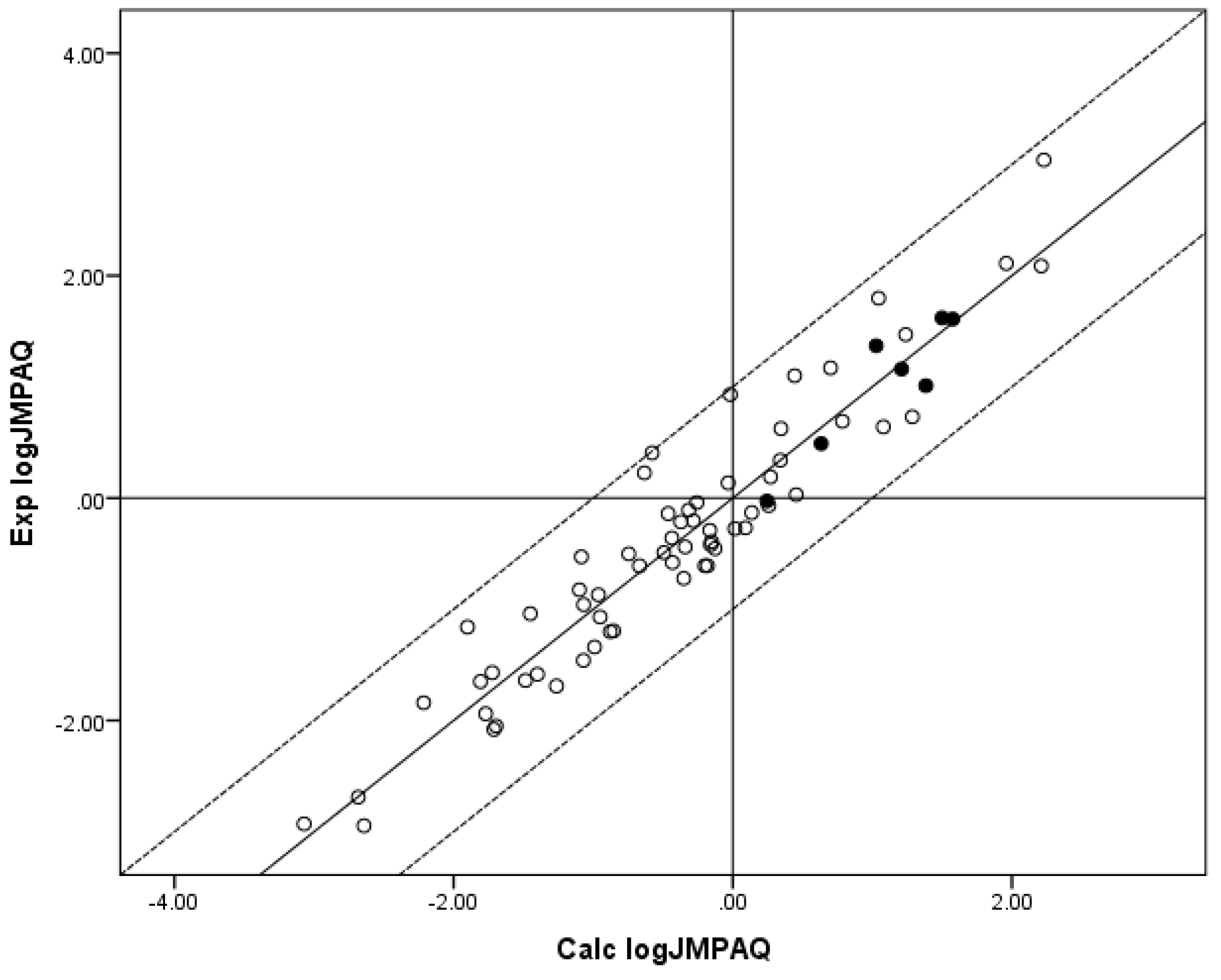
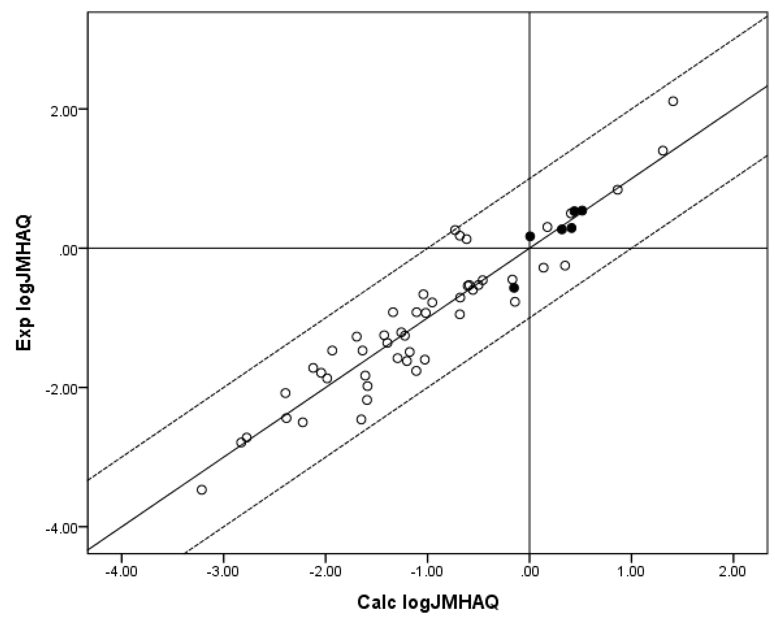
Figure 1,
Figure 2.
Figure 1 shows a plot of experimental (Exp.) log
JMPAQ versus log
JMPAQ calculated (Calc.) from the coefficients for the fit of the
n = 70 database to RS, and
Figure 2 shows a plot of Exp. log
JMHAQ versus log
JMHAQ Calc. from the coefficients for the fit of the
n = 55 database to RS.
Table 2.
The calculated (Calc.), predicted (Pred.), and experimental (Exp.) maximum flux values through silicone from water (log JMPAQ) and through human stratum corneum from water (log JMHAQ) for the n = 7 phenolic compounds.
Table 2.
The calculated (Calc.), predicted (Pred.), and experimental (Exp.) maximum flux values through silicone from water (log JMPAQ) and through human stratum corneum from water (log JMHAQ) for the n = 7 phenolic compounds.
| Cmpd. a | Exp. log JMPAQ b | Pred. n = 63 log JMPAQ b,c | Calc. n = 70 log JMPAQ b,d | Exp. log JMHAQ b | Pred. n = 48 log JMHAQ b,e | Calc. n = 55 log JMHAQ b,f |
|---|
| 1 | 1.01 | 1.41 | 1.40 | 0.29 | 0.46 | 0.41 |
| 2 | −0.027 | 0.28 | 0.26 | −0.95 | −0.66 | −0.68 |
| 3 | 1.37 | 1.05 | 1.04 | 0.17 | 0.087 | 0.0053 |
| 4 | 1.62 | 1.52 | 1.51 | 0.53 | 0.54 | 0.44 |
| 5 | 1.16 | 1.24 | 1.23 | 0.27 | 0.35 | 0.32 |
| 6 | 0.49 | 0.67 | 0.65 | −0.57 | −0.17 | −0.15 |
| 7 | 1.61 | 1.60 | 1.59 | 0.54 | 0.62 | 0.52 |
| Δlog
JMAQ g | | 0.200 | 0.195 | | 0.159 | 0.162 |
Figure 1.
The correlation of the calculated (Calc.) log JMPAQ from the fit of n = 70 to RS with the experimental (Exp.) log JMPAQ. The dashed lines represent the boundaries for residual log JMPAQ greater than 1.0, the solid line indicates points where the Calc. log JMPAQ is equivalent to the Exp. log JMPAQ. The filled circles indicate the n = 7 phenols. The Calc. log JMPAQ values were determined with Equation 5: log JMPAQ = −1.606 + 0.695 log SOCT + 0.305 log SAQ − 0.00490MW. r2 = 0.907, average absolute residual log JMPAQ = 0.300.
Figure 2.
The correlation of the calculated (Calc.) log JMHAQ from the fit of n = 55 to RS with the experimental (Exp.) log JMHAQ. The dashed lines represent the boundaries for residual Exp. log JMHAQ greater than 1.0, and the solid line indicates points where the Calc. log JMHAQ is equivalent to the Exp. log JMHAQ. The filled circles indicate the n = 7 phenols. The Calc. log JMHAQ values were determined with Equation 6: log JMHAQ = −3.005 + 0.654 log SOCT + 0.346 log SAQ − 0.00112 MW, r2 = 0.883, average absolute residual log JMHAQ = 0.282.
Plots of the individual independent variables, log
SOCT, log
SAQ and MW, against log
JMPAQ (
n = 70) and against log
JMHAQ (
n = 55) gave the following
r2 values: (a) log
JMPAQ versus log
SOCT,
r2 = 0.677;
versus log
SAQ,
r2 = 0.554;
versus MW,
r2 = 0.541; (b) log
JMHAQ versus log
SOCT,
r2 = 0.603;
versus log
SAQ,
r2 = 0.526;
versus MW,
r2 = 0.520. All regression equations had statistically significant (
p < 0.05) slope and intercept estimates. In each case, the best regression of the individual independent variables against flux values was by log
SOCT. It is worth noting that the
n = 7 phenol subset gives the following
r2 values and significance profiles when the individual independent variables log
SOCT and log
SAQ are plotted against log
JMPAQ and log
JMHAQ: (a) log
JMPAQ versus log
SOCT,
r2 = 0.180, without a statistically significant slope (
p = 0.34) or intercept (
p = 0.51);
versus log
SAQ,
r2 = 0.949, with a statistically significant slope (
p < 0.05), but without a statistically significant intercept (
p = 0.50); (b) log
JMHAQ versus log
SOCT,
r2 = 0.335, without a statistically significant slope (
p = 0.17) or intercept (
p = 0.18);
versus log
SAQ,
r2 = 0.933, with statistically significant (
p < 0.05) slope and intercept. The improved dependence of maximum flux from water on the aqueous solubility of highly water-soluble compounds is demonstrated here as a property of both silicone and human stratum corneum, and will be a topic of future investigations. When two individual independent variables, log
SOCT and MW, from the
n = 70 log
JMPAQ database were fitted to the KSC equation (Equation 3) the following
x,
y and
z coefficients to the parameters were obtained along with
r2 and Δlog
JMPAQ values:
x = −0.923,
y = 0.794,
z = 0.0089,
r2 = 0.797 and Δlog
JMPAQ = 0.431. All but the
y coefficient (
p = 0.069) were statistically significant (
p < 0.05):
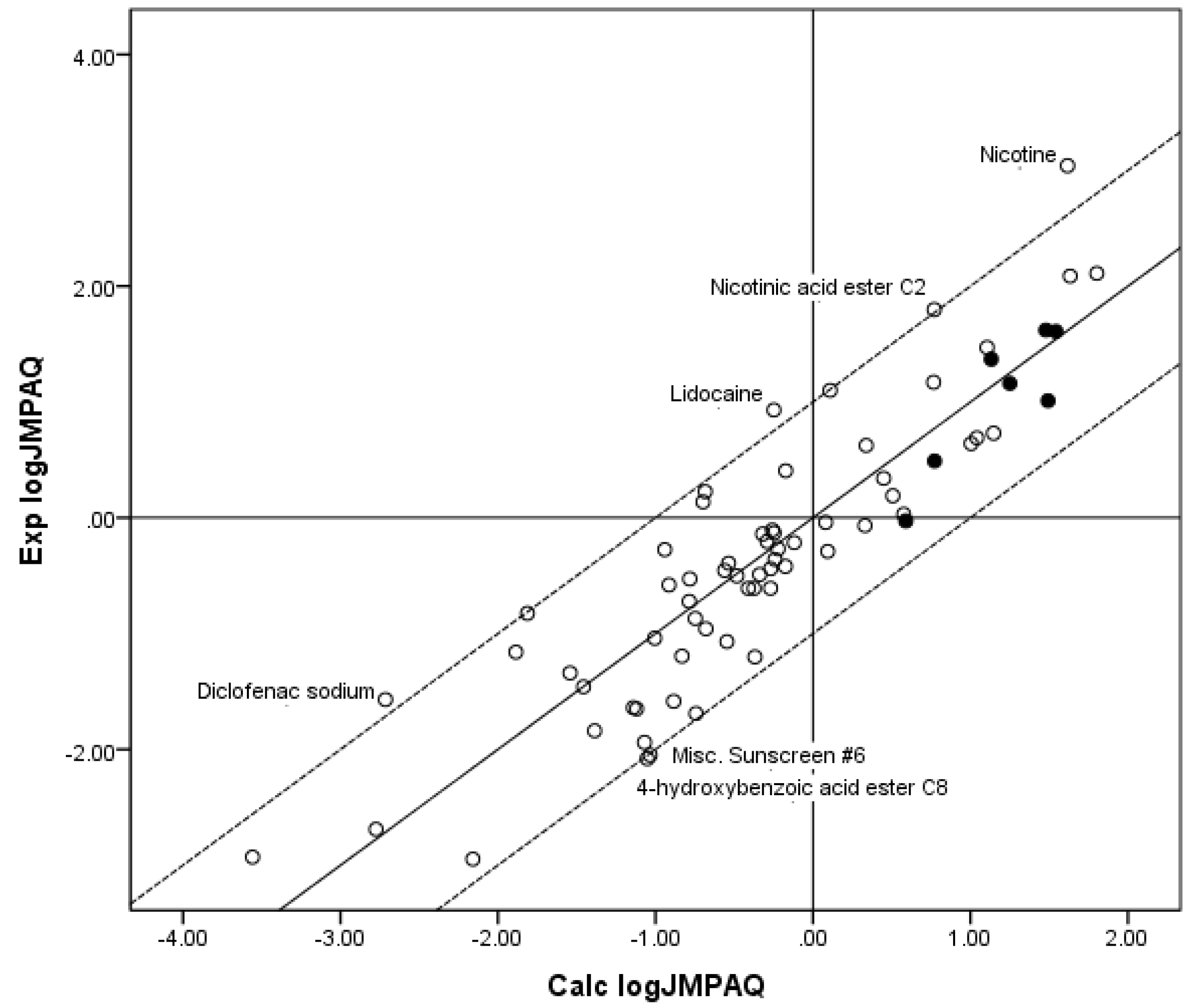
Figure 3 shows a plot of Exp. log
JMPAQ versus log
JMPAQ values calculated from the coefficients for the fit of the
n = 70 database to Equation 7. Although the
r2 was substantially improved by including MW with log
SOCT as independent variables in the regression against flux, the
r2 was poorer than the
r2 for the fit of all three independent variables to the Roberts–Sloan Equation (Equation 5). Similarly, when two individual independent variables, log
SOCT and MW, from the
n = 55 log
JMHAQ database were fit to the KSC equation (Equation 8) the following
x,
y and
z coefficients to the parameters were obtained along with
r2 and the Δlog
JMHAQ values:
x = −1.252,
y = 0.602,
z = 0.0080,
r2 = 0.723 and Δlog
JMHAQ = 0.441. The estimates for the coefficients were all statistically significant (
p < 0.05):
Figure 3.
The correlation of the calculated (Calc.) log JMPAQ from the fit of n = 70 to KSC with the experimental (Exp.) log JMPAQ. The dashed lines represent the boundaries for residual Exp. log JMPAQ greater than 1.0, the solid line indicates points where the Calc. log JMPAQ is equivalent to the Exp. log JMPAQ. The filled circles indicate the n = 7 phenols. The Calc. log JMPAQ values were determined with Equation 7: log JMPAQ = −0.923 + 0.794 log SOCT − 0.0089 MW, r2 = 0.797, average absolute residual log JMPAQ = 0.431.
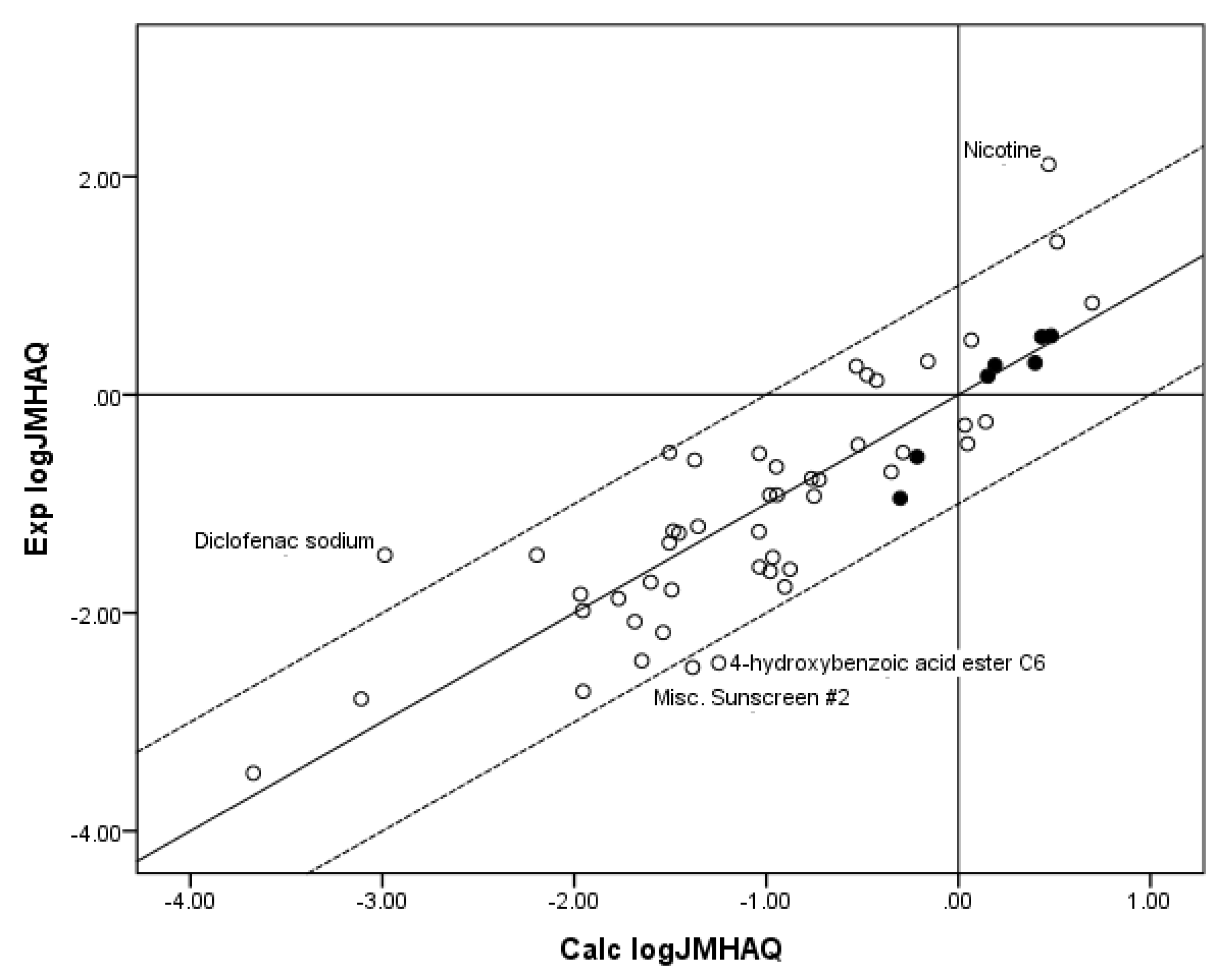
Figure 4 shows a plot of Exp. log
JMHAQ versus log
JMHAQ values calculated from the coefficients for the fit of the
n = 55 database to Equation 8. Again, although a substantial improvement in
r2 was obtained by including MW with log
SOCT as independent variables in the regression against flux, the
r2 was poorer than the
r2 for the fit of all three independent variables to the RS equation (Equation 6). The fit of both databases to the MACR equation (Equation 4), which is the remaining model used to predict maximum flux, is simply the regression of MW against log
JMPAQ or log
JMHAQ shown above to give a somewhat poorer fit than regression of the two individual independent variables, log
SOCT or log
SAQ, against log
JMPAQ or log
JMHAQ. Finally, it should be noted the popular Potts–Guy Equation [
14] was not included as a model because its output is permeability coefficient which is not clinically relevant.
Figure 4.
The correlation of the calculated (Calc.) log JMHAQ from the fit of n = 55 to KSC with the experimental (Exp.) log JMHAQ. The dashed lines represent the boundaries for residual Exp. log JMHAQ greater than 1.0, and the solid line indicates points where the Calc. log JMHAQ is equivalent to the Exp. log JMHAQ. The filled circles indicate the n = 7 phenols. The Calc. log JMHAQ values were determined with Equation 8: log JMHAQ = −1.252 + 0.602 log SOCT − 0.0080 MW, r2 = 0.723, average absolute residual log JMHAQ = 0.441.
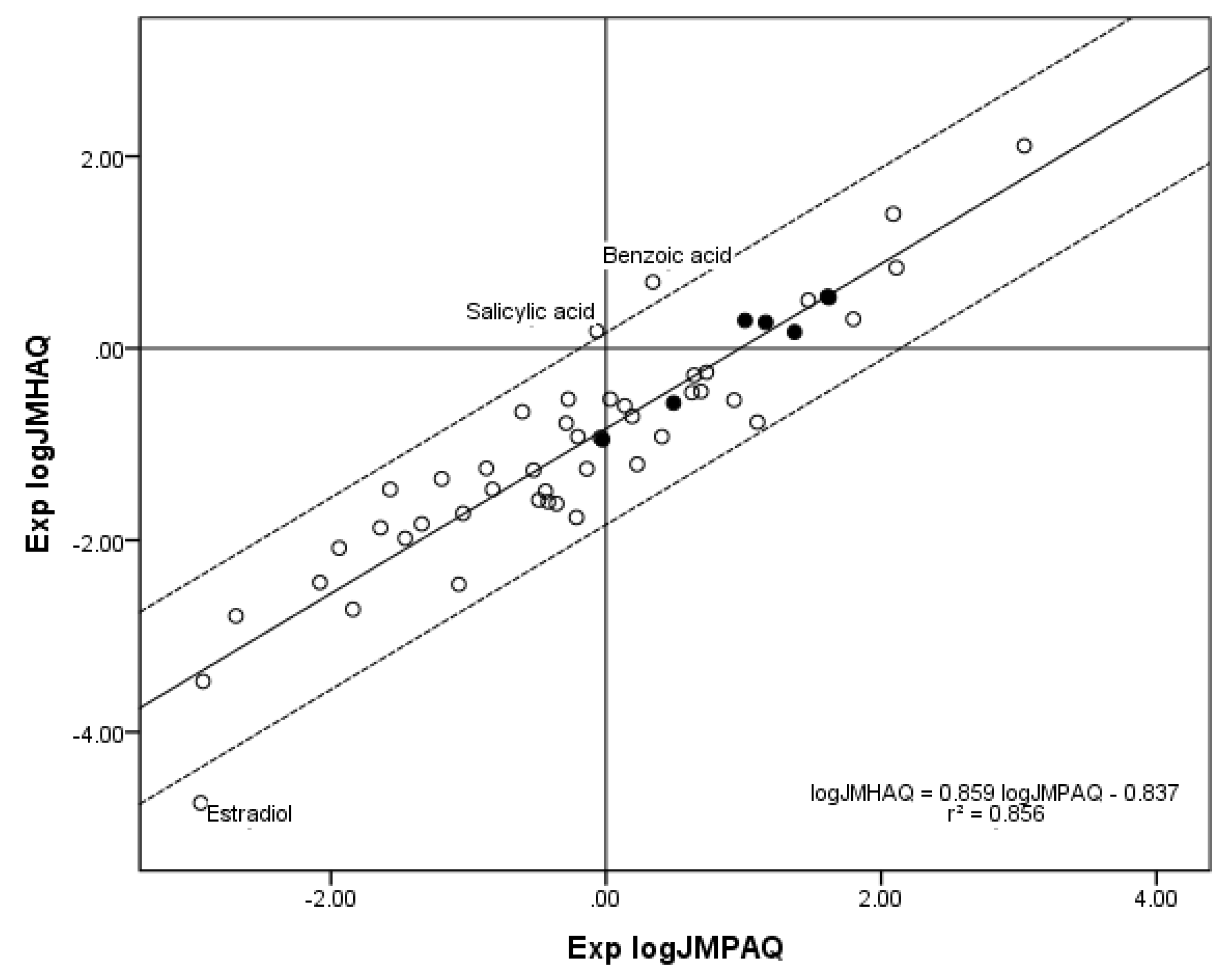
The new
n = 52 database of compounds contributing to both the
n = 70 log
JMPAQ database and the
n = 55 log
JMHAQ database also gives a higher correlation between Exp. log
JMPAQ and Exp. log
JMHAQ than the previous
n = 45 database. A linear regression yielded the expression Exp. log
JMHAQ = 0.859 Exp. log
JMPAQ − 0.837,
r2 = 0.856, which is an improvement over
r2 = 0.838 for the
n = 45 database.
Figure 5 shows the plot of Exp. log
JMPAQ versus Exp. log
JMHAQ for
n = 52.
Figure 5.
The correlation of the n = 52 log JMHAQ with log JMPAQ database. The dashed lines represent the boundaries for residual Exp. log JMHAQ greater than 1.0, and the solid line is the regression equation. The filled circles indicate the n = 7 phenols. The regression information is in the figure.


