Abstract
The need for innovative pathways for future zero-emission and sustainable power development has recently accelerated the uptake of variable renewable energy resources (VREs). However, integration of VREs such as photovoltaic and wind generators requires the right approaches to design and operational planning towards coping with the fluctuating outputs. This paper investigates the technical and economic prospects of scheduling flexible demand resources (FDRs) in optimal configuration planning of VRE-based microgrids. The proposed demand-side management (DSM) strategy considers short-term power generation forecast to efficiently schedule the FDRs ahead of time in order to minimize the gap between generation and load demand. The objective is to determine the optimal size of the battery energy storage, photovoltaic and wind systems at minimum total investment costs. Two simulation scenarios, without and with the consideration of DSM, were investigated. The random forest algorithm implemented on scikit-learn python environment is utilized for short-term power prediction, and mixed integer linear programming (MILP) on MATLAB® is used for optimum configuration optimization. From the simulation results obtained here, the application of FDR scheduling resulted in a significant cost saving of investment costs. Moreover, the proposed approach demonstrated the effectiveness of the FDR in minimizing the mismatch between the generation and load demand.
1. Introduction
The action plan for meeting the huge energy needs of developing countries includes the strategic design of small microgrids for areas that are not yet connected to the main grid due to technical and geographical limitations. Moreover, the global call for decarbonization of the current energy mix towards climate change mitigation has increased the call for a more sustainable energy supply system via renewable energy resources-based microgrid technologies [1]. A microgrid is a small power system consisting of a cluster of distributed energy generation resources, energy storage systems and aggregated loads that can operate in isolated mode or grid-connected mode for providing clean, reliable and affordable energy supply [2]. The technical aspect of the design of a microgrid’s energy supply systems entails three interrelated aspects which include; the capacity sizing, time-based energy supply unit scheduling and point-to-point energy transaction strategy [3]. Most research activities on microgrid design consider these aspects in a segregated approach; hence, there is a tendency to miss the link between the long-term investment requirements and the short-term operational requirements.
Achieving an optimum component sizing is highly essential for realising the long-term techno-economic goals of the microgrid system. However, the cost of short-term scheduling and energy transactions should be essentially factored in at the component sizing stage so as to achieve the best configuration in terms of overall cost benefits. More over, a system that considers only energy storage as a source of flexibility tends to be very expensive [4]; thus, there is a need to consider all possible resources that can contribute to overall power system flexibility enhancement [5,6]. The implementation of the DSM programs has the potential of acting as an ancillary system to meet the net-load by load profile reshaping. This will minimize the storage capacity requirement and subsequently reduce the total cost of investment on the microgrid. Hence, the transition to a sustainable, reliable and fully renewable energy-based microgrid development dictates the incorporation of demand-side management (DSM) [7] and other flexibility measures some of which involves smart energy management and energy resource forecasting [8].
As the penetration level of wind and solar energy resources increases, system resilience decreases due to the stochastic and intermittent changes in their output due to the weather conditions [9]. Thus, incorporating an effective forecasting technology can be a crucial supporting tool for wind and solar power coordination for DSM implementation into the smart microgrid network [10]. The cost benefits of incorporating the short-term forecasts of solar irradiance, wind speed and load demand in microgrid system operation planning are highlighted in [11,12]. A precise outlook of the expected generated power profile helped the system operator to achieve an efficient flexibility option for reliable operation planning by the utilities [13,14]. This involves intelligently scheduling the BESS operation to charge during peak generation periods and supplement the grid deficiencies during low power generation hours [15].
Furthermore, the advancement of smart grid technologies has brought remarkable improvement in efficiency, economics, and reliability of operation, especially in power systems with high renewable energy penetration [16]. The evolution of the smart grid requires the integration of the end-user devices, smart meters, advanced monitoring systems, communication infrastructure, substations, transmission lines, transformers, energy storage, protection systems, and so on, for efficient monitoring and control [17]. This transition requires the adoption of internet infrastructure as an enabling platform for monitoring, data acquisition, and system control of the power grid infrastructure by the utility, customer information dispensation, and the management of the flexible demand-side resources [18]. Hence, the utilization of an internet platform plays a significant role in the development and successful implementation of demand response and other demand-side management strategies.
The benefits of DSM in energy management planning has been well reported in the literature, especially from the economic perspective of customer electricity consumption [19,20]. Harnessing credible operational scheduling of the flexible demand resources capacity can yield sufficient operational flexibility from the demand side [21]. This benefit can ultimately translates to the economics of storage capacity sizing which can reduce the total investment cost and ensure a cheaper cost of electricity for the end user. With the implementation of appropriate DSM strategies with adequate energy resource forecasting, both the energy supplier and end-user can benefit when the customer alters their energy demand to benefit from the flexible pricing and incentives made available by the utilities.
This paper seeks to investigate the cost-effective configuration for achieving a totally renewable energy-based smart microgrid system. The renewable energy components considered are the wind and solar energy resources with battery energy storage system (BESS). To achieve the goal of this research, optimal component sizing is incorporated with and without DSM strategy and the cost of investment are compared. Moreover, the effectiveness of the incorporated energy management system is evaluated by considering the effects on the scheduling and system reliability. The capacity sizing optimization problem was formulated and solved as a mixed integer linear program implemented on the MILP solver of MATLAB® and the energy resource data modelling and forecasting is achieved using Scikit-learn tools in Python.
2. System Description and Modelling
Figure 1 shows the proposed schematic view of the microgrid. The proposed system considers two types of renewable energy generation sources; wind and solar energy and the BESS. The BESS stores excess power generated during the times of over-generation and supply energy back into the grid during power shortage. An integrated energy management system is also incorporated to provide the coordinated short-term operation management of the BESS and the FDR. The system is coordinated such that the use of shiftable loads tries to minimize the gap that exists between the electricity generation profile and consumption. The FDR are activated to consume surplus generation and are deactivated during periods of shortages.
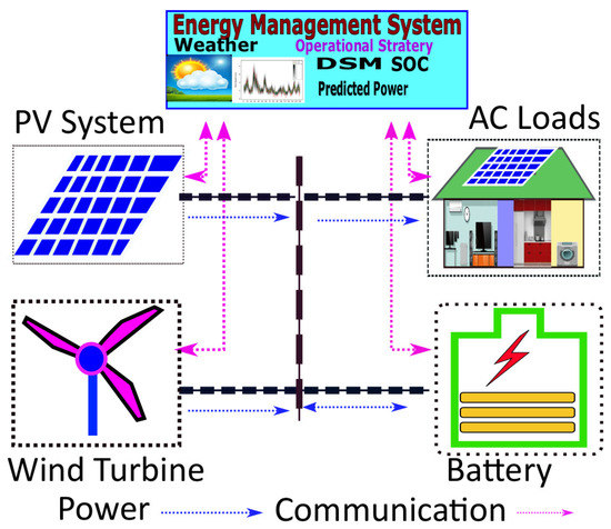
Figure 1.
Proposed schematic view of the microgrid.
2.1. Photo-Voltaic System Model (PV)
The instantaneous generated power output, of a PV system in kW with respect to the received solar irradiance, in W/m can be determined by using Equation (1):
where , expressed in percentage, is the PV module derating factor. The is the solar irradiance and is the rated capacity of the PV in kW under the standard test condition.
2.2. Wind Turbine Model
The instantaneous wind turbine generated power output depends on the speed of the wind at specified hub height. The power output of a WT can be described by using a piece-wise function described in Equation (2) as follows:
where is the rated power capacity of the WT, the , and is the cut-in, rated and cut-out wind speed of the wind turbine, respectively.
2.3. Battery Energy Storage System (BESS)
Whenever the total generation from the WT and PV exceeds the load demand, the BESS will switch into the charging mode. On the other hand, whenever the load demand exceeds the total generation, the BESS switches into the discharging state. The BESS state of charge at any given time t depends on the difference between the system load and the sum of the total renewable generation with the previous state of charge as the reference. The charging power or discharging power, as the case may be, is determined by the difference between the instantaneous load and generation. Hence, the current BESS state of charge at any given time, t (hour) is given by:
where and is the state of charge of the BESS for the current and previous time period in KWh respectively, is the hourly rate of self-discharge, and is the discharging and charging efficiency of the BESS, respectively. The minimum () and maximum () state of charge of the BESS are a function of the optimal capacity size as expressed:
where is the optimal capacity size of the BESS.
3. Demand-Side Management Strategy and Resource Forecasting
DSM programs are procedures that attempt to modify the energy demand of the power system in order to improve the overall system efficiencies. Appropriate implementation of DSM can provide the necessary operational flexibility by transferring the FDR from one period to another. Figure 2 illustrates the proposed planning framework for the system without and with DSM strategy consideration (Case 1 and 2, respectively). The objective of the planning framework is to minimize the total investment costs of the microgrid. The FDR planning is included as DSM strategy to implement effective scheduling scheme for the shiftable load demands. The FDR is activated to minimize the gap between generated power and load demand in the most cost-effective way based on sufficient system conditions. The scheduling of the FDR takes into consideration the difference between the forecasted total generation and the load demand by using the random forest prediction model. System constraints considered in the optimization comprise of both the capacity size limitation of the components (BESS, PV and WT) and the operational constraints of the BESS such as charging/discharging power, BESS state of charge, load demand and power supply balance, DSM and shiftable load capacity constraints.
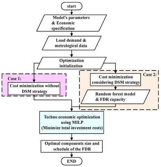
Figure 2.
Proposed smart microgrid planning framework.
3.1. Flexible Demand Resources Modeling
The scheduling of the FDR can be implemented in such a way that they are actuated to consume the surplus power during the period of in excess power generation and deactivated during periods of low power generation. The flexible demand resources (FDR) considered include, but not limited to, the heating and cooling loads, water pumping, washing machines, etc. The new load demands for any given time t after FDR scheduling is equal to the initial load demand plus or minus the shifted FDR capacity (), depending on the system load and generation balance dynamics per time.
The potential deferrable load capacity is taken to be 10% of the initial load demand as shown in the above Equation (7), and the total quantity of energy consumed before and after implementation of the FDR schedule is constrained to be equal.
where T is the total number of time steps in the scheduling horizon.
3.2. Wind and Solar Forecasting
The strong correlation between the received ground-level solar irradiance, and the generated output power of the PV system provides the flexibly to utilize the predictions of solar irradiance in estimating the output power of the PV in smart grid applications [22]. The same approach is also adopted in predicting the wind power output based on the wind speed forecasts. Therefore, solar irradiance and wind speed prediction are also equally crucial to the implementation of energy management in the smart grid [23]. The wind and solar power forecasting model implemented in this study considered the following input parameters; wind speed, solar irradiance, humidity, temperature, pressure and wind direction.
The model fitting or training of data-driven forecasting model is achieved by establishing underlying patterns among historical input variables [24]. Thus, its success relies heavily on appropriate input parameters selection, and the data pre-possessing. The candidate input data set for the model consists of a number of variables such as humidity, wind speed, pressure, solar irradiance, temperature, etc. A data-driven framework is based on the standard methodology of data science, and the main stages are as outlined; data pre-processing, model training, validation and final deployment. Data pre-processing might integrate all or some of these standard techniques: transformation, integration, normalization, cleaning etc. The subsequent process includes modeling, performance evaluation, and final deployment [25]. The schematic forecasting framework adopted in this study is shown in Figure 3.
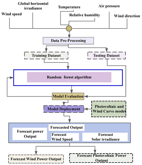
Figure 3.
Proposed schematic forecasting framework.
3.2.1. Random Forest Regression
Random Forest (RF) is a bagging ensembled-based machine learning algorithm combining several single models of classification and regression trees. The classical decision tree has a shortcoming of over-fitting the training data and variance tending to be high. Thus, the superior advantage of RF over other machine learning algorithms is adopted. The randomization methodology in the RF algorithm reduces the high model’s variance considerably [26]. The training of each decision tree is based on randomly selected attributes and randomly selected bootstrap samples from the training dataset [27,28].
3.2.2. Random Forest Algorithm
Algorithm 1 outlines the pseudo-code procedure of the random forest algorithm.
| Algorithm 1: Random forest pseudo-code |
| Prerequisite: Training data set M, n forest trees and P traits (Temperature, wind speed, solar Irradiance, etc.) |
| 1. Growing n forest trees. |
| 2. For |
| 3. Select a random sample from training set M. |
| with replacement. |
| 4. Grow a tree without pruning. |
| 5. Split-attribute: |
| Randomly select attribute n for splitting. |
| 6. Best split: |
| Evaluate the gain of split-attribute for samples. |
| 7. End For |
| 8. Provided a new data set y: |
| 9. Predict the new data by averaging the predictions of each individual n forest trees by averaging |
| 10. End: Terminate the algorithm |
For a training data set M, we extract a random sample with replacement, where i indexes the i-th bootstrap sample. Based on the decision-tree algorithm, we grow n trees for each bootstrap sample without pruning. For each tree, a restrained randomly selected data set attribute p is selected. p equals the number of split-attributes randomly selected out of all possible split attributes P: . The bounded selected attribute n is a subset of N and is always very small compared to P; . This superior property of the RF algorithm gives its fast speed trait and over-fitting elimination attribute. The outcome of the prediction is calculated by finding the averaging of the individual predictions of each tree.
3.2.3. Forecasting Error Metrics
The prediction results of the forecasting models are evaluated using the mean absolute error (MAE) [29], root means squire error (RMSE) and the metrics [30]. is a statistical performances metric that gives a measure of the closeness between the actual and predicted data. Its values range from 0 to 1 and validate the appropriateness of model selection. A value of 1 is an indication of a perfect fit model, while a value of 0 is a suggestion of the unsuitability of the selected model.
- MAE
- RMSE
- rwhere is the values of the predicted data, the and represent the actual and the mean of the input data respectively.
4. Sizing Optimization
The objective of the optimum component sizing is to minimize the Net Present Value (NPV) of the total investment costs (TIC). The investments cost entails the capital costs, operation and maintenance and the replacement costs of PV, WT and BESS. The optimization decision variables are optimum component sizing of PV, WT and the BESS.
4.1. Objective Function
4.2. Constraints
- Power balance constraint without FDR implementation:The total power generated should satisfy the energy demand at any given time.where is the load demand, and is the BESS discharging and charging power.
- Power balance constraint with the consideration of the FDR rescheduling program can be expressed as:
- BESS constraints: the energy stored in the BESS must be bounded within the minimum () and the maximum state of charge () limit.
- BESS maximum charging and discharging power is bounded by the maximum charging () and discharging power capacity ().
- Charging and discharging of the BESS cannot occur simultaneously.where and are the integer variables denoting the charging and discharging operation state of the BESS, respectively.
5. Simulation Parameters, Data Description and Case Study
The simulation system parameters for BESS, WT and PV are as summarized in Table 1. The hourly historical meteorological for the considered site was obtained from meteoblue [31] and NASA database for the year 2017 to 2019. The proposed approach in this study adopted an isolated microgrid in the Marsabit county of Kenya as a case study to evaluate and demonstrate the techno-economic gains of the proposed system flexibility management techniques. In order to demonstrate the efficiency of the proposed model, two simulation scenarios were considered as outlined below:

Table 1.
Simulation parameters for the proposed system.
- Case 1: Capacity optimization without DSM strategy.
- Case 2: Capacity optimization considering FDR scheduling as DSM strategy.
6. Simulation Results and Discussion
Based on the objective function and system constraints, as described in the formulations in Section 2, Section 3 and Section 4, mixed integer linear programming (MILP) is adopted as the optimization algorithm. The sizing optimization results for microgrid component size for two cases are presented in Table 2. Table 3 illustrate detailed investment costs per component and total system cost comparison for cases without and with DSM strategy consideration. For the two system configurations, the total energy consumed is considered to be equal. This implies that the application of the FDR scheduling scheme only impact the energy consumption pattern but doesn’t affect the total amount of the energy demanded by the end-users throughout the scheduling period.
Table 2.
Optimal components size and system configuration comparison without and with demand-side management (DSM) strategy consideration.
Table 3.
Investment costs per component and total system cost comparison for cases without and with DSM strategy consideration.
6.1. Optimum Configuration without DSM Strategy
As observed from Case 1 simulation results, the optimal system configuration obtained consists of 1196 kW, 2054 kW and 7150 kWh (with power converter capacity of 960 kW) component size of the PV, WT and the BESS, respectively. The minimum total investment costs for case 1 optimal system configuration is US $15,247,276.77 consisting of individual components costs for PV, WT and BESS as summarized in Table 2. Due to the variability of the renewable energy sources generation, the mismatch gap between the generation and load demand profiles tends to increase. With the incorporation of the BESS, an optimal configuration of PV-WT-BESS manages to meet the system load demand reliably. Figure 4 depicts the aggregated renewable power generation, BESS power and the load demand profiles without the consideration of the DSM strategy. As it can be observed, whenever the total generation surpasses the load demand, the surplus power is used to charge the BESS. In the event of deficit power generation, the BESS discharges to compensate the mismatch between the generation and load demand. Figure 5 and Figure 6 show the charging and discharging dynamics and the state of charge of the BESS, respectively, for case 1 optimal configuration. However, in this case, the optimal capacity of the BESS is relatively large, and thus, the total system costs are relatively expensive. Thus, the inclusion of the DSM strategy is essential.
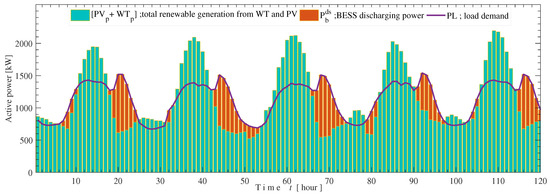
Figure 4.
Aggregated renewable power generation, battery energy storage system (BESS) power and the load demand profiles without the consideration of the DSM strategy (case 1).
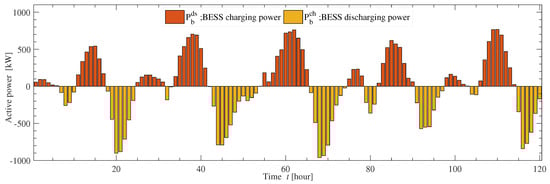
Figure 5.
Charging and discharging power and the dynamics of the BESS (Case 1).
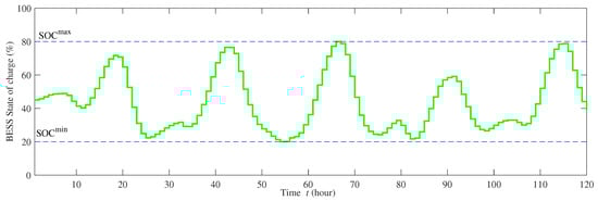
Figure 6.
BESS state of charge (case 1).
6.2. Optimum Configuration Considering DSM Strategy and Resource Forecasting
The time-ahead resource forecasts obtained using RF model are used to implement the FDR scheduling based on the anticipated mismatch between the generation and load demand. The forecasting results based on MAE, RMSE and performance metrics for wind speed, solar irradiances, wind and solar photovoltaic power are as summarized in Table 4.
Table 4.
Forecasting simulation results in terms of performance evaluation metrics.
As can be seen, the performance of the random forest forecasting algorithm depends on the selected size of the estimators. The number of estimators n represents the numbers of decision trees selected and grown at random with replacement during the training phase of the model. As it can be seen from the simulation results, the n values selected determines the accuracy of the RF forecasting model. As it can be observed, the best performances are obtained when the decision tree is set to 800 for the case of wind speed and wind power prediction. This is confirmed by the least error values indicated by the MAE and RMSE error metric values for wind speed and wind power forecast results. The appropriateness of the model and parameter estimation selection are validated by the highest value of the metric. Figure 7 shows a graphical comparison of the actual versus the predicted wind speed using the RF forecasting model. For the case of solar irradiance and PV power prediction, an estimator of n = 80 yields the best forecasting results. Figure 8 shows a graphical comparison of the actual versus the predicted solar irradiance using the RF forecasting model.
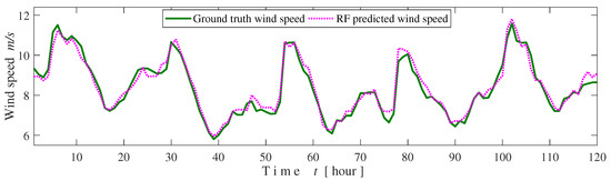
Figure 7.
A graphical comparison of the actual versus the forecasted wind speed with one-time step ahead rolling horizon using Random Forest (RF) forecasting model for (1/12/2018 to 5/12/2018).
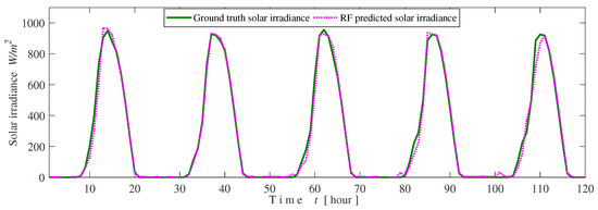
Figure 8.
A graphical comparison of the actual versus the forecasted solar irradiances with one-time step ahead rolling horizon using RF forecasting model for (1/12/2018 to 5/12/2018).
From the Case 2 simulation results, the minimum total investment cost is US $13,355,165.67 with an optimum size of the PV, WT and BESS equal to 1401 kW, 1866 kW and 5200 kWh (with power converter capacity of 820 kW), respectively. Figure 9 illustrates the aggregated generated power from renewable energy sources, BESS discharging power and the load demand profiles. Figure 10 and Figure 11 show the charging and discharging power and the SOC of the BESS for case 2, respectively.
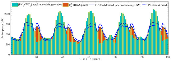
Figure 9.
Aggregated power generated, BESS discharging power and load demand profiles with DSM strategy inclusion (case 2).
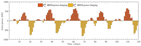
Figure 10.
BESS charging and discharging dynamics (case 2).
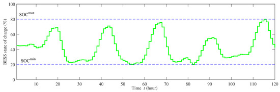
Figure 11.
BESS state of charge (case 2).
6.3. Techno-Economic Optimal System Configuration Comparison and Analysis
The application of the FDR scheduling program has demonstrated to have several techno-economic benefit to the optimum configuration planning of the microgrid system. As can be seen in Figure 9, the FDR rescheduling tends to shift the load demand from low generation periods to peak-generation periods. This DSM strategy attempts to minimize the gap between the generation profile and the load demand and thus decrease the system component capacities of the WT and BESS. The FDR shifting programs time shifts the flexible energy demands from deficit generation to surplus generation periods resulting in percentage cost proportion of the BESS to the total investment cost of 41.32% without DSM and 34.31% with DSM. The resultant system configuration with DSM resulted in a significant cost saving in the investment costs of about 12.41% with respect to the case 1 (without DSM). This investment cost saving is due to the ability of the DSM strategy to reduce the gap between generation and demand for most of the considered time instance. Its worth noting that the increase in PV capacity and decrease in WT optimal system configuration is due to costs per kW difference between the two technologies, PV system is relatively cheaper per kW compared to WT generation technology.
7. Conclusions
In this work, the incorporation of the DSM strategy for effective optimal configuration is presented as a transition pathway towards accelerating uptake and management of variable renewable energy sources for smart microgrid. The system model considered in this work consists of the PV, WT and BESS without and with FDR scheduling. Due to the variability of the renewable energy sources, the mismatch between the generation and load demand profiles tends to increase. Thus, FDR scheduling technique that attempts to minimize the instantaneous mismatch between the load demand and generation profiles is proposed towards reducing the overall system planning cost. The effectiveness of the proposed methodology was investigated and verified on a real Kenyan microgrid. The Kenyan microgrid was used as case study to demonstrate the proposed methodology and techniques due to the accessibility of the required data. However, the research parameter and simulation are obtained from general specification in existing literature. Hence, the procedure can be replicated anywhere in the world for any given smart energy hub or systems.
The objective is to determine the optimum size of the battery energy storage, photovoltaic and wind systems at minimum total investment costs. The results of short-term power generation forecasts are utilized to improve and effectively schedule the FDRs. Two simulation scenarios, without and with the consideration of DSM, were compared. From the simulation results obtained, the application of FDR scheduling resulted in a significant cost saving of about 12.41% of the investment costs. The FDR shifting programs time-shifted the flexible energy demands from deficit generation periods to surplus generation periods, thus; resulting in credible system component size reduction. Moreover, the proposed approach demonstrated the effectiveness of the FDR in minimizing the mismatch between the generation and load demand. Hence, this paper has shown the potential cost-benefit of FDRs scheduling DSM strategy consideration for effective optimal component sizing for current and future VRE-based smart microgrid developments.
Author Contributions
Conceptualization, M.K.K.; methodology, M.K.K., O.B.A. and M.E.L.; validation, T.S., T.A. and K.V.K.; formal analysis and investigation, M.K.K., O.B.A. and M.E.L.; writing–original draft preparation, M.K.K. and O.B.A.; writing–review and editing, M.K.K., O.B.A. and M.E.L.; supervision, project administration and funding acquisition, T.S.
Funding
This research received no external funding.
Acknowledgments
The authors wish to acknowledge the Japan international cooperation agency (JICA) for the support provided in the form of African business education (ABE) scholarship to the main author towards the success of this research work. The authors also wish to appreciate the effort of Hannington Gochi of REA, Kenya office for supplying the principal data needed for this project.
Conflicts of Interest
The authors declare no conflict of interest.
Abbreviations
The following abbreviations are used in this manuscript:
| REA | Rural Electrification Authority |
| ABE | African business education |
| JICA | Japan international cooperation agency |
References
- McCollum, D.L.; Zhou, W.; Bertram, C.; De Boer, H.S.; Bosetti, V.; Busch, S.; Després, J.; Drouet, L.; Emmerling, J.; Fay, M.; et al. Energy investment needs for fulfilling the Paris Agreement and achieving the Sustainable Development Goals. Nat. Energy 2018, 3, 589. [Google Scholar] [CrossRef]
- López-González, A.; Ferrer-Martí, L.; Domenech, B. Sustainable rural electrification planning in developing countries: A proposal for electrification of isolated communities of Venezuela. Energy Policy 2019, 129, 327–338. [Google Scholar] [CrossRef]
- Kiptoo, M.K.; Adewuyi, O.B.; Lotfy, M.E.; Senjyu, T.; Mandal, P.; Abdel-Akher, M. Multi-Objective Optimal Capacity Planning for 100% Renewable Energy-Based Microgrid Incorporating Cost of Demand-Side Flexibility Management. Appl. Sci. 2019, 9, 3855. [Google Scholar] [CrossRef]
- Adewuyi, O.B.; Shigenobu, R.; Ooya, K.; Senjyu, T.; Howlader, A.M. Static voltage stability improvement with battery energy storage considering optimal control of active and reactive power injection. Electr. Pow. Syst. Res. 2019, 172, 303–312. [Google Scholar] [CrossRef]
- Kristiansen, M.; Korpås, M.; Svendsen, H.G. A generic framework for power system flexibility analysis using cooperative game theory. Appl. Energy 2018, 212, 223–232. [Google Scholar] [CrossRef]
- Alizadeh, M.I.; Moghaddam, M.P.; Amjady, N.; Siano, P.; Sheikh-El-Eslami, M.K. Flexibility in future power systems with high renewable penetration: A review. Renew. Sustain. Energy Rev. 2016, 57, 1186–1193. [Google Scholar] [CrossRef]
- Amrollahi, M.H.; Bathaee, S.M.T. Techno-economic optimization of hybrid photovoltaic/wind generation together with energy storage system in a stand-alone micro-grid subjected to demand response. Appl. Energy 2017, 202, 66–77. [Google Scholar] [CrossRef]
- Majidi, M.; Nojavan, S. Optimal sizing of energy storage system in a renewable-based microgrid under flexible demand side management considering reliability and uncertainties. J. Oper. Autom. Power Eng. 2017, 5, 205–214. [Google Scholar]
- Pietzcker, R.C.; Ueckerdt, F.; Carrara, S.; De Boer, H.S.; Després, J.; Fujimori, S.; Johnson, N.; Kitous, A.; Scholz, Y.; Sullivan, P.; et al. System integration of wind and solar power in integrated assessment models: A cross-model evaluation of new approaches. Energy Econ. 2017, 64, 583–599. [Google Scholar] [CrossRef]
- Sheth, A.; Gautam, P.; Siridevi, N.C. Intelligent Generation Scheduler for a Smart Micro Grid. In Proceedings of the 2018 2nd International Conference on Power, Energy and Environment: Towards Smart Technology (ICEPE), Shillong, India, 1–2 June 2018. [Google Scholar]
- Esfetanaj, N.N.; Nojavan, S. The Use of Hybrid Neural Networks, Wavelet Transform and Heuristic Algorithm of WIPSO in Smart Grids to Improve Short-Term Prediction of Load, Solar Power, and Wind Energy. In Operation of Distributed Energy Resources in Smart Distribution Networks; Elsevier: Amsterdam, The Netherlands, 2018; pp. 75–100. [Google Scholar]
- Notton, G.; Nivet, M.L.; Voyant, C.; Paoli, C.; Darras, C.; Motte, F.; Fouilloy, A. Intermittent and stochastic character of renewable energy sources: Consequences, cost of intermittence and benefit of forecasting. Renew. Sustain. Energy Rev. 2018, 87, 96–105. [Google Scholar] [CrossRef]
- Gürtler, M.; Paulsen, T. The effect of wind and solar power forecasts on day-ahead and intraday electricity prices in Germany. Energy Econ. 2018, 75, 150–162. [Google Scholar] [CrossRef]
- Martinez-Anido, C.B.; Botor, B.; Florita, A.R.; Draxl, C.; Lu, S.; Hamann, H.F.; Hodge, B.M. The value of day-ahead solar power forecasting improvement. Sol. Energy 2016, 129, 192–203. [Google Scholar] [CrossRef]
- Hodge, B.M.; Martinez-Anido, C.B.; Wang, Q.; Chartan, E.; Florita, A.; Kiviluoma, J. The combined value of wind and solar power forecasting improvements and electricity storage. Appl. Energy 2018, 214, 1–15. [Google Scholar] [CrossRef]
- Wang, K.; Wang, Y.; Hu, X.; Sun, Y.; Deng, D.J.; Vinel, A.; Zhang, Y. Wireless big data computing in smart grid. IEEE Wirel. Commun. 2017, 24, 58–64. [Google Scholar] [CrossRef]
- Rana, M. Architecture of the Internet of energy network: An application to smart grid communications. IEEE Access 2017, 5, 4704–4710. [Google Scholar] [CrossRef]
- Morello, R.; De Capua, C.; Fulco, G.; Mukhopadhyay, S.C. A smart power meter to monitor energy flow in smart grids: The role of advanced sensing and IoT in the electric grid of the future. IEEE Sens. J. 2017, 17, 7828–7837. [Google Scholar] [CrossRef]
- Wu, Z.; Tazvinga, H.; Xia, X. Demand side management of photovoltaic-battery hybrid system. Appl. Energy 2015, 148, 294–304. [Google Scholar] [CrossRef]
- Hussain, M.; Gao, Y. A review of demand response in an efficient smart grid environment. Electr. J. 2018, 31, 55–63. [Google Scholar] [CrossRef]
- Ogunjuyigbe, A.; Ayodele, T.; Akinola, O. Optimal allocation and sizing of PV/Wind/Split-diesel/Battery hybrid energy system for minimizing life cycle cost, carbon emission and dump energy of remote residential building. Appl. Energy 2016, 171, 153–171. [Google Scholar] [CrossRef]
- Alhussein, M.; Haider, S.I.; Aurangzeb, K. Microgrid-Level Energy Management Approach Based on Short-Term Forecasting of Wind Speed and Solar Irradiance. Energies 2019, 12, 1487. [Google Scholar] [CrossRef]
- Wan, C.; Zhao, J.; Song, Y.; Xu, Z.; Lin, J.; Hu, Z. Photovoltaic and solar power forecasting for smart grid energy management. CSEE J. Power Energy Syst. 2015, 1, 38–46. [Google Scholar] [CrossRef]
- Persson, C.; Bacher, P.; Shiga, T.; Madsen, H. Multi-site solar power forecasting using gradient boosted regression trees. Sol. Energy 2017, 150, 423–436. [Google Scholar] [CrossRef]
- Amasyali, K.; El-Gohary, N.M. A review of data-driven building energy consumption prediction studies. Renew. Sustain. Energy Rev. 2018, 81, 1192–1205. [Google Scholar] [CrossRef]
- Painsky, A.; Rosset, S. Lossless Compression of Random Forests. J. Comput. Sci. Technol. 2019, 34, 494–506. [Google Scholar] [CrossRef]
- Huertas Tato, J.; Centeno Brito, M. Using smart persistence and random forests to predict photovoltaic energy production. Energies 2019, 12, 100. [Google Scholar] [CrossRef]
- Barbosa de Alencar, D.; de Mattos Affonso, C.; Limão de Oliveira, R.; Moya Rodríguez, J.; Leite, J.; Reston Filho, J. Different models for forecasting wind power generation: Case study. Energies 2017, 10, 1976. [Google Scholar] [CrossRef]
- Kim, S.G.; Jung, J.Y.; Sim, M.K. A Two-Step Approach to Solar Power Generation Prediction Based on Weather Data Using Machine Learning. Sustainability 2019, 11, 1501. [Google Scholar] [CrossRef]
- Huang, C.J.; Kuo, P.H. A short-term wind speed forecasting model by using artificial neural networks with stochastic optimization for renewable energy systems. Energies 2018, 11, 2777. [Google Scholar] [CrossRef]
- Weather History Download. Available online: https://www.meteoblue.com (accessed on 13 July 2019).


© 2019 by the authors. Licensee MDPI, Basel, Switzerland. This article is an open access article distributed under the terms and conditions of the Creative Commons Attribution (CC BY) license (http://creativecommons.org/licenses/by/4.0/).