1. Introduction
The collection of spatio-temporal data is commonplace today—prime examples are user-generated data from mobile devices or social platforms, streams of sensor data from static or moving sensors, satellite or remote sensing data. To make sense of this vast volume of heterogeneous data, a variety of aggregation and fusion steps have to be applied to achieve semantic data enrichment for subsequent use in value-added services. However, enabling these enrichment steps generally relies on stable and highly scalable data handling and storage infrastructures. However, with ever increasing volumes of spatio-temporal data relational database technology (even with special object-relational extensions for spatio-temporal data) is stretched to its limits and currently new paradigms commonly referred to as ’Not Only SQL’ (NoSQL) databases are tried out as more scalable replacements, see, for example, Ref. [
1].
Given the significant amount of data logged daily with geotags and timestamps (see e.g., Ref. [
2]) and considering the distributed and global/local nature of such spatio-temporal data, simple
graph structures as basic representations become quite natural: traffic information in a road network, the spreading of epidemics over adjacent geographic regions, or time series data for chains of events. In a nutshell, graphs are composed of vertices (nodes) and edges (relations) joining two vertices together. Graph databases form an integral part of a group of NoSQL database technologies offering flexible and scalable solutions for many enterprise level problems. In a graph database, a vertex could be a user, business, vehicle, or city and edges could represent adjacency, roads, or location affiliations. Due to the relational nature of graphs, they are already used to model a wide variety of real-world phenomena such as physical, biological, and social information systems [
3].
However, although many categories of data are interpreted as graph structures today, traditional relational databases still lack the architecture and high-level query languages to effectively model and manipulate such structures. Graph databases are designed to represent data as attributes on vertices and edges. They are often schema-less (i.e., there is no fixed data structure) and their attributes are described as simple key-value pairs. Thus, a major strength of graph databases is that they excel in complex join-style queries where relational databases are notoriously inefficient for large tables [
4]. In contrast, graph databases tend to perform poorly when moving from local subgraphs to full graph aggregate queries, where relational database technology plays out its strength.
This paper investigates the suitability of which database technology is best suited to handle large-scale, spatio-temporal data in typical data manipulation tasks under real world settings. In particular, the investigation will cover the query speed, expressiveness of the available query languages, and computational demand on the open source graph database JanusGraph, the open source object-relational database system PostgreSQL, and the enterprise level graph analytics platform TigerGraph.
To allow for a fair and authoritative evaluation, on the one hand we use a real world data set for benchmarking. On the other hand, we use a simulation dataset offering more control to test the limits of the database technology used. For the real world data, Yelp is an internationally operating business directory service and review forum. The ‘Yelp dataset’ is a current subset of Yelp’s businesses, reviews, and user data comprising spatio-temporal data for 10 metropolitan areas across two countries with about 200,000 businesses and 6.6 million reviews. It is offered for academic use in the yearly Yelp challenge [
5], for a variety of data analysis and discovery tasks.
In contrast, the ambulance response simulation dataset [
6] from Umeå University, Sweden, offers more control over the scenario—given a number of hospital resources such as dispatch centres and ambulances, it simulates how emergency calls would be responded to by ambulances. The dataset records spatio-temporal properties such as the time intervals within the response life cycle and the origin and destination of the resource during the response. Other technical properties regarding the emergency itself are also recorded. In summary, we evaluated on two datasets with different representations of spatio-temporal properties, complexities from additional attributes, and total size.
Our contributions can be summarized as follows:
modelling and importing two characteristic datasets into three state of the art databases,
rigorously benchmarking them using various analyses that fairly represent the type of querying and data manipulation the dataset would typically undergo, and
comparing the suitability of JanusGraph vs. TigerGraph by investigating their specific graph query language implementations.
2. Problem Setting & Research Questions
This paper tackles the problem of modelling, visualizing, and querying large-scale spatio-temporal data using traditional relational database versus graph databases approaches. We investigate query performance, storage and computational cost, as well as ease and efficiency of simulation of real-world applications. In particular:
How to store spatio-temporal data efficiently? Coordinates are comprised of latitude and longitude and time adds a third dimension. The accessing times of secondary storage is an issue when housing large volumes of data. The use of R-Trees and a geo-graph (a grid-based geospatial system where vertices are grids and edges connect other vertices to these grid vertices to indicate their physical location) are two techniques investigated for efficiently indexing multidimensional data.
How to query a graph topology effectively? Basic graph pattern matching is popular when extracting data from graph databases, but there are a range of graph query languages (such as Gremlin, Cypher, and GSQL) implementing more complex graph patterns too. The conciseness of querying graphs versus traditional SQL is briefly addressed in the conclusion (
Section 7).
Can the respective database components be easily integrated into applications? Due to the rise of popularity in web-based applications, the ease of incorporating three typical databases into applications will be investigated with a Flask [
7] back-end and Angular [
8] driven front-end. This will show how appropriate it is in real-world applications and production settings to use graph database technologies and any challenges encountered during implementation versus using a classical SQL database back-end.
PostgreSQL was chosen as our control database due to its industry-proven suitability for spatio-temporal data when coupled with PostGIS. We chose two graph databases with differing underlying architectures, namely Java and C++, and compared how they performed against our control database and with respect to each other. Despite this choice in databases, there are other notable mentions such as GeoMesa [
9] and TerraLib [
10] as proven suitable alternatives for the analysis of spatio-temporal data.
3. Related Work
Whereas
relational databases generally store data in fixed-structure tuples within relations represented as tables and with foreign keys as interlinking elements, graph-based storage schemes allow for some more flexibility by focusing on simple data items (such as entities or attribute values) and their individual relationships. Especially highly tuned implementations of column stores [
11] or key-value stores [
12], often referred to as
NoSQL databases, gained traction for high volume data processing tasks in distributed and often quite heterogeneous environments [
4]. NoSQL is generally designed to run on multiple nodes, scale horizontally, and allow for massively parallel processing, see for example, Ref. [
13], yet comes at the price of being schema-less. Finally,
graph databases apply a richer graph structure to store and manipulate data as a good compromise between inflexible fixed-structure storage and schema-less storage tuned for efficiency. Data can be stored as key-pair attributes on both the vertices or edges of the database. In a nutshell, graph databases are strong at finding patterns and revealing information about the relationship between vertices rather than running aggregate queries on the data itself. Graph databases typically make data persistent using a ready-made storage back end. This can be a NoSQL database, as in JanusGraph, or a relational database, as in Facebook Tao’s case [
14].
In the following we will briefly summarize current contributions to particular data storage designs of all three basic storage models for spatio-temporal data mining, analysis, and visualization. Spatio-temporal data is constantly being generated by GPS-equipped devices everyday [
2,
15] and has important applications in epidemiologic [
16], marine, disaster relief, and social data investigation [
17]. In terms of structure, spatio-temporal data often shows strong ties between vertices representing physical locations and their association with other entities in the database. Thus, relational databases might come close to what is required in this setting due to their ability to manipulate data based on strongly structured table relations.
Yet, Moniruzzaman & Hossain [
18] elaborate on the specific shortcomings of relational database technologies in terms of performance when distributed over geographically diverse data centers due to their strong emphasis on consistency while maintaining ACID -compliance. Due to the current trend of hosting services in the cloud and the high velocity of incoming data and requests, a horizontally scalable, distributed system might thus, be better suited to address these issues, which would suggest a NoSQL solution. Still, a current benchmark by Makris, et al. [
1] compares how MongoDB (with GeoJSON) and PostgreSQL (with PostGIS) perform on large volumes of spatial data and shows that PostgreSQL actually outperforms its NoSQL rival.
On the other hand, the special kinds of spatio-temporal relations deeply embedded in spatial data are bound to determine specific ways how typical queries are written. Chen [
3] claims that practical queries in graph databases are usually designed to reveal hidden trends among the relationships in the data (especially when visualized) rather than within the data itself adding additional value in this implementation. Moreover, time adds an ordinal relation among all entries in the data that hold this property. Thus, in terms of efficiency graph databases may be a good compromise to answer complex questions on complex data. Such complex questions are typically ’multi join’-style queries, which are generally expensive, but whose evaluation might strongly benefit from exploiting any given schema information. Thus, a useful benchmark has to answer which technology would perform best not only in terms of performance, but also in terms of expressive querying, modeling, and visualizing of spatio-temporal data.
4. Design and Architecture
In this section we describe the design of the software, architecture, and technologies used to create the benchmark web-application. The analysis being performed by the web-application, how it performs each analysis, and how the backend queries each database is discussed.
4.1. Database Technologies
This section covers the underlying technologies used to implement the databases being benchmarked. This is important to note in terms of how portable each technology is, how difficult the configuration is before each database can be used for a given project, or limitations on performance or hardware requirements due to software requirements. While each database technology has varying capabilities, in terms of being supported for a given operating system, they each provide support for being deployed in a containerized environment.
PostgreSQL is a classical object-relational database queried via SQL queries. It is built to be extensible with a variety of existing extensions for additional features such as spatial indexing and thus caters for different kinds of data. PostgreSQL is quite a mature product often used in industrial applications and has a large amount of support from the open-source community. PostgreSQL version 11 and for the spatial extension PostGIS version 2.5 are used in this investigation.
JanusGraph [
19] is a highly scalable graph database ready to be clustered between multiple machines. JanusGraph is largely based on the Apache tech-stack making use of the property graph model from Apache TinkerPop. The native language through which JanusGraph is queried is Gremlin, but it can also be extended for Cypher queries. JanusGraph can store graph data via three backends: Apache Cassandra, Apache HBase, and Apache Berkeley. The configuration of JanusGraph used in this paper is with Apache Cassandra as the storage backend and ElasticSearch as the search engine for spatial and temporal query support. JanusGraph version 0.4 is used in this investigation.
TigerGraph is an enterprise level graph analytics platform developed with insights from projects such as Apache TinkerPop and Neo4j and provides advanced features like native parallel graph processing and fast offline batch loading, see Refs. [
20,
21]. Unlike JanusGraph, TigerGraph was developed from scratch in order to effectively create the next generation of graph database technology. Some of the use cases explicitly mentioned by TigerGraph (
https://www.tigergraph.com/solutions/) are in geospatial and time series analysis. TigerGraph is queried using the GSQL querying language. GraphStudio is a web interface which is packaged along with TigerGraph which provides an interface to write, install and visualize queries, design and export one’s graph schema, and monitor database performance. TigerGraph version 2.5 is used in this investigation.
4.2. Web-Application for Benchmark Simulation
For the benchmarking we designed a web-application on spatio-temporal data called Providentia. It is used to queue analysis tasks in a pipeline on which each benchmark is to be run, server performance measured, and accumulated results displayed. The architecture and how each technology communicates is illustrated in
Figure 1. The databases are containerized using Docker (
https://www.docker.com/).
Our first motivation towards using a commonplace Python backend is to make analysis setting realistic for the benchmark. Another advantage is that a simple REST API can be easily and quickly designed and deployed using the Flask framework. Angular was subjectively chosen as the front end framework as it allows for fast front end web development. All benchmarking results are stored in a separate database within PostgreSQL. Unfortunately, JanusGraph has some Java specific features that add limitations when making use of embedded Gremlin in Python. The limitations are, when trying to make use of mixed indexing search predicates such as spatial queries, that one may only do this via Java or a superset language thereof. The workaround for this was to make use of the Gremlin Translator which takes a Gremlin query as a string and interprets it on the server side.
The front end of Providentia allows a user to query each database, test the sentiment classifier, add benchmarking jobs and to review the performance and results of each analysis. Each job is run serially to avoid too much interference and competition between each database for resources. At intervals the CPU performance and memory consumption is measured and stored in PostgreSQL. The server performance and results of an analysis can be viewed together to validate that the outputs are the same and how each database utilizes the server’s resources.
4.3. Data Analysis Tasks in the Benchmark
Using each of the databases, a number of data analysis jobs are performed on the data. This section describes what each analysis aims to do and how they align to a typical real world use case. Each of these jobs have some kind of spatio-temporal aspect to test the accessibility of the data to demonstrate how well each database handles the data. These analysis are run over different percentages of the data loaded in each database and the performance is then measured and discussed in
Section 6. This section goes into more detail about the types of queries written and how well each language expresses each query.
4.3.1. Sentiment Analysis for Analysis Use Cases
Sentiment analysis is a class of natural language processing where subjective information is extracted from some given text [
22]. As a ground truth for all our benchmarking use cases, a simple binary sentiment classifier is used to classify the text of reviews as representing either a positive or negative sentiment. All natural language processing is done using the Natural Language Toolkit (NLTK—
https://www.nltk.org/) for Python. Then NLTK’s Naïve Bayes classifier was used to train and classify sentiment. Naïve Bayes is a probabilistic machine learning model which has proven very effective in text classification. A limitation of this model, on a binary classification problem, includes only being able to perform linear separability. This should not be an issue regarding the use of adjectives as feature vectors, since the most informative adjectives seem to be particular to a specific sentiment, for example, words such as ’horrible’, ’disgusting’, ’perfect’, or ’wonderful’ [
23].
4.3.2. Analysis Use Cases and Respective Kernels
Each of the following kernels represents some kind of user story for data analysis, in particular featuring some spatio-temporal constraint which will be applied on the respective queries. Each of these kernels will be benchmarked 30 times each, thus the mean and standard deviation can be considered when comparing response times. For each kernel, the respective database queries are available in
Appendix A.
Yelp: Kate’s Restaurant Recommendation
This analysis focuses on Kate, a user close to the beginning of the dataset having a number of reviews for restaurants in the Las Vegas area. A subset of reviews which hold a strictly greater than 3 star rating by Kate are selected, sorted by date descending, and limited by 10 reviews per user in order to take only the most relevant ones. These businesses are then selected, filtered by category ’Restaurants’. The users who have a star rating equal to or greater than Kate’s ratings for the same businesses are selected as the recommending users. Now assume that Kate has relocated to a new area. All businesses which have been rated strictly larger than 3 stars by the recommending users are then selected as restaurants to recommend to Kate in the new area. The text in these reviews are checked for sentiment and the percentage of positive sentiments is displayed alongside the average star rating for each recommended restaurant. This sentiment vs. average star rating is used as a metric to analyse in terms of asking the question: How reliable is the star rating versus the actual sentiment found in the text? The purpose of the first part of this kernel is to test the performance of a 1-hop graph traversal pattern. This hop is demonstrated in category filtering and finding users with mutual sentiment for a given review. This type of situation is faced by many recommendation technologies. The additional challenge is the relocation of Kate and seeing how responsive the database is to the spatial and temporal aspect, which form the second part of this kernel. The accumulated list of users is split into a separate query for each user to test the ability of each database technology to perform concurrent reads on subsets of data.
Yelp: Review Trends in Phoenix 2018
This analysis (summarized in
Figure A7,
Figure A8 and
Figure A9 in
Appendix C) goes deeper into observing the trend of various characteristics of reviews versus their star ratings. This is a common analysis performed on the Yelp dataset [
24], but the version in this investigation selects a subset of reviews only within the 2018 year in the Phoenix area. The spatio-temporal boundaries placed on this subset may reveal hidden trends to be considered in future work. Reviews are extracted first by location then by date. The reviews are then separated by star rating. For each star rating, the characteristics of ’funny’, ’useful’, and ’cool’ are accumulated and the text is classified as either positive or negative. For each star rating these are normalized and placed next to one another to see the characteristic of a review from each star group.
Yelp: Ranking Las Vegas by Friends’ Sentiment
The purpose of this analysis is the ability to aggregate relations from depth 1–2 of a graph pattern while maintaining spatio-temporal constraints. The user story of this kernel is that a user in the dataset would like to travel to Las Vegas over the November–December period. Instead of this user reading reviews from each of the hundreds of direct friends to the thousands of mutual friends, the sentiment from the reviews written by all direct and mutual friends during the November–December period (irrespective of year) in the Las Vegas area will be analysed. These reviews will be filtered by the spatial constraint of whether they are connected to businesses within 30 km of the Las Vegas center. The remaining reviews will have their text data extracted and returned for analysis. Using the sentiment classifier, a percentage positive sentiment will be generated and this will be the result of the data analysis.
Medical: Priority 1 Mean Response Times
This analysis (summarized in
Table A2 in
Appendix C) looks at the mean of two intervals within the response life cycle namely; travel time to the hospital and the time taken for the ambulance to start driving to the patient. This will filter out all responses which do not take the patient to the hospital and responses without a priority of 1 (highest). One hospital is isolated during this query. This query is useful in post-simulation analysis when optimizing response times with respect to a specific hospital. This can be extended to be grouped by hospitals if labels are associated with the coordinates.
Medical: Second Resource to Transfer Patients
During a response, sometimes multiple resources need to be sent depending on varying evaluation criteria made either by the call receiver or first resource upon arrival at the scene. This analysis (summarized in
Table A3 in the
Appendix C) considers how many resources, grouped by priority, were sent as the second resource to the same destination hospital from the kernel used above. This analysis can be used to investigate each priority’s resource usage and if their priority was perhaps misclassified. It can be further extended to look at third and fourth resources in order to be more thorough with the analysis.
Medical: Long Response Count
This analysis (summarized in
Table A4 in
Appendix C) is purely temporal and combines the time intervals from when the ambulance leaves up until the point where the patient is delivered to a hospital. The number of responses are returned for all responses which take longer than 15 min. This analysis could be useful when considering introducing a new hospital into a given area to improve response times.
5. Implementation
The following section describes how the systems were set up and data was preprocessed and describes the indexes used in each technology. The diagrams illustrating each of the databases’ schemas can be found under
Appendix B.
5.1. Benchmark Setup
5.1.1. Hardware Platform
All experiments were run on two setups detailed in
Table 1. Using these setups made it possible to consider how the technologies utilize multiple cores and perform with different storage limitations.
5.1.2. Data Sets
The first data set used is from the Yelp Dataset Challenge [
5]. Due to the large volume of the data set totaling 8.69 gigabytes in uncompressed format and hardware limitations, only subsets of the data are used to observe how well each database scales. These subsets were queried incrementally based on the percentage of users and businesses, that is, 10% would mean 10% of
business.json and 10% of
user.json. All of the reviews between the remaining users and businesses from
review.json are applied afterwards. The data set is stored as non-valid JSON and first had to be preprocessed and converted into valid JSON. During preprocessing many attributes not used in the analysis or benchmarking were removed to save on import time and storage costs. Only businesses, users, and reviews were used from the dataset. This resulted in a
reduction in uncompressed storage size, significant reduction in complexity and improvement in consistency among attributes. Aggregated attributes such as
average_stars and
review_count are removed, since such aggregates are invalid when working only with subsets of the data. The result of this preprocessing and feature selection can be seen in
Table 2.
The second dataset used is the medical response dataset (
Table 3) bcontaining 7568 records. This dataset represents one simulated year of ambulance responses. The spatial properties are originally based on a Cartesian coordinate system. Unfortunately, JanusGraph’s geo-predicates only support a geographic coordinate system. To support this limitation, a ’Flat Earth’ projection is used to convert the Cartesian points into latitude and longitude during the data normalization process. The
transfer attribute indicates whether the response resulted in on-site treatment or transport to a hospital which indicates if the
travel_time_station or
travel_time_hospital attributes are non-zero respectively.
5.2. Schema Design
The following section describes the different indexing techniques used on the spatio-temporal attributes of the data and graphically presents the schemas used in each database.
5.2.1. Basic Indexing
For the PostgreSQL and JanusGraph database setup classical R-trees [
25] are used to speed up multidimensional searches. In particular, we used
PostGIS (
https://postgis.net/) as a spatial extension in the case of PostgreSQL and
ElasticSearch for our JanusGraph configuration. In contrast, for TigerGraph data access was optimized using the
geograph, a grid-based indexing technique. Here two-dimensional coordinates are mapped to a given grid ID, where the grid is represented as graph vertices; any vertex associated to some ID are linked by an edge. Such a grid can be of any size but setting this size may be dependent on the distribution of points in the dataset, which we solved by manually configuring best matching grid sizes.
5.2.2. Relational Design
Figure A1 shows the design of the Yelp dataset modelled in a relational database, specifically PostgreSQL. The
location attribute is indexed with an R-tree using the PostGIS extension. The decision not to extend
city and
state attributes into separate tables was taken, otherwise more joins would be required for an attribute that is never queried.
Location is the only purely spatial attribute—the main attribute in the benchmarking. It may be faster to simply index state as an attribute due to the low cardinality of city and state paired in a single table. City is indexed and clustered such that records in the same city are physically stored together which, alongside location, should help retrieval speeds from a spatial query perspective. PostgreSQL makes use of B-trees and hash indexes for native data types [
26]. The review table is commonly used in queries and holds the most interesting attribute in terms of temporal insight. Since temporal information is one-dimensional and ordinal, the
date attribute is indexed and clustered. A business category and a user’s friends are many-to-many relationships. The linking tables
bus_2_cat and
friends tables handle these relationships.
Regarding the medical response dataset (
Figure A4), one major feature is that responses may result in either the patient being transported or treated on site. Due to this, two one-to-zero-or-one relations are created with the
transfer and
on_scene tables and the presence of a relation to either will deduce whether the response resulted in a transport or not. The priority of a response and the resource number of a response are low cardinality attributes which are then separated into tables with a one-to-many relation.
5.2.3. Graph Design
The JanusGraph design can be seen in
Figure A2 and
Figure A5, whereas that of TigerGraph is given in
Figure A3 and
Figure A6. The motivation for the difference in the two designs is mainly due to the databases handling spatial data differently. JanusGraph indexes attributes on nodes and edges using either composite indexes [
27], which index native data types on equality conditions, or mixed indexes which leverages an indexing backend on more complex data types or for complex search predicates, for example, fuzzy search on strings [
28].
Figure A2 and
Figure A5 show which attributes are indexed using composite indexes and which use mixed indexes—making use of the indexing backend. Analogously to the relational design,
location,
origin, and
destination is indexed using R-trees with ElasticSearch’s geo-search predicates.
Date is indexed using ElasticSearch for equality conditions using the
java.time.Instant class—this uses a Bkd-tree indexing implementation [
29]. Select temporal attributes in the medical response dataset use composite indexes as they are represented as floating point values and not as dates.
TigerGraph puts less of a focus on indexing and more on writing efficient and fast queries. Notable differences between the structure in the JanusGraph implementation and that of TigerGraph (see
Figure A3) is that there are no indexes and the extension to spatial attributes such as the
Geo-suffixed edges and
Geo_Grid vertices in TigerGraph, cf. similar designs in Refs. [
30,
31].
6. Experiments and Discussion of Results
This section discusses how each database performed on implementing the kernels in
Section 4.3.2 and discusses the effectiveness of each query language when producing a query to extract the required data for each kernel. For reproducibility the complete results of the data analysis can be seen in
Appendix C.
6.1. Priority 1 Mean Response Times
JanusGraph can be seen to be far outperformed by the other two database technologies in terms of response times in
Figure 2. This is a trend that features in all three queries regarding the medical response dataset. Another trend is that TigerGraph and PostgreSQL perform closely where TigerGraph responds the fastest.
One observation is that it takes around 5 min for an ambulance to start from the time a call is made for a priority 1 emergency. This might be considered long for a life threatening situation, but the personnel handling the call needs to carefully diagnose the situation before considering it priority 1— so this is not unusual. There is more room to optimize the transfer times to hospitals by potentially adding another hospital to the area.
6.2. Second Resource to Transfer Patients
Each database appears to perform much more consistently (see
Figure 3) with lower deviation as apposed to its performance in
Figure 2. JanusGraph appears to have some kind of consistent overhead between the three containers (JanusGraph, Cassandra, and ElasticSearch) which appears to effect the response time.
Regarding the result of this query (see
Table A3), it appears that more resources are sent to priority 2 emergencies. This simulation does not take into account emergencies that are recategorised on site which is something that happens outside of simulations. This could suggest that priority 2 responses are initially miscategorised and many should be priority 1 or that priority 2 responses simply require more resources in general.
6.3. Long Response Count
This is only a temporal query and one can see in
Figure 4 that TigerGraph and PostgreSQL perform much more similar than in the previous two queries. This suggests that added complexity from constraints in a query perform better in TigerGraph than in PostgreSQL. Fifteen minutes is considered quite fast for the whole response cycle to complete—which is why there are 5284 responses returned. This kind of query could be used to inform the medical infrastructure of a country or state how resource location affects response cycles.
6.4. Kate’s Restaurant Recommendation
Figure 5 shows a linear growth in the response time of PostgreSQL whereas JanusGraph and TigerGraph remain fairly horizontal for increasing volumes of data. Due to the complexity of this query it comes as no surprise that the graph databases outperform their relational counterpart. TigerGraph outperforms both PostgreSQL and JanusGraph in terms of query response time and shows a very high consistency as there is almost no standard deviation around the mean.
Table A1 shows which restaurants would be recommended to Kate. One can see that both positive sentiment and star average over reviews for highly regarded restaurants compare well and remain consistent. The reviews returned by the query were typically well above 3 stars and, since the Naïve Bayes performed well when predicting unseen text data, most of the reviews were tagged as positive. Further analysis could look at how positive sentiment and star rating would compare for inconsistently performing restaurants, using a heuristic such as variance of mean star rating over time to indicate the consistency of restaurant performance.
6.5. Review Trends in Phoenix 2018
Figure 6 shows that JanusGraph performs poorly in relation to the other two database technologies with high deviation around the mean. PostgreSQL scales horizontally for this kernel which is most likely be due to the query being the simplest of the three kernels. Still, TigerGraph outperforms both. The resulting subgraph produced by this query can be seen in
Figure 7.
The general trends shown in the review data for Phoenix during 2018 have the following characteristics:
More critical, lower scoring reviews tend to be longer and most useful.
Reviews with 3 or 4 stars seem to be the funniest.
Reviews with 4 or 5 stars tend to be the coolest.
The percentage of positive sentiments, when scored relatively, is ordered consistently with the average star rating. This validates the performance of the binary sentiment classifier in that one almost does not need to see the star rating and can rely on text data alone when considering a broad spectrum of reviews. This analysis could also be performed over varied year brackets and different areas to see whether performance is really consistent or not. But this would need experiments with more sophisticated machine learning models on the data set that could potentially predict the star rating, as done in Refs. [
32,
33].
6.6. Ranking Las Vegas by Friends’ Sentiment
Figure 8 shows both graph database technologies outperform PostgreSQL as PostgreSQL shows linearly growth, as it did in
Figure 5. For the experiments on 13% of the dataset, JanusGraph shows a lot of deviation around the mean. This may be due to all the moving parts on which JanusGraph is implemented on and its multi-level caching implementation behaving poorly at this size of the dataset. Conclusions that can be drawn from the third kernel are shown in
Figure 9 and
Figure 10.
The result of this analysis was focused more on the performance rather than the data extracted. The results of the data analysis on this kernel does not show anything more interesting about the review data than what was already discussed in
Section 6.5. One notable difference in this kernel however, is that it produces a much more complex query and the databases perform accordingly. In brief, this kernel shows that results may vary and can be correlated depending on the relationships between different data points.
6.7. Memory Consumption
The memory consumption of each database (while idle) is illustrated in
Figure 11 and clearly shows the high cost of graph database technology with TigerGraph and JanusGraph using about 2 GiB and 10 GiB respectively. PostgreSQL only makes use of around 9 MiB which makes is extremely lighter than the graph databases.
The technologies used for JanusGraph all run on the JVM and, given the 32 GB memory available, allowed the JVM’s garbage collector to run infrequently. Most of the memory used by JanusGraph is the cache for ElasticSearch, Cassandra, and JanusGraph, each storing an independent cache. Most of the fluctuations in memory came from the JanusGraph container and this happens from the moment the container is run. This cache can be limited by configurations, but our results are from an unlimited cache setup.
Memory for TigerGraph and PostgreSQL were held constant (as their lower and upper memory bounds were within MiB differences) as the majority of these two databases are written in C or C++, which requires manual memory management. It is important to note that while JanusGraph uses a lot of memory, there are other graph database variants adhering to the Apache TinkerPop standard which claim to be more efficient in terms of memory such as Neo4j and OrientDB. Neo4j and OrientDB memory consumption is also configurable, but may still use multiple GiB of memory because of the JVM [
34,
35].
6.8. Expressiveness of Query Languages
6.8.1. SQL
SQL is a mature and well supported querying language which makes it simple to implement a solution. The caveat to this simplicity is that the resulting solution may in complex cases lead to long and convoluted queries—such as the one produced in Listing A1 in
Appendix A.1.1. The SQL queries produced for these kernels have a good balance between readability and expressiveness but, as complexity grew, so did size and queries began to lose the readability aspect. SQL handles temporal data well and, in the PostgreSQL dialect, comes well supported with functions to operate on various temporal data types. This level of support provides ease of programming when implementing a SQL-based solution to a dataset with spatio-temporal properties.
6.8.2. Gremlin
Gremlin was found to produce the most concise queries of the three languages. A limitation of Gremlin is that, if one makes use of the mixed indexing search predicates, one may be limited to programming languages with support from these drivers to have the embedded Gremlin functionality. In the context of the technologies implemented in this investigation, a JVM language would be better suited as the backend for a JanusGraph data storage solution. The Gremlin queries produced for these kernels were found to be readable in terms of describing the data flow of the traversal within a graph topology context. In terms of ease of use, Gremlin’s referencing steps going back and forth within a query using the as and select steps are rather cumbersome. Yet, the ability of certain steps allowing one to skip across edges to refer to vertices directly is part of why Gremlin is able to produce such concise queries. The performance of these queries heavily relies on the data flow produced by the ordering of such steps. This makes it important to use filter steps and be conscious of the ordering of each step.
6.8.3. GSQL
The GSQL queries produced by each kernel resulted in the queries with the most vertical space of the three query languages. This is necessary for segmentation of the query which is used for parallel graph traversals. This segmentation and vertical space made each query extremely readable and expressive. The conservative use of ASCII art and use of keywords from SQL provides a good balance between query visualization and familiarity. GSQL is well suited for spatial queries using the geo-grid approach—which integrates well within a graph topology—and temporal queries with a selection of built-in function for manipulating temporal data types—as with SQL. By segmenting the query, the compiler is able to determine what can automatically be executed in parallel, which adds to the fast response times of TigerGraph when compared to the other two databases. The Rest++ API allows one to write a parameterized query once and access it anywhere without having to worry about driver issues other than being able to communicate with a REST API. This was a particular advantage in the post-query development of connecting a web application backend to communicate with TigerGraph.
7. Conclusions and Future Work
In this paper, we analyzed and compared the response times of three database technologies with respect to handling interconnected spatio-temporal data. The technologies compared were two open source database technologies, PostgreSQL and JanusGraph, and one enterprise level technology, TigerGraph. The linear growth in the relational model was clearly illustrated in the results whereas the graph database solutions scaled more horizontally. This can be attributed mostly to the improved scalability of NoSQL database over traditional relational models when querying large volumes of data. The three systems were evaluated by employing a set of spatio-temporal queries similar to those that would be found in real world scenarios when analysing data in a dataset such as the Yelp Challenge Dataset and the Ambulance Simulation Dataset.
In particular, our results prove that for spatio-temporal data, graph database technology outperforms PostgreSQL in all kernels used in our experiments. This result is partially due to the fact that the kernels produce complex queries due to the interconnected nature of the data. This dataset produced a dense graph on which graph databases have the ability to perform effective traversals, compared to multi-join style queries produced by the relational implementation. The spatio-temporal multi-dimensional aspect has shown to be supported well in all of the databases, as evident by the response times of the queries with constraints of this nature.
7.1. Benchmark Results
The results in
Section 6 strongly suggest that graph database technology and, specifically TigerGraph, provide the faster response times when querying data sets under spatio-temporal constraints. One notable observation is how inconsistent JanusGraph performed, which may be due to JanusGraph’s caching implementation. JanusGraph maintains multiple levels of caching both on the transaction level and database level. This excludes the storage backend’s caching—in this case Cassandra. The cache has an expiration time and, since these experiments were run serially but chosen randomly, jobs in many cases faced expired caches. Another potential reason for the inconsistent gradient between the means in each result may be due to the fact that the dataset adds unpredictable levels of complexity—in terms of how connected the data is—at the end of an import for a given percentage. The horizontal scaling for the graph databases, however, suggests that the impact is minimal. Nevertheless, as the queries became more and more complicated, the graph databases maintained a horizontal scale whereas PostgreSQL grew linearly in these cases. When the queries were not complicated, as was the case in
Section 6.5 or the dataset was small (cf. the medical response dataset), PostgreSQL responded nearly as fast as TigerGraph and even outperformed JanusGraph. The spatio-temporal constraints seem to play a minor role in influencing the mean response times compared to the influence of the size of the dataset and complexity of the queries.
7.2. Visualization
Graph databases have an advantage in data visualization with tools such as Cytoscape (
https://cytoscape.org/) or GraphStudio, which is built into TigerGraph. This can be important in use cases involving further analysis on data patterns such as those found on social datasets such as the Yelp dataset. Relational databases can store data processed and re-shaped into a graph structure, but this requires extra overhead and configuration as it is not a native topology of this technology.
7.3. Migration and Product Maturity
Graph database technology is currently under rapid development, with each vendor having their own API and query language. Each graph query language is designed to express graph traversals in a more graph-oriented approach. The learning curve when migrating from SQL may pose an issue, but languages such as Cypher or GSQL make this minimal by applying concepts from SQL in the graph context.
Security and reliability used to be an issue when considering migrating to graph database technology, but both of the products we considered can be configured to use encrypted communication and can be robust to failures. For example, TigerGraph’s Rest++ API can be encrypted, integrated with Single Sign-On, and require authorization with LDAP authentication. It is important to note that PostgreSQL can create function-linked, encrypted HTTP endpoints, similar to TigerGraph’s Rest++, by combining PostgreREST and PL/pgSQL functions. JanusGraph transactions can be configured to be ACID-compliant when using BerkeleyDB, but this is not generally the case with Cassandra or HBase. TigerGraph and Neo4j are already ACID-compliant, so it is in competition with relational databases with regards to reliable transactions. The implication of this is that graph database technology can provide the same level of robustness and security as relational database technology can, so one should not have to sacrifice on either of these when migrating.
7.4. Data Structure
Before pre-processing, the Yelp dataset contained additional attributes, many of which are missing or partial and this makes the dataset semi-structured. Since a relational database schema is fixed, this would increase the number of tables in a relational database for each potential attribute that could have a relationship to any other data entry. In contrast, graph databases are schemaless and thus well-suited to handle such unstructured or semi-structured data.
7.5. Query Languages
Of the three graph querying languages, GSQL was found to be the easiest to implement and, with an imperative and statically typed language, many developers may find GSQL very familiar. The Rest++ API feature was found to greatly enhance the post-query process due to any other applications only having to query a parameterized HTTP endpoint. GSQL also adds a lot of flexibility in terms of how the data is formatted and structured in the HTTP response which helps with seamless deserializing of JSON results.
7.6. Future Work
This paper investigated the response times and, to some degree, how effective each query language was in producing queries to return the necessary data. Yet, neither the storage efficiency nor performance capabilities for varied limitations on hardware were measured. Investigating these issues for large-scale spatio-temporal data would greatly add to the findings in this paper in terms of how suitable graph database technology is.
Of course, it would be worthwhile to add not only more graph database technologies, but other NoSQL, SQL, and NewSQL solutions to the benchmark. One could, for example, investigate the performance of Cassandra with ElasticSearch and measure whether the graph abstraction provided by JanusGraph is truly beneficial or not. This would add to a more complete view on how well suited each database solution is for spatio-temporal data, or large-scale data in general. There are new relational database technologies which employ auto-sharding and other techniques to help traditional SQL technologies scale horizontally such as MySQL Cluster (
https://www.mysql.com/products/cluster/) and the Citus (
https://www.citusdata.com/product) extension for PostgreSQL. Using these technologies could help relational database technologies compete with NoSQL technologies when facing large-scale data in general.
Author Contributions
Conceptualization, S.B.E. and B.v.d.M.; methodology, S.B.E.; software, S.B.E.; validation, S.B.E. and B.v.d.M.; formal analysis, S.B.E.; investigation, S.B.E.; resources, B.v.d.M.; data curation, B.v.d.M.; writing–original draft preparation, S.B.E. and B.v.d.M.; writing–review and editing, B.v.d.M. and W.-T.B.; visualization, S.B.E.; project administration, B.v.d.M.; funding acquisition, B.v.d.M. All authors have read and agreed to the published version of the manuscript.
Funding
This research received no external funding.
Acknowledgments
We thank Patrik Rydén and his team from Uma University, Department of Mathematics and Mathematical Statistics, for providing the ambulance response simulation dataset and assisting in our analysis on the dataset. We also thank Yelp for making their dataset available for academic research.
Conflicts of Interest
The authors have no conflict of interest.
Appendix A. Queries
Appendix A.1. Yelp: Kate’s Restaurant Recommendation
Appendix A.1.1. SQL
Listing A1: A SQL query that returns ‘‘recommending users’’ of Kate (a user in the dataset). These are users who have reviewed restaurants that Kate has also been to with a rating above 3 stars.
SELECT DISTINCT OtherReviews.user_id
FROM users
JOIN review KateReviews
ON users.id = KateReviews.user_id
AND users.id = "qUL3CdRRF1vedNvaq06rIA"
AND KateReviews.stars > 3
JOIN business KateBus
ON KateReviews.business_id = KateBus.id
JOIN review OtherReviews
ON OtherReviews.user_id != KateReviews.user_id
AND OtherReviews.business_id = KateReviews.business_id
JOIN bus_2_cat Bus2Cat
ON OtherReviews.business_id = Bus2Cat.business_id
JOIN category Categories
ON Bus2Cat.category_id = Categories.id
AND Categories.name = "Restaurants"
Listing A2: A SQL query that returns the star rating, text and business ID for restaurants a user has reviewed above 3 stars.
SELECT review.stars, review.text, review.business_id
FROM review
JOIN business
ON review.business_id = business.id
AND review.user_id = "..."
AND ST_DWithin(location, ST_MakePoint(-80.79, 35.15)::geography, 5000)
AND review.stars > 3
ORDER BY review.date DESC
LIMIT 10
Appendix A.1.2. Gremlin
Listing A3: A Gremlin query that returns ‘‘recommending users’’ of Kate (a user in the dataset). These are users who have reviewed restaurants that Kate has also been to with a rating above 3 stars.
g.V().has("User", "user_id", "qUL3CdRRF1vedNvaq06rIA").as("kate")
.outE("REVIEWS").has("stars", gt(3))
.inV().in("REVIEWS").where(neq("kate")).as("users")
.out("REVIEWS").out("IN_CATEGORY").has("name", "Restaurants")
.select("users").dedup()
.values("user_id").fold()
Listing A4: A Gremlin query that returns the star rating, text and business ID for restaurants a user has reviewed above 3 stars.
g.V().has("User", "user_id", "...")
.outE("REVIEWS").has("stars", gt(3))
.order().by("date", desc).as("stars", "text")
.inV().has("location", geoWithin(Geoshape.circle(35.15,-80.79, 5)))
.as("business_id")
.select("stars").limit(10)
.select("stars", "text", "business_id")
.by("stars").by("text").by("business_id")
Appendix A.1.3. GSQL
Listing A5: A GSQL query that returns ‘‘recommending users" of Kate (a user in the dataset). These are users who have reviewed restaurants that Kate has also been to with a rating above 3 stars.
CREATE QUERY getSimilarUsersBasedOnRestaurants(VERTEX<User> p) FOR GRAPH MyGraph {
SetAccum<STRING> @@userIds;
categories = { Category.* };
businesses = { Business.* };
PSet = { p };
Restaurants =
SELECT b
FROM businesses:b-(In_Category)->Category:c
WHERE c.id == "Restaurants";
PRatedBusinesses =
SELECT b
FROM PSet-(Reviews)->Business:b
WHERE r.STARS > 3;
PRatedRestaurants = PRatedBusinesses INTERSECT Restaurants;
PeopleRatedSameBusinesses =
SELECT tgt
FROM PRatedRestaurants:m-(reverse_Reviews:r)->User:tgt
WHERE tgt != p AND r.STARS > 3
ACCUM @@userIds += tgt.id;
PRINT @@userIds;
}
Listing A6: A GSQL query that returns the star rating, text and business ID for restaurants a user has reviewed above 3 stars.
CREATE QUERY getRecentGoodReviewsNearUser(Vertex<User> p) FOR GRAPH MyGraph {
TYPEDEF tuple<DATETIME reviewDate, STRING businessId, INT stars, STRING text> restAndReview;
DOUBLE lat = 35.15;
DOUBLE lon = -80.79;
INT distKm = 5;
HeapAccum<restAndReview>(10, reviewDate DESC) @@busAndReviews;
ListAccum<restAndReview> @@finalReviews;
businesses = { Business.* };
users = { User.* };
PSet = { p };
Grids = to_vertex_set(getNearbyGridId(distKm, lat, lon), "Geo_Grid");
NearbyBusinesses =
SELECT b
FROM Grids:s-(Business_Geo:e)-Business:b
WHERE geoDistance(lat, lon, e.LATITUDE, e.LONGITUDE) <= distKm;
Restaurants =
SELECT b
FROM businesses:b-(In_Category)->Category:c
WHERE c.id == "Restaurants";
NearbyRestaurants = NearbyBusinesses INTERSECT Restaurants;
NearbyRestReviewsByP =
SELECT u
FROM NearbyRestaurants:b-(reverse_Reviews:tgt)->User:u
WHERE tgt.STARS > 3 AND u == p
ACCUM @@busAndReviews += restAndReview(tgt.REVIEW_DATE, b.id, tgt.STARS, tgt.TEXT);
FOREACH i IN RANGE[0, 9] DO
@@finalReviews += @@busAndReviews.pop();
END;
PRINT @@finalReviews;
}
Appendix A.2. Yelp: Review Trends in Phoenix 2018
Appendix A.2.1. SQL
Listing A7: A SQL query that returns all the review text and ratings for businesses within 50 km of the Phoenix area during 2018.
SELECT text, review.stars, cool, funny, useful
FROM business
JOIN review ON business.id = review.business_id
AND ST_DWithin(location, ST_MakePoint(-112.56, 33.45)::geography, 50000)
AND date_part("year", date) = 2018)
Appendix A.2.2. Gremlin
Listing A8: A Gremlin query that returns all the review text and ratings for businesses within 50 km of the Phoenix area during 2018.
g.V().has("Business", "location", geoWithin(Geoshape.circle(33.45,-112.56, 50)))
.inE("REVIEWS")
.has("date", between(
Instant.parse("2018-01-01T00:00:00.00Z"),
Instant.parse("2018-12-31T23:59:59.99Z")
)).valueMap()
Appendix A.2.3. GSQL
Listing A9: A GSQL query that returns all the review text and ratings for businesses within 50 km of the Phoenix area during 2018.
CREATE QUERY getReviewsFromPhoenix2018() FOR GRAPH MyGraph {
TYPEDEF tuple<STRING text, INT stars, INT cool, INT funny, INT useful> review;
DOUBLE lat = 33.45;
DOUBLE lon = -112.56;
INT distKm = 50;
ListAccum<review> @@reviewList;
Grids = to_vertex_set(getNearbyGridId(distKm, lat, lon), "Geo_Grid");
NearbyBusinesses =
SELECT b
FROM Grids:s-(Business_Geo:e)-Business:b
WHERE geoDistance(lat, lon, e.LATITUDE, e.LONGITUDE) <= distKm;
ReviewsForBusinesses =
SELECT b
FROM NearbyBusinesses:b-(reverse_Reviews:r)-User
WHERE YEAR(r.REVIEW_DATE) == 2018
ACCUM @@reviewList += review(r.TEXT, r.STARS, r.COOL, r.FUNNY, r.USEFUL);
PRINT @@reviewList;
}
Appendix A.3. Yelp: Ranking Las Vegas by Friends’ Sentiment
Appendix A.3.1. SQL
Listing A10: A SQL query that returns all the review text from reviews written by friends and mutual friends for businesses within 30 km of the Las Vegas center.
SELECT DISTINCT R.text, R.stars FROM review R
JOIN business B ON R.business_Id = B.id
INNER JOIN friends F2 ON R.user_id = F2.friend_id
INNER JOIN friends F1 ON F2.user_id = F1.friend_id
WHERE F1.user_id = "7weuSPSSqYLUFga6IYP4pg"
AND F2.user_id <> "7weuSPSSqYLUFga6IYP4pg"
AND (R.user_id = F1.user_id OR R.user_id = F1.friend_id)
AND ST_DWithin(B.location, ST_MakePoint(-115.14, 36.16)::geography, 30000)
AND (date_part("month", R.date) >= 11
AND date_part("month", R.date) <= 12)
Appendix A.3.2. Gremlin
Listing A11: A Gremlin query that returns all the review text from reviews written by friends and mutual friends for businesses within 30 km of the Las Vegas center.
g.V().has("User", "user_id", "7weuSPSSqYLUFga6IYP4pg").as("julie")
.out("FRIENDS").as("f1")
.out("FRIENDS").as("f2")
.union(select("f1"), select("f2")).dedup().where(neq("julie"))
.outE("REVIEWS").filter{
it.get().value("date").atZone(ZoneId.of("-07:00"))
.toLocalDate().getMonthValue() >= 11
&&
it.get().value("date").atZone(ZoneId.of("-07:00"))
.toLocalDate().getMonthValue() <= 12
}.as("text").as("stars")
.inV().has("location", geoWithin(Geoshape.circle(36.16, -115.14, 30)))
.select("text", "stars")
.by("text").by("stars")
Appendix A.3.3. GSQL
Listing A12: A GSQL query that returns all the review text from reviews written by friends and mutual friends for businesses within 30 km of the Las Vegas center.
CREATE QUERY getFriendReviewsInArea(VERTEX<User> p, DOUBLE lat, DOUBLE lon) FOR GRAPH MyGraph {
TYPEDEF tuple<STRING text,INT stars> review;
SetAccum<review> @@reviews;
SetAccum<VERTEX> @@F1F2;
INT distKm = 30;
users = { User.* };
PSet = { p };
Grids = to_vertex_set(getNearbyGridId(distKm, lat, lon), "Geo_Grid");
NearbyBusinesses =
SELECT b
FROM Grids:s-(Business_Geo:e)-Business:b
WHERE geoDistance(lat, lon, e.LATITUDE, e.LONGITUDE) <= distKm;
F1 =
SELECT f
FROM PSet-(Friends)-User:f
ACCUM @@F1F2 += f;
F2 =
SELECT f
FROM F1-(Friends)-User:f
ACCUM @@F1F2 += f;
@@F1F2.remove(p);
FReviewedBusinesses =
SELECT b
FROM users:f-(Reviews)-Business:b
WHERE @@F1F2.contains(f);
NearbyFBusiness = NearbyBusinesses INTERSECT FReviewedBusinesses;
GetTheReviews =
SELECT b
FROM NearbyFBusiness:b-(reverse_Reviews:tgt)-User:u
WHERE MONTH(tgt.REVIEW_DATE) >= 11
AND MONTH(tgt.REVIEW_DATE) <= 12
AND @@F1F2.contains(u)
ACCUM @@reviews += review(tgt.TEXT, tgt.STARS);
PRINT @@reviews;
}
Appendix A.4. Medical: Priority 1 Mean Response Times
Appendix A.4.1. SQL
Listing A13: A SQL query that returns the mean of the time it takes for ambulances to start and travel time to the hospital of priority 1 calls for a given hospital.
SELECT avg(RES.time_to_ambulance_starts) as avg_ttas, avg(TNS.travel_time_hospital) as avg_tth
FROM priority PRI
JOIN response RES ON RES.id = PRI.response_id
JOIN transfer TNS ON RES.id = TNS.response_id
WHERE PRI.id = 1 AND ST_DWithin(RES.destination, ST_MakePoint(19.11, 63.67)::geography, 500);
Appendix A.4.2. Groovy
Listing A14: A SQL query that returns the mean of the time it takes for ambulances to start and travel time to the hospital of priority 1 calls for a given hospital.
g.V().hasLabel("Priority").has("priority_id", "1")
.in("RESPONSE_PRIORITY").hasLabel("Response")
.has("destination", geoWithin(Geoshape.circle(63.67, 19.11, 0.5)))
.fold().aggregate("avg_ttas").by(unfold().values("time_to_ambulance_starts").mean())
.unfold().out("RESPONSE_TRANSFER")
.fold().aggregate("avg_tth").by(unfold().values("travel_time_hospital").mean())
.select("avg_ttas", "avg_tth")
Appendix A.4.3. GSQL
Listing A15: A SQL query that returns the mean of the time it takes for ambulances to start and travel time to the hospital of priority 1 calls for a given hospital.
CREATE QUERY postSim1() FOR GRAPH MyGraph {
SetAccum<STRING> @@vSet;
AvgAccum @@avgTth;
AvgAccum @@avgTtas;
INT priority_id = 1;
FLOAT lat = 63.67;
FLOAT lon = 19.11;
FLOAT distKm = 0.5;
priorities = { Priority.* };
Grids = to_vertex_set(getNearbyGridId(distKm, lat, lon), "Geo_Grid");
ResponsesByGeo =
SELECT r
FROM Grids:s-(Dest_Geo:e)-Response:r
WHERE geoDistance(lat, lon, e.LATITUDE, e.LONGITUDE) <= distKm;
ResponsesByPrio =
SELECT r
FROM priorities:p-(Response_Priority)-:r
WHERE p.id == "1";
ResponsesByGeoAndPrio = ResponsesByPrio UNION ResponsesByGeo;
TargetResponses =
SELECT h
FROM ResponsesByGeoAndPrio:h-(Response_Transfer)->Transfer:t
ACCUM @@avgTtas += h.TIME_TO_AMBULANCE_STARTS, @@avgTth += t.TRAVEL_TIME_HOSPITAL;
PRINT @@avgTtas;
PRINT @@avgTth;
}
Appendix A.5. Medical: Second Resource to Transfer Patients
Appendix A.5.1. SQL
Listing A16: A SQL query that returns the total number of responses, grouped by priority of the call, that were the second resource and ended up transferring patients to a given hospital.
SELECT count(*) as responses_by_prio
FROM resource RSC
JOIN response RES ON RSC.response_id = RES.id
JOIN on_scene SCN ON SCN.response_id = RES.id
JOIN priority PRI ON PRI.response_id = RES.id
WHERE RSC.id = 2
AND ST_DWithin(RES.destination, ST_MakePoint(19.11, 63.67)::geography, 500)
GROUP BY PRI.id;
Appendix A.5.2. Groovy
Listing A17: A SQL query that returns the total number of responses, grouped by priority of the call, that were the second resource and ended up transferring patients to a given hospital.
g.V().hasLabel("Resource").has("resource_id", "2")
.in("RESPONSE_RESOURCE").hasLabel("Response")
.has("destination", geoWithin(Geoshape.circle(63.67, 19.11, 0.5))).as("RES")
.out("RESPONSE_SCENE").as("SCN").select("RES")
.groupCount().by(out("RESPONSE_PRIORITY").values("priority_id"))
Appendix A.5.3. GSQL
Listing A18: A SQL query that returns the total number of responses, grouped by priority of the call, that were the second resource and ended up transferring patients to a given hospital.
CREATE QUERY postSim2() FOR GRAPH MyGraph {
SetAccum<STRING> @@vSet;
GroupByAccum<STRING prio, SumAccum<INT> total> @@group;
STRING resource_id = "2";
FLOAT lat = 19.11;
FLOAT lon = 63.67;
FLOAT distKm = 0.5;
resources = { Resource.* };
Grids = to_vertex_set(getNearbyGridId(distKm, lat, lon), "Geo_Grid");
ResponsesByGeo =
SELECT r
FROM Grids:s-(Dest_Geo:e)-Response:r
WHERE geoDistance(lat, lon, e.LATITUDE, e.LONGITUDE) <= distKm;
ResponsesByRsrc =
SELECT r
FROM resources:rsc-(Response_Resource)-Response:r
WHERE rsc.id == resource_id;
ResponsesByGeoAndRsrc = ResponsesByRsrc INTERSECT ResponsesByGeo;
ResponsesByOnScene =
SELECT r
FROM ResponsesByGeoAndRsrc:r-(Response_Scene)-On_Scene;
TargetResponses =
SELECT h
FROM ResponsesByOnScene:h-(Response_Priority)-Priority:p
ACCUM @@group += (p.id -> 1);
PRINT @@group;
}
Appendix A.6. Medical: Long Response Count
Appendix A.6.1. SQL
Listing A19: A SQL query that returns how many responses took longer than 15 min from the time the call was logged until the patient was at the hospital.
SELECT count(*)
FROM transfer TNS
JOIN response RES ON TNS.response_id = RES.id
WHERE RES.time_to_ambulance_starts + RES.on_scene_duration + TNS.travel_time_hospital > 15 * 60;
Appendix A.6.2. Groovy
Listing A20: A SQL query that returns how many responses took longer than 15 min from the time the call was logged until the patient was at the hospital.
g.V().hasLabel("Transfer").as("tth")
.in("RESPONSE_TRANSFER").as("ttas", "osd")
.where(math("ttas + osd + tth")
.by(values("time_to_ambulance_starts"))
.by(values("on_scene_duration"))
.by(values("travel_time_hospital"))
.is(gt(15 * 60))).count()
Appendix A.6.3. GSQL
Listing A21: A SQL query that returns how many responses took longer than 15 min from the time the call was logged until the patient was at the hospital.
CREATE QUERY postSim3() FOR GRAPH MyGraph {
SumAccum<INT> @@totalResponses;
responses = { Response.* };
LongResponses =
SELECT res
FROM responses:res-(Response_Transfer)-Transfer:tns
WHERE
res.TIME_TO_AMBULANCE_STARTS +
res.ON_SCENE_DURATION +
tns.TRAVEL_TIME_HOSPITAL > 15 * 60
ACCUM @@totalResponses += 1;
PRINT @@totalResponses;
}
Appendix B. Database Schemas
Appendix B.1. Yelp Dataset
Figure A1.
A UML diagram of the relational design of the Yelp dataset. Indexed attributes are in bold whereas clustered attributes are in italics.
Figure A1.
A UML diagram of the relational design of the Yelp dataset. Indexed attributes are in bold whereas clustered attributes are in italics.
Figure A2.
A UML diagram of the graph design of the Yelp dataset in JanusGraph.
Figure A2.
A UML diagram of the graph design of the Yelp dataset in JanusGraph.
Figure A3.
A UML diagram of the graph design of the Yelp dataset in TigerGraph.
Figure A3.
A UML diagram of the graph design of the Yelp dataset in TigerGraph.
Appendix B.2. Ambulance Response Simulation Dataset
Figure A4.
A UML diagram of the relational design of the simulation dataset. Indexed attributes are in bold whereas clustered attributes are in italics.
Figure A4.
A UML diagram of the relational design of the simulation dataset. Indexed attributes are in bold whereas clustered attributes are in italics.
Figure A5.
A UML diagram of the graph design of the simulation dataset in JanusGraph.
Figure A5.
A UML diagram of the graph design of the simulation dataset in JanusGraph.
Figure A6.
A UML diagram of the graph design of the simulation dataset in TigerGraph.
Figure A6.
A UML diagram of the graph design of the simulation dataset in TigerGraph.
Appendix C. Data Analysis
Appendix C.1. Yelp Dataset Analysis
Table A1.
The result of the analysis “Kate’s Restaurant Recommendation”. Only results with 5 reviews or more are displayed.
Table A1.
The result of the analysis “Kate’s Restaurant Recommendation”. Only results with 5 reviews or more are displayed.
| Businesses in Phoenix 2018 |
|---|
| Name | Pos Sentiment | Star Average |
| Paco’s Tacos & Tequila | 92.9825% | 4.5833 |
| Oak Steakhouse Charlotte | 100.0% | 5.0 |
| The Cheesecake Factory | 100.0% | 4.4615 |
| Block & Grinder | 90.0% | 4.3333 |
| Best Wok | 100.0% | 4.2 |
Figure A7.
Results from analysis “Review Trends in Phoenix 2018”. Displayed are relative characteristics of 1 and 2 star reviews over reviews of restaurants in Phoenix 2018.
Figure A7.
Results from analysis “Review Trends in Phoenix 2018”. Displayed are relative characteristics of 1 and 2 star reviews over reviews of restaurants in Phoenix 2018.
Figure A8.
Results from analysis “Review Trends in Phoenix 2018”. Displayed are relative characteristics of 3 and 4 star reviews over reviews of restaurants in Phoenix 2018.
Figure A8.
Results from analysis “Review Trends in Phoenix 2018”. Displayed are relative characteristics of 3 and 4 star reviews over reviews of restaurants in Phoenix 2018.
Figure A9.
Results from analysis “Review Trends in Phoenix 2018”. Displayed are relative characteristics of 5 star reviews over reviews of restaurants in Phoenix 2018.
Figure A9.
Results from analysis “Review Trends in Phoenix 2018”. Displayed are relative characteristics of 5 star reviews over reviews of restaurants in Phoenix 2018.
Appendix C.2. Medical Response Simulation Results
Table A2.
The result of the query “Priority 1 Mean Response Times”. Values are in seconds.
Table A2.
The result of the query “Priority 1 Mean Response Times”. Values are in seconds.
| Mean Time Till Ambulance Starts | Mean Time to Hospital |
|---|
| 301.6636 | 880.6665 |
Table A3.
The result of the query “Second Resource to Transfer Patients”.
Table A3.
The result of the query “Second Resource to Transfer Patients”.
| Number of Responses Grouped by Priority |
|---|
| Priority 1 | Priority 2 | Priority 3 |
| 219 | 289 | 93 |
Table A4.
The result of the query “Long Response Count”.
Table A4.
The result of the query “Long Response Count”.
| Number of Responses Exceeding 15 min |
|---|
| 5284 |
References
- Makris, A.; Tserpes, K.; Spiliopoulos, G.; Anagnostopoulos, D. Performance Evaluation of MongoDB and PostgreSQL for Spatio-temporal Data. In Proceedings of the Workshops of the EDBT/ICDT 2019 Joint Conference, Lisbon, Portugal, 26 March 2019. [Google Scholar]
- Sloan, L.; Morgan, J. Who tweets with their location? Understanding the relationship between demographic characteristics and the use of geoservices and geotagging on Twitter. PLoS ONE 2015, 10, e0142209. [Google Scholar] [CrossRef] [PubMed]
- Chen, Y. Comparison of Graph Databases and Relational Databases When Handling Large-Scale Social Data. Ph.D. Thesis, University of Saskatchewan, Saskatoon, SK, Canada, 2016. [Google Scholar]
- Pokorny, J. NoSQL databases: A step to database scalability in web environment. Int. J. Web Inf. Syst. 2013, 9, 69–82. [Google Scholar] [CrossRef]
- Yelp, Inc. Yelp Dataset Challenge. 2019. Available online: https://www.kaggle.com/yelp-dataset/yelp-dataset (accessed on 1 March 2020).
- Ryden, P. Ambulance Response Simulation Dataset; Umeå University: Umeå, Sweden, 2019. [Google Scholar]
- Ronacher, A. Flask. 2015. Available online: https://palletsprojects.com/p/flask/ (accessed on 1 March 2020).
- Google; Angular. 2010. Available online: https://angular.io/ (accessed on 1 March 2020).
- GeoMesa. 2019. Available online: https://www.geomesa.org/ (accessed on 1 March 2020).
- Câmara, G.; Vinhas, L.; Ferreira, K.R.; De Queiroz, G.R.; De Souza, R.C.M.; Monteiro, A.M.V.; De Carvalho, M.T.; Casanova, M.A.; De Freitas, U.M. TerraLib: An open source GIS library for large-scale environmental and socio-economic applications. In Open Source Approaches in Spatial Data Handling; Springer: Berlin/Heidelberg, Germany, 2008; pp. 247–270. [Google Scholar]
- Manoj, V. Comparative study of nosql document, column store databases and evaluation of cassandra. Int. J. Database Manag. Syst. 2014, 6, 11. [Google Scholar]
- Castellano, L. Distributed, Transactional Key-Value Store. U.S. Patent 9,037,556, 21 April 2015. [Google Scholar]
- Deutsch, A.; Xu, Y.; Wu, M.; Lee, V. TigerGraph: A Native MPP Graph Database. arXiv 2019, arXiv:1901.08248. Available online: https://arxiv.org/abs/1901.08248 (accessed on 1 March 2020).
- Bronson, N.; Amsden, Z.; Cabrera, G.; Chakka, P.; Dimov, P.; Ding, H.; Ferris, J.; Giardullo, A.; Kulkarni, S.; Li, H.; et al. TAO: Facebook’s Distributed Data Store for the Social Graph. In Proceedings of the 2013 USENIX Annual Technical Conference (USENIX ATC 13), San Jose, CA, USA, 26 June 2013; pp. 49–60. [Google Scholar]
- Tan, H.; Luo, W.; Ni, L.M. Clost: A hadoop-based storage system for big spatio-temporal data analytics. In Proceedings of the 21st ACM International Conference on Information and Knowledge Management, Maui, HI, USA, 29 October–2 November 2012; pp. 2139–2143. [Google Scholar] [CrossRef]
- Meliker, J.R.; Slotnick, M.J.; AvRuskin, G.A.; Kaufmann, A.; Jacquez, G.M.; Nriagu, J.O. Improving exposure assessment in environmental epidemiology: Application of spatio-temporal visualization tools. J. Geogr. Syst. 2005, 7, 49–66. [Google Scholar] [CrossRef]
- Rao, K.V.; Govardhan, A.; Rao, K.C. Spatiotemporal data mining: Issues, tasks and applications. Int. J. Comput. Sci. Eng. Surv. 2012, 3, 39. [Google Scholar]
- Moniruzzaman, A.; Hossain, S.A. Nosql database: New era of databases for big data analytics-classification, characteristics and comparison. arXiv 2013, arXiv:1307.0191. Available online: https://arxiv.org/abs/1307.0191 (accessed on 1 March 2020).
- Authors, J. JanusGraph. 2019. Available online: https://janusgraph.org/ (accessed on 1 March 2020).
- Rusu, F.; Huang, Z. In-Depth Benchmarking of Graph Database Systems with the Linked Data Benchmark Council (LDBC) Social Network Benchmark (SNB). arXiv 2019, arXiv:1907.07405. Available online: https://arxiv.org/abs/1907.07405 (accessed on 1 March 2020).
- Beernink, T. Private email communication between Beernink and Baker Effendi. Available online: https://www.tigergraph.com/contact/ (accessed on 1 March 2020).
- Gupta, S. Sentiment Analysis: Concept, Analysis and Applications. 2018. Available online: https://towardsdatascience.com/ (accessed on 1 March 2020).
- Rish, I. An empirical study of the naive Bayes classifier. In Proceedings of the IJCAI 2001 Workshop on Empirical Methods in Artificial Intelligence, Seattle, WA, USA, 4 August 2001; pp. 41–46. [Google Scholar]
- Zhang, Z. Machine Learning and Visualization with Yelp Dataset. 2017. Available online: https://medium.com/ (accessed on 1 March 2020).
- Gavrila, D. R-Tree Index Optimization; University of Maryland: College Park, MD, USA, 1994. [Google Scholar]
- Harris, J. PostgreSQL vs. MySQL: Differences In Performance, Syntax, and Features. 2018. Available online: https://blog.panoply.io/postgresql-vs.-mysql (accessed on 1 March 2020).
- JanusGraph. Indexing for Better Performance. 2019. Available online: https://docs.janusgraph.org/v0.2/basics/index-performance/ (accessed on 1 March 2020).
- JanusGraph. Index Backend. 2019. Available online: https://docs.janusgraph.org/v0.2/index-backend/ (accessed on 1 March 2020).
- Knize, N. Numeric and Date Ranges in Elasticsearch: Just Another Brick in the Wall. 2017. Available online: https://www.elastic.co/ (accessed on 1 March 2020).
- Chang, X. Graph Gurus Episode 8: Location, Location, Location. 2019. Available online: https://www.youtube.com/watch?v=gPF_SXibDxw&t=887s (accessed on 1 March 2020).
- Technology Transfer Offices. TigerGraph Ecosystem. 2019. Available online: https://www.tigergraph.com/contact/ (accessed on 1 March 2020).
- Reddy, C.S.C.; Kumar, K.U.; Keshav, J.D.; Prasad, B.R.; Agarwal, S. Prediction of star ratings from online reviews. In Proceedings of the TENCON 2017—2017 IEEE Region 10 Conference, Penang, Malaysia, 5–8 November 2017; pp. 1857–1861. [Google Scholar]
- Monett, D.; Stolte, H. Predicting star ratings based on annotated reviews of mobile apps. In Proceedings of the 2016 Federated Conference on Computer Science and Information Systems (FedCSIS), Gdańsk, Poland, 11–14 September 2016; pp. 421–428. [Google Scholar]
- Inc., N. Understanding Memory Consumption. 2020. Available online: https://neo4j.com/developer/kb/understanding-memory-consumption/ (accessed on 1 March 2020).
- Lomakin, A. How to Calculate Maximum Amount of Memory Consumed by OrientDB. 2016. Available online: https://orientdb.com/database/memory-consumed-by-orientdb/ (accessed on 1 March 2020).
Figure 1.
The architecture of Providentia.
Figure 1.
The architecture of Providentia.
Figure 2.
Database response times using the medical response dataset for setup 1 and 2 for the kernel: “Priority 1 Mean Response Times”. The error bars display standard deviation.
Figure 2.
Database response times using the medical response dataset for setup 1 and 2 for the kernel: “Priority 1 Mean Response Times”. The error bars display standard deviation.
Figure 3.
Database response times using the medical response dataset for setup 1 and 2 for the kernel: “Second Resource to Transfer Patients”. The error bars display standard deviation.
Figure 3.
Database response times using the medical response dataset for setup 1 and 2 for the kernel: “Second Resource to Transfer Patients”. The error bars display standard deviation.
Figure 4.
Database response times (which is below 10ms for TigerGraph and PostgreSQL) using the medical response dataset for setup 1 and 2 for the kernel: “Long Response Count”. The error bars display standard deviation.
Figure 4.
Database response times (which is below 10ms for TigerGraph and PostgreSQL) using the medical response dataset for setup 1 and 2 for the kernel: “Long Response Count”. The error bars display standard deviation.
Figure 5.
Database response times over varying percentages of the dataset for setup 1 and 2 for the kernel: “Kate’s Restaurant Recommendation”. The error bars display standard deviation.
Figure 5.
Database response times over varying percentages of the dataset for setup 1 and 2 for the kernel: “Kate’s Restaurant Recommendation”. The error bars display standard deviation.
Figure 6.
Database response times over varying percentages of the dataset for setup 1 and 2 for the kernel: “Review Trends in Phoenix 2018”. The error bars display standard deviation.
Figure 6.
Database response times over varying percentages of the dataset for setup 1 and 2 for the kernel: “Review Trends in Phoenix 2018”. The error bars display standard deviation.
Figure 7.
A subset of the graph produced by TigerGraph on the result of the query for all reviews in the Phoenix area in 2018. Maroon edges represent reviews. Blue vertices are the users and brown vertices represent the businesses.
Figure 7.
A subset of the graph produced by TigerGraph on the result of the query for all reviews in the Phoenix area in 2018. Maroon edges represent reviews. Blue vertices are the users and brown vertices represent the businesses.
Figure 8.
Database response times over varying percentages of the dataset for setup 1 and 2 for the kernel: “Ranking Las Vegas by Friends’ Sentiment”. The error bars display standard deviation.
Figure 8.
Database response times over varying percentages of the dataset for setup 1 and 2 for the kernel: “Ranking Las Vegas by Friends’ Sentiment”. The error bars display standard deviation.
Figure 9.
A subset of the graph produced by TigerGraph on the result of the query for the third kernel, Ranking Las Vegas by Friends’ Sentiment. Orange edges represent friend relations and maroon edges represent reviews. Blue vertices represent users and brown vertices represent businesses. The white center of the cluster on the top right is Julie and once can see the center of the giant cluster on the left is a mutual friend of Julie’s. The topology of this graph suggests that Julie has direct and mutual friend circles whose influence extends well beyond her own.
Figure 10.
A subset of the graph produced by TigerGraph on the result of the query for the third kernel, Ranking Las Vegas by Friends’ Sentiment but on the user Kate from the first kernel. The topology of Kate’s friend groups suggest a very cliquey circle of friends with influence not far from her own.
Figure 11.
Database memory usage for each dataset. The medical response dataset is 1.5 Mb large.
Figure 11.
Database memory usage for each dataset. The medical response dataset is 1.5 Mb large.
Table 1.
The specifications of the two machines used to benchmark database performance. Setup 1 makes use of AMD Ryzen 5 2600 whereas Setup 2 is an AWS c5.4xlarge instance with Intel Xeon Platinum 8000 series CPUs.
Table 1.
The specifications of the two machines used to benchmark database performance. Setup 1 makes use of AMD Ryzen 5 2600 whereas Setup 2 is an AWS c5.4xlarge instance with Intel Xeon Platinum 8000 series CPUs.
| Machine | vCPUs | Base Clock | Memory | Storage Media | OS |
|---|
| Setup 1 | 12 | 3.4 GHz | 32 GB | SSD | Debian 10 |
| Setup 2 | 16 | 2.5 GHz | 32 GB | SSD (Amazon EBS) | Ubuntu 18.04 |
Table 2.
Data used from the Yelp dataset after preprocessing.
Table 2.
Data used from the Yelp dataset after preprocessing.
| Business | User | Review |
|---|
| Attribute | Data Type | Attribute | Data Type | Attribute | Data Type |
| business_id | string | user_id | string | review_id | string |
| name | string | name | string | user_id | string |
| address | string | friends | string array | business_id | string |
| city | string | yelping_since | timestamp | stars | integer |
| state | string | useful | integer | date | timestamp |
| postal_code | string | funny | integer | text | string |
| latitude | float | cool | integer | useful | integer |
| longitude | float | fans | integer | funny | integer |
| stars | float | | | cool | integer |
| is_open | integer | | | | |
| categories | string array | | | | |
Table 3.
Data used from the medical response dataset after preprocessing.
Table 3.
Data used from the medical response dataset after preprocessing.
| Medical Responses |
|---|
| Attribute | Data Type |
| ID | integer |
| x | float |
| y | float |
| prio | integer |
| time_to_ambulance_starts | float |
| on_scene_duration | float |
| transfer | bit |
| time_at_hospital | float |
| travel_time_patient | float |
| travel_time_hospital | float |
| travel_time_station | float |
| resource | integer |
| x_dest | float |
| y_dest | float |
| resource_ready_time | float |
© 2020 by the authors. Licensee MDPI, Basel, Switzerland. This article is an open access article distributed under the terms and conditions of the Creative Commons Attribution (CC BY) license (http://creativecommons.org/licenses/by/4.0/).


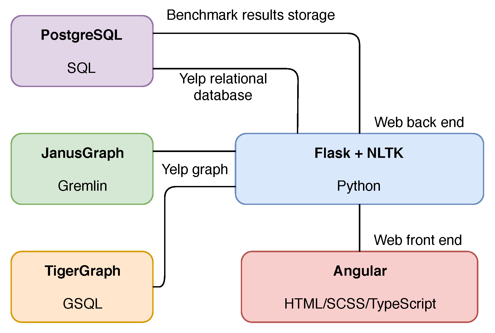
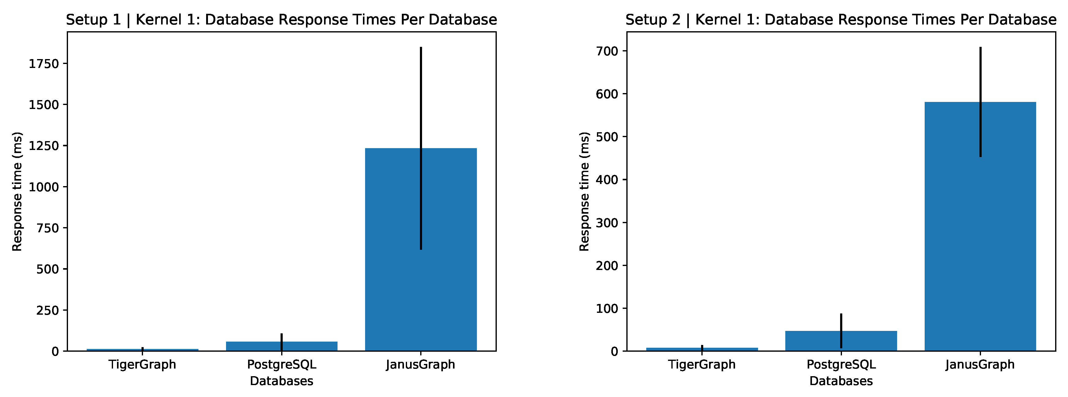
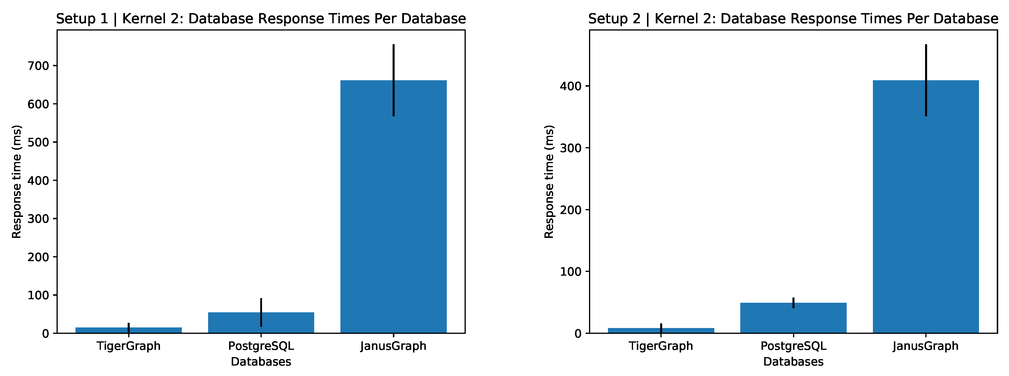
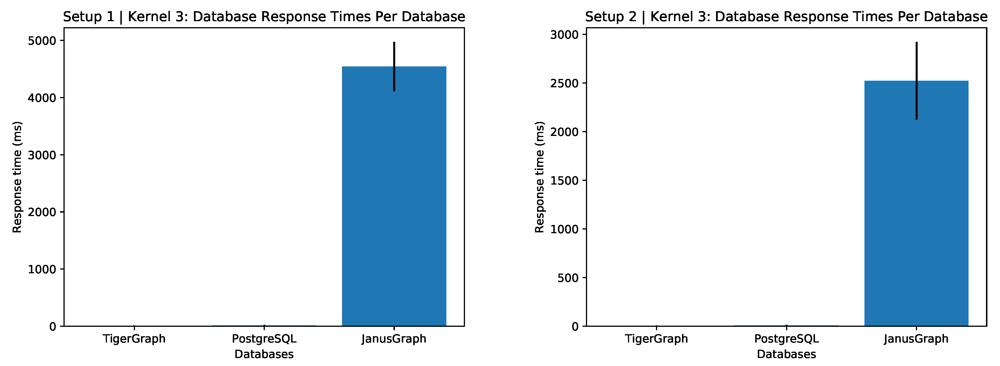
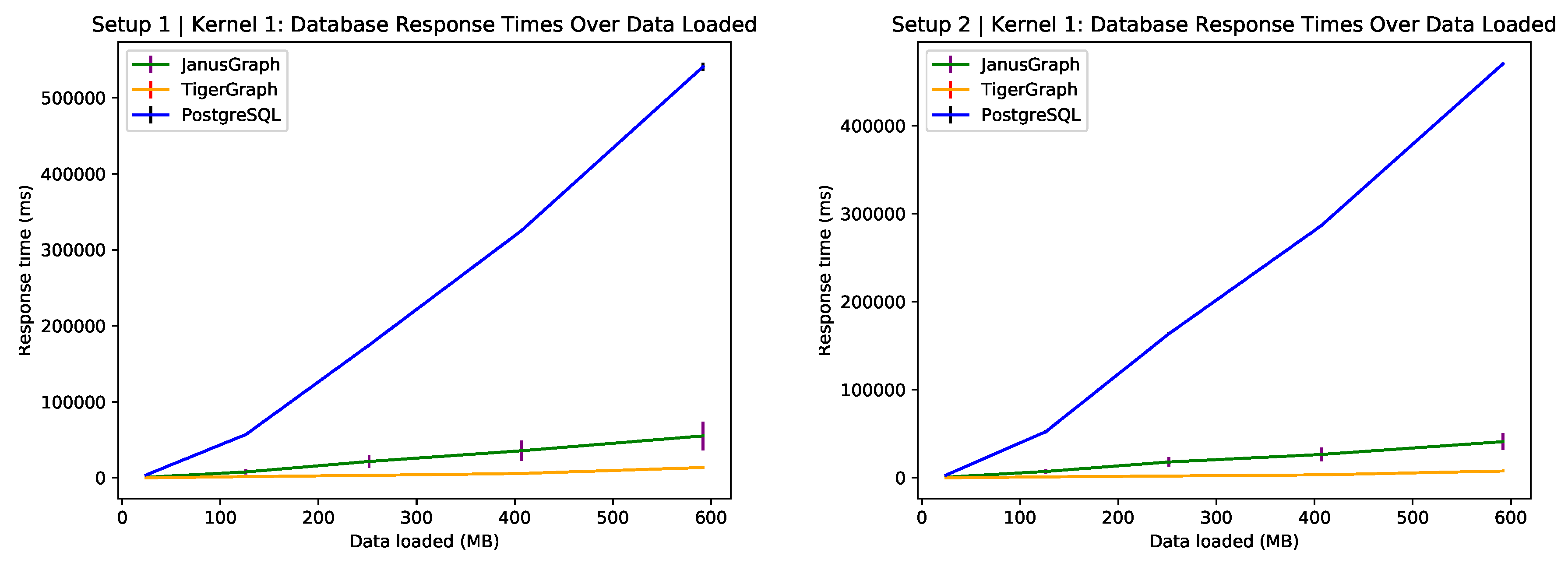
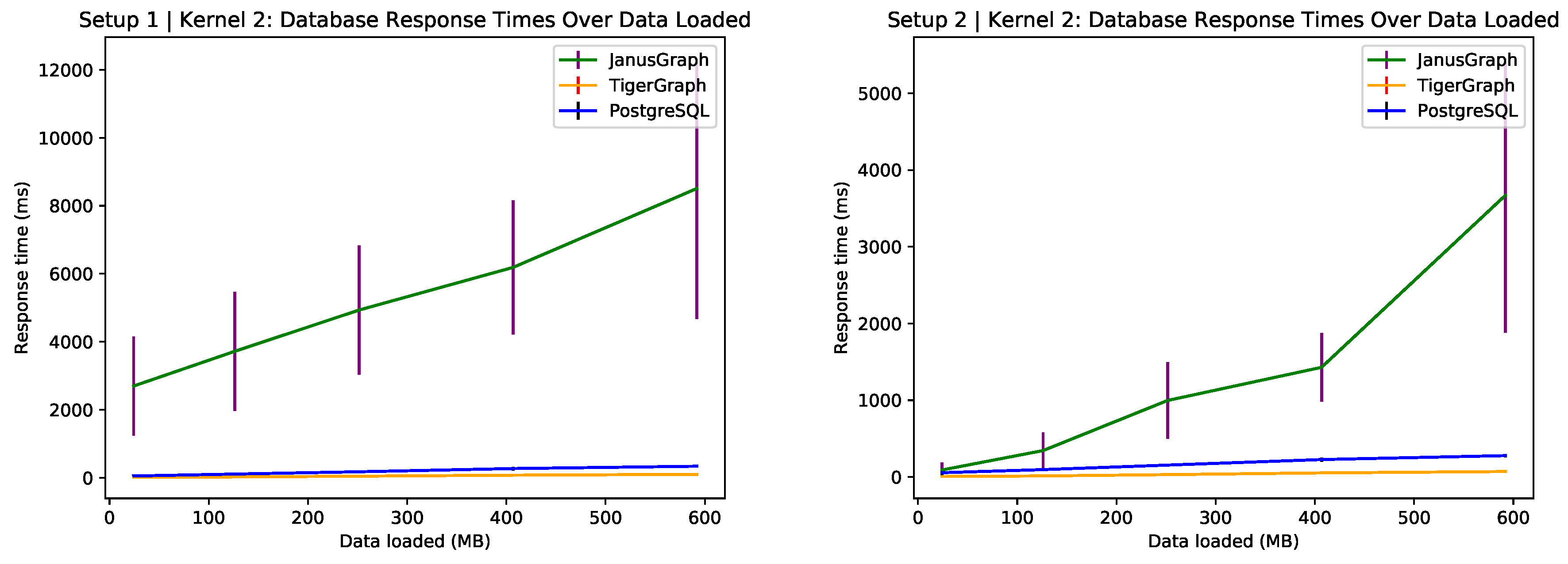
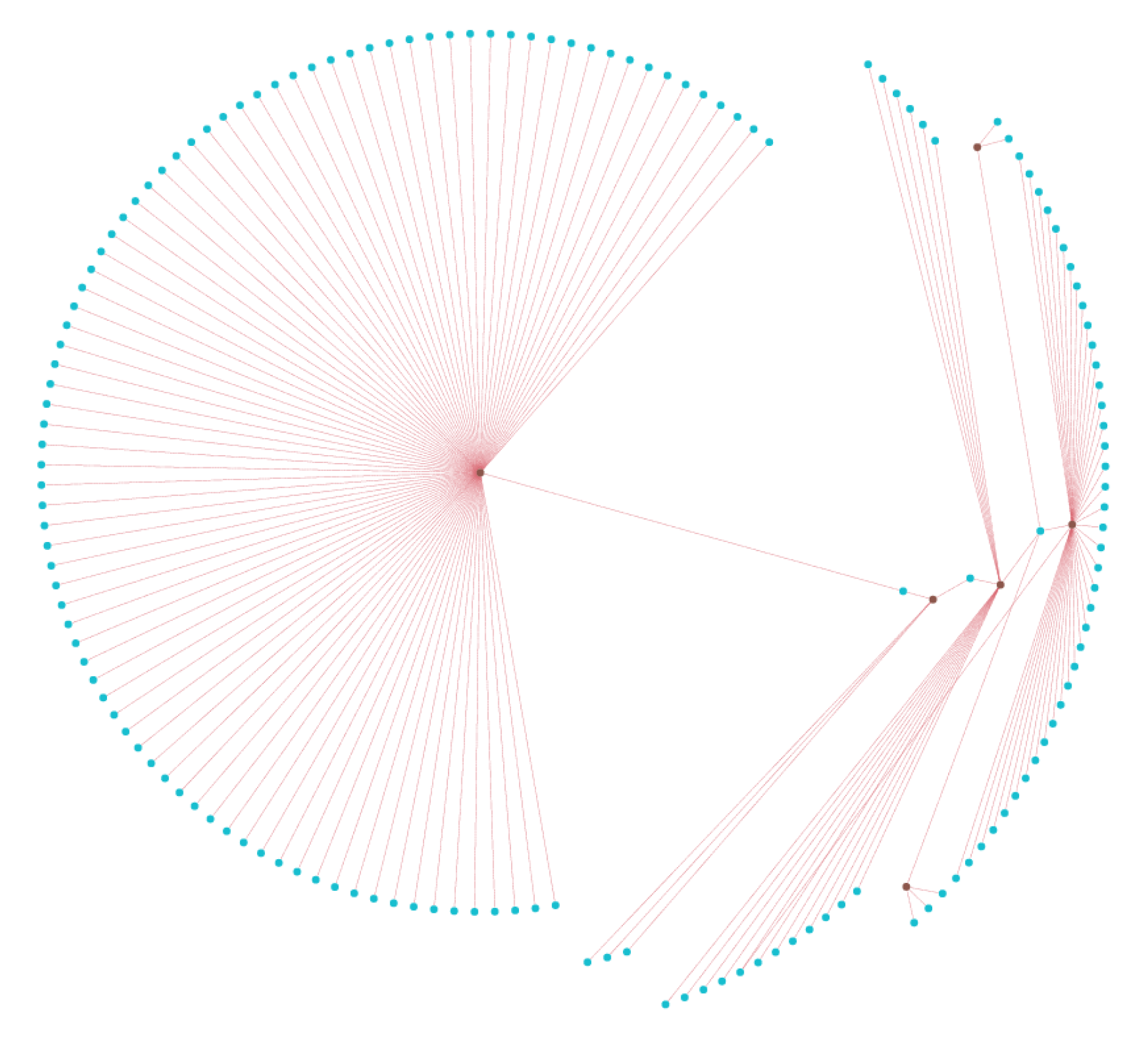
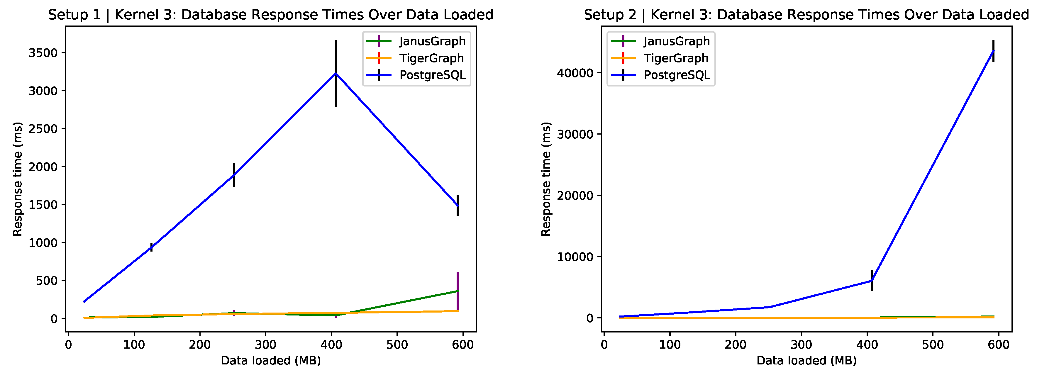
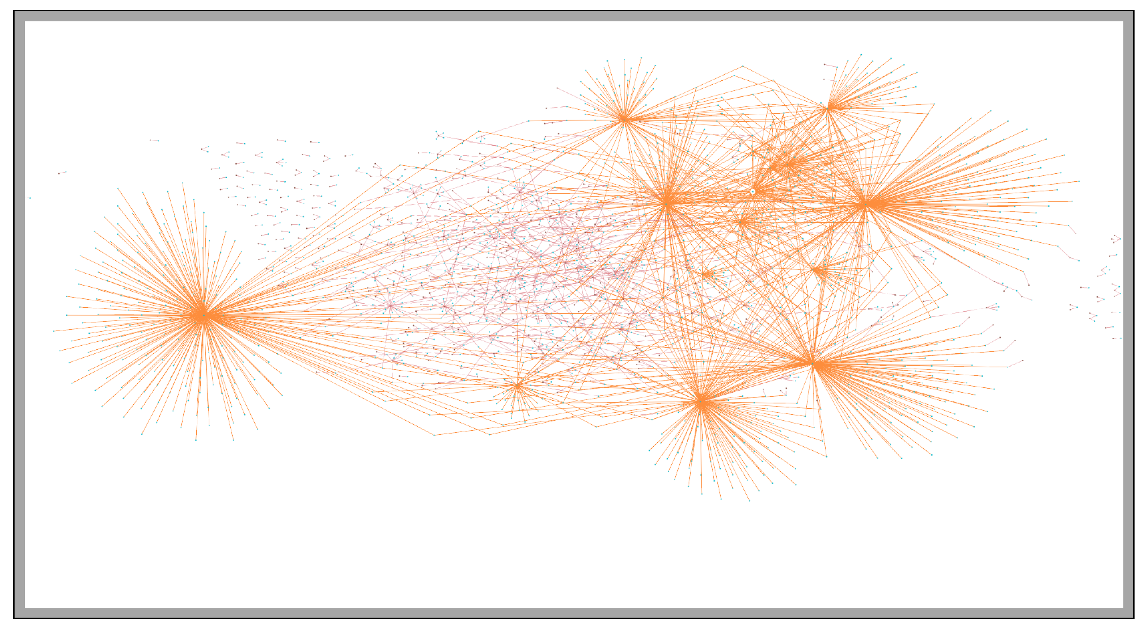
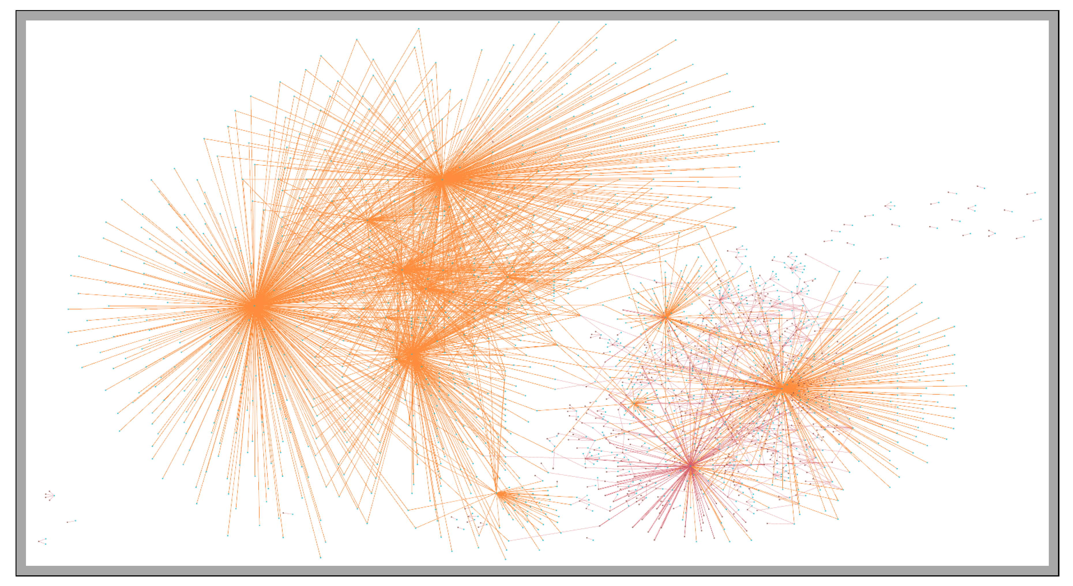
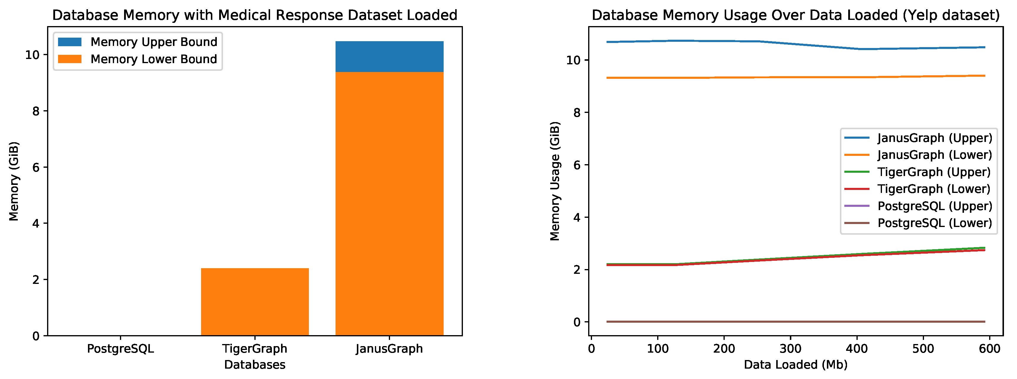
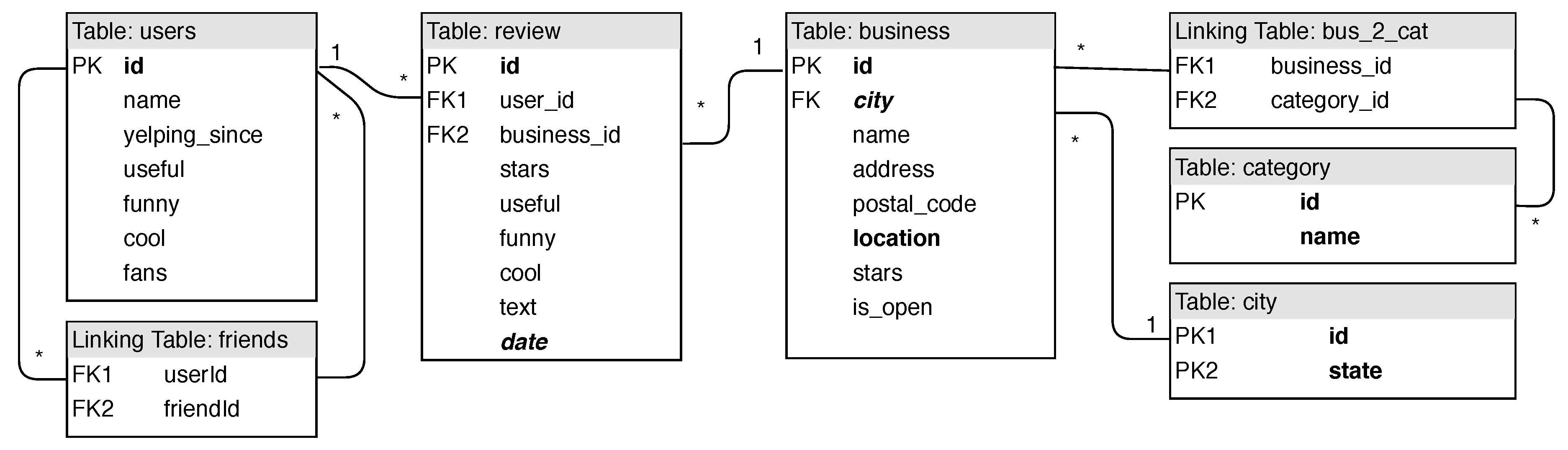
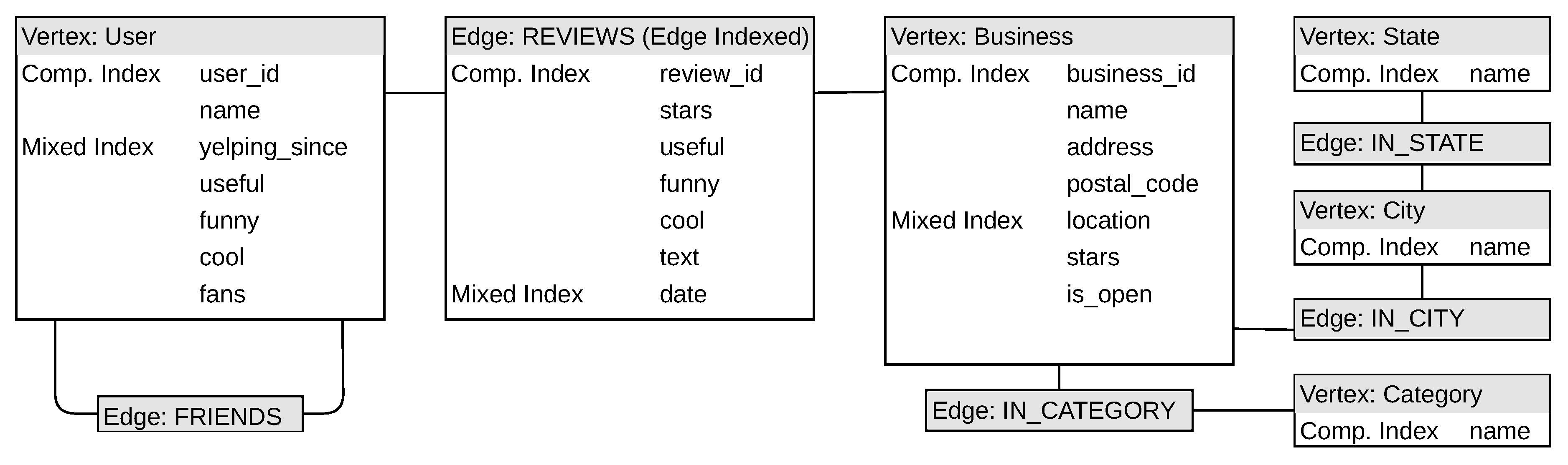
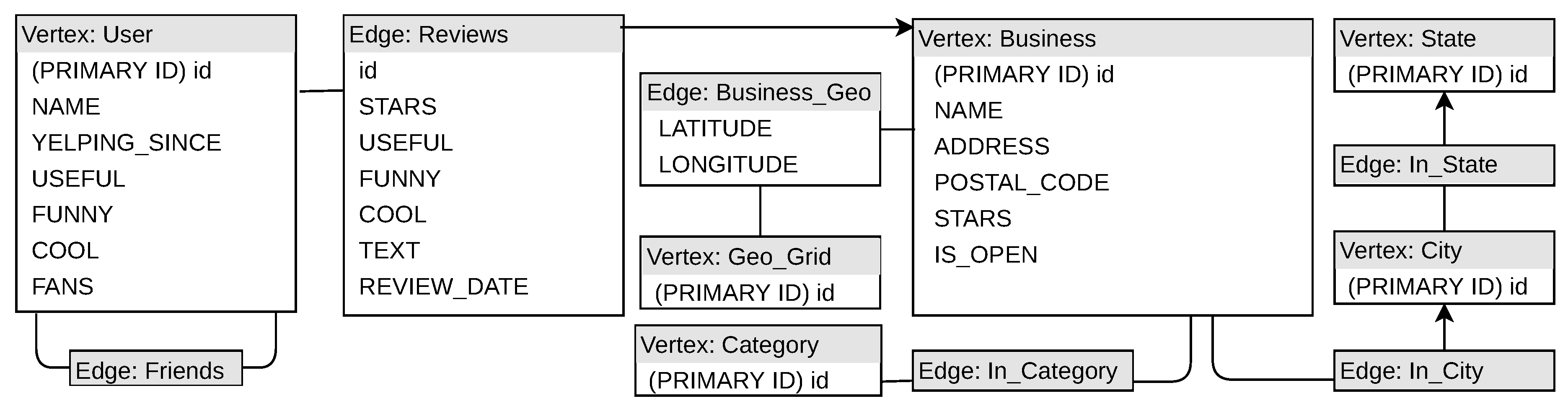
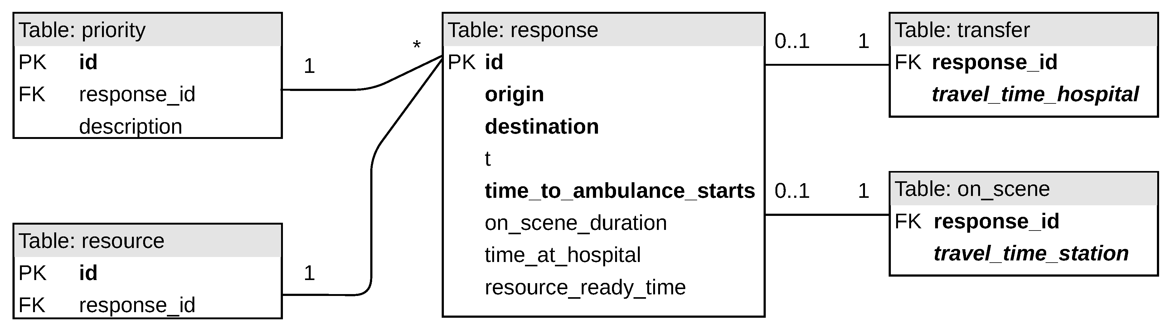
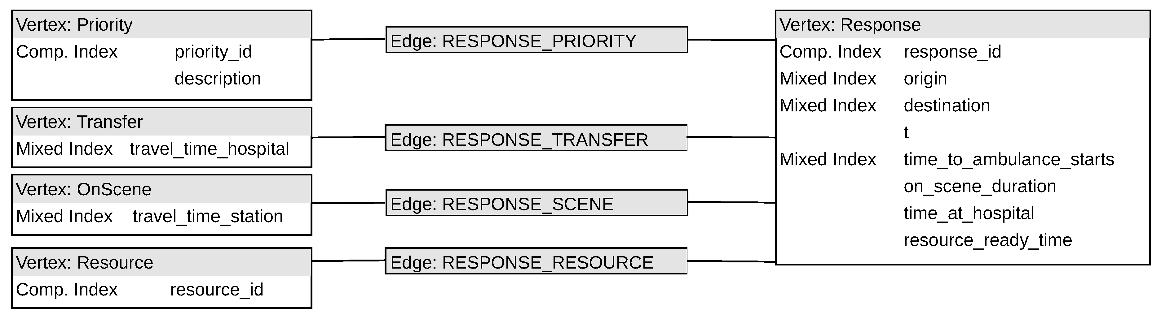
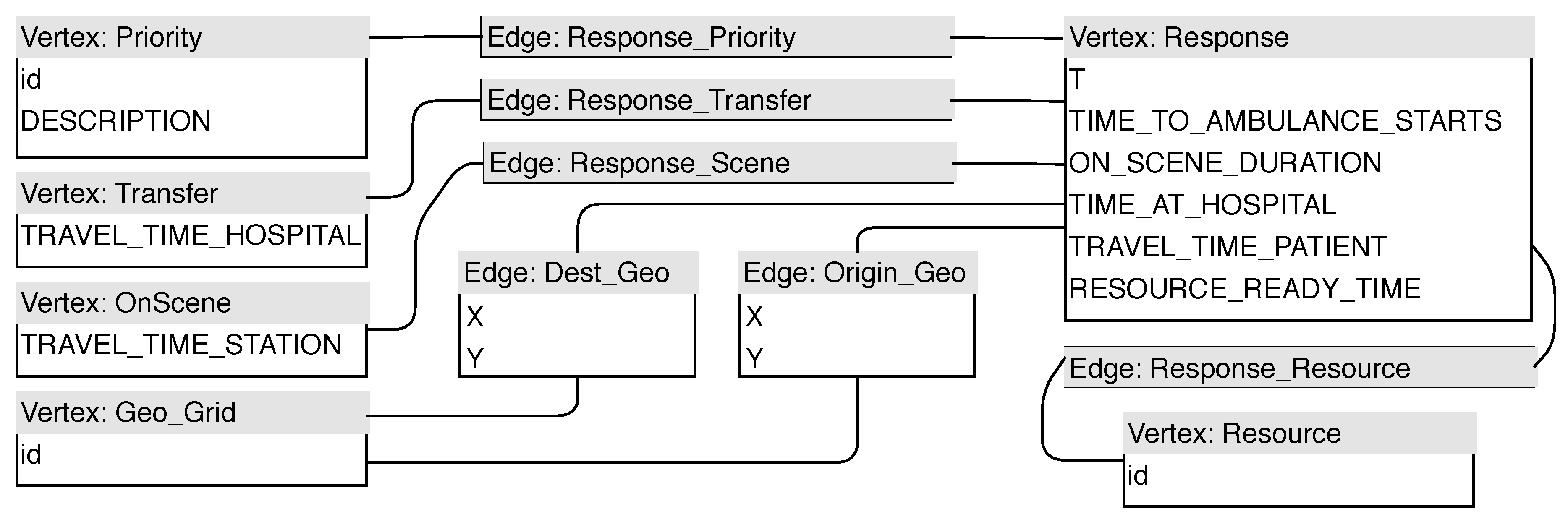
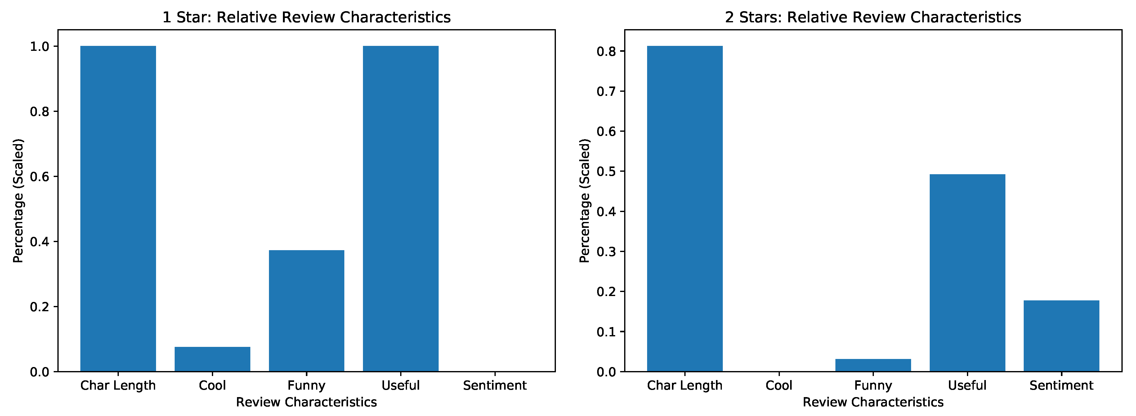
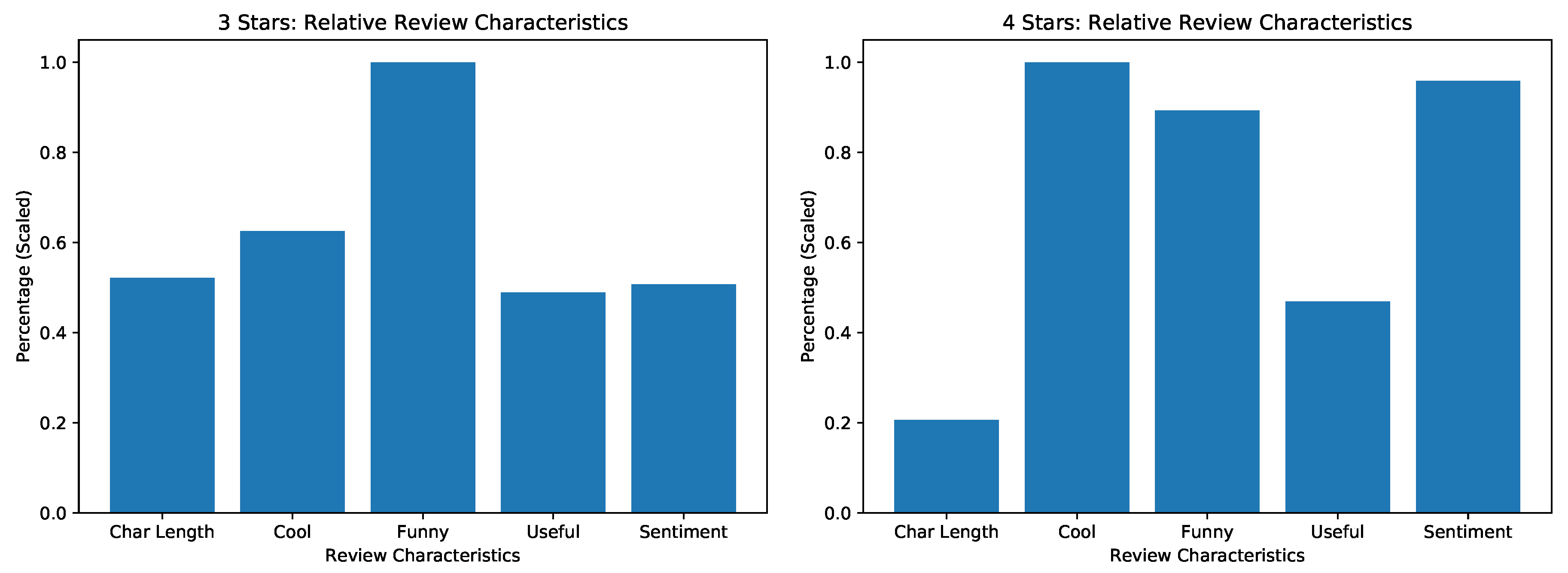
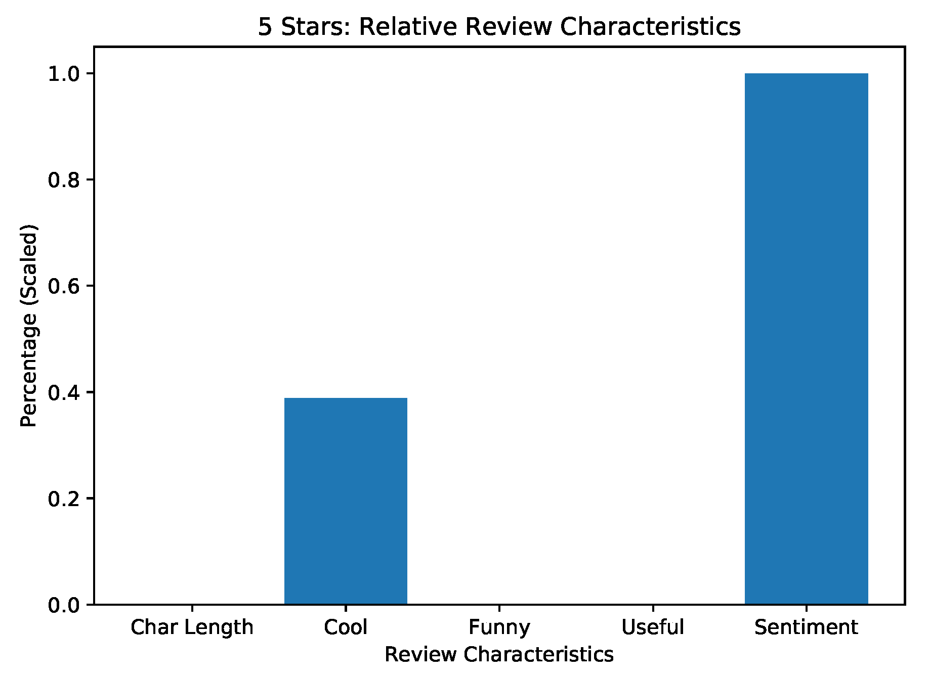


