Internet Video Delivery Improved by Super-Resolution with GAN

Abstract

In recent years, image and video super-resolution have gained attention outside the computer vision community due to the outstanding results produced by applying deep-learning models to solve the super-resolution problem. These models have been used to improve the quality of videos and images. In the last decade, video-streaming applications have also become popular. Consequently, they have generated traffic with an increasing quantity of data in network infrastructures, which continues to grow, e.g., global video traffic is forecast to increase from 75% in 2017 to 82% in 2022. In this paper, we leverage the power of deep-learning-based super-resolution methods and implement a model for video super-resolution, which we call VSRGAN+. We train our model with a dataset proposed to teach systems for high-level visual comprehension tasks. We also test it on a large-scale JND-based coded video quality dataset containing 220 video clips with four different resolutions. Additionally, we propose a cloud video-delivery framework that uses video super-resolution. According to our findings, the VSRGAN+ model can reconstruct videos without perceptual distinction of the ground truth. Using this model with added compression can decrease the quantity of data delivered to surrogate servers in a cloud video-delivery framework. The traffic decrease reaches 98.42% in total.

1. Introduction

Currently, video is the most popular medium for entertainment, communication, and online educational communities. The launch of well-known video services, the advancement of networking technology, and the widespread use of mobile devices were all watershed moments that paved the way for the popularity of online videos. Furthermore, the ability to create and share video content at low cost increased the appeal of video applications, making video the new dominant Internet application.

Internet traffic reports have exposed the considerable amount of bandwidth consumed by such applications and affordable devices capable of playing HD and UHD content, creating scenarios in which this demand will continue into the coming years. Cisco’s annual Internet traffic analysis [1] forecasts that 82% of global traffic will be related to video by 2022 and that 22% will be composed of VoD applications serving HD (57%) and UHD (22%).

The primary source of this traffic is the well-known VoD services, deployed using a multilayer technology solution [2], which deliver a TV-like experience anywhere and anytime. These services embrace adaptive video bitrate technology in the content layer to provide content that matches the audience’s playback resources. In the transport layer, the shortening of playtime [3], i.e., the time between hitting the play button and content screening, happens by using CDNs that serve adaptive bitrate content from the point closest to audiences. In the computing layer, the management of content-access patterns established by large and diverse audiences is achieved by cloud computing.

With the adoption of adaptive bitrate technologies, published videos are encoded to fit a set of screen resolutions and playback bitrates as defined by the targeted audiences. This preprocessing stage happens in the cloud infrastructure, and the output, i.e., a bundle of video files, is moved around through contracted transport infrastructure. Content placement algorithms find the best fit between those files and targeted audiences, subject to strict cost-cutting goals.

All of these efforts are constrained by the practices established in traditional video-publishing workflows, i.e., encoding recipes that set the target resolution and streaming bitrates as output by the end of the encoding phase. Based on these recipes, videos are downward encoded, bundled, and then moved and stored on selected surrogate servers. Moreover, despite all the recent advances in video-compression techniques, moving and storing encoded videos are naturally resource-demanding operations. For instance, a five-second video sequence can demand up to 97 MBytes to store and 156 Mbps to maintain its encoding bitrate during a streaming session that targets HD devices.

A state-of-the-art video workflow implements per-title encoding using machine-learning techniques. These workflows find a set of distinct bitrates that have perceptual meaning to their audiences. In other words, switching from low-bitrate to high-bitrate streaming will improve the video session’s perceived quality. Static-encoding recipes cannot deliver such assurances due to their generality. In [4], the per-title effectiveness was evaluated and showed an impressive 84% savings due to fewer bits per segment and fewer quality changes by the client. However, in such a video workflow, there is a set of encoded videos that require movement and storage to shorten the playtime.

The optimization of Internet video delivery is the subject of many works [2,5,6,7,8], and these cover CDNs, HAS, CDN-P2P, CDN assisted by fog computing, and video SR on the client side, among others. However, video delivery still has many challenges to be solved [2,9]. For example, the amount of video traffic on the Internet has been increasing yearly, heading towards an Internet bottleneck [1,10]. Furthermore, international data traffic provided by Tier-1 ISPs is more expensive than regional and local traffic (Tier-2 and Tier-3 ISPs) [11].

Conversely, the computational power at the edge clouds has increased, which has likewise increased the volume of idle computing resources at the backend servers [12]. In addition, many video-processing tasks can be performed by GPUs, which have gained increased computational power in recent years. This trend in GPU performance has been reducing the processing costs of cloud services [13,14]: e.g., in early 2020, Google Cloud reduced its GPU prices by more than 60% [15].

Using these resources to reconstruct and transcode videos at the edges will relieve the bottleneck that is restricting international Internet traffic in exchange for bringing content and processing closer to the consumers. Moreover, video-delivery and cloud-computing companies could establish a symbiotic business relationship.

Machine learning (ML) has seen an unprecedented boom in applications that address problems and enable automation in a variety of disciplines [16,17]. This is owing to an increase in data availability, significant advances in ML approaches, and breakthroughs in computational capabilities. Recent findings in neural deep learning have provided new venues for publishing videos on the Internet [18,19,20,21,22,23,24,25]. These findings have shown that two neural deep-learning models, CNNs and GANs, can input low-resolution images and upscale them to high resolution [26]. This technique is called image SR, and according to such studies, its output and original images are similar in terms of perceptual quality. These models are the basis of our research, which yields the following contributions:

• We propose a cloud-based content-placement framework that substantially reduces video traffic on long-distance infrastructures. In this framework, low-resolution videos move between servers in the cloud and the surrogate server deployed on the server side. An efficient SR GAN-based model reconstructs videos in high resolution.
• We created a video SR model as a practical solution to use in a video-on-demand delivery system that upscales videos by a factor of 2 with perceptual quality indistinguishable from the ground truth.
• We present a method for mapping the perceptual quality of reconstructed videos to the QP level representation of the same video. This method is essential for comparing the quality of a video reconstructed by SR with the representation of the same video at different compression levels.
• Finally, we evaluate the contribution of SR to reducing the data and compare it with reduction by compression. Additionally, we analyze the advantages of the two approach combinations. Our experiments demonstrated that it is possible to reduce the amount of traffic in the cloud infrastructure by up to 98.42% when compared to video distribution with lossless compression.

We organized this paper as follows. Section 2 discusses works on image and video super-resolution and perceptual video quality metrics. Section 3 presents the video framework proposed in this study. Section 4 offers the proposed SR model and its perceptual loss function. The datasets used to train and test models are presented in Section 5. Section 6 shows the video quality assessment metrics used in this work. The parameters, training details, and numerical results are shown in Section 7. Finally, in Section 8, our conclusions and future work are presented.

2. Background and Related Work

In this section, the body of work on SR using DNNs is presented, followed by studies that evaluate DNN-based SR models for video distribution on the Internet. Finally, we consider a body of work on video quality assessment.

2.1. Super-Resolution Using Convolutional Networks

Image and video super-resolution has gained momentum in different research communities. In recent years, the number of papers published that address the super-resolution problem and appear in qualified conferences and journals has shown an upward trend [26,27]. Combining CNNs, perceptual loss functions, and adversarial training to solve typical SR challenges has fostered this momentum.

Video SR refers to scaling low-resolution frames $f^{LR}\in V^{LR}$ into high-resolution frames $f^{SR}\in V^{SR}$ of video $V_f$, where $f=1,\cdots ,N$, and each frame f has dimensions $W:H:C$, defined by width W, height H, and RGB channel C. $f^{LR}$ are low-resolution frames taken from high-resolution frames $f^{HR}\in V^{HR}$ using a downscaling process defined by a factor r. In the following, we present super-resolution models built to upscale images in the context defined by video.

In [28,29,30], the authors approached the SISR problem using a CNN. The proposed model, called SRCNN, upscales an image using a two-step procedure. The first step scales the low-resolution frame $f^{LR}$ by a bicubic interpolation function to produce $f^Y$, which has the target resolution. The second step uses $f^Y$ to evolve the super-resolution frame $f^{SR}$ to reach the quality measured in the original frame $f^{HR}$. A three-layer CNN performs this quality-evolving process. The main drawback of the SRCNN model is the computational cost associated with the convolution process using an already-high-resolution frame $f^Y$. Despite the smoothing artifacts, which are easily detected by the human vision system, the SRCNN model showed high scores in evaluations using pixel-wise metrics, such as PSNR and SSIM [29].

The model CISRDCNN [31] is a deep convolutional neural-network-based super-resolution algorithm for compressed images. The model is composed of three main blocks. The first part receives low-resolution and compressed images as input, and this part operates to reduce compression artifacts. The second part performs the upscaling operation, and the last part is responsible for quality enhancement and works on the HR image with a considerable computational cost. In addition, the output images show smoothing artifacts.

In [32], the authors introduced the ESPCN model to face constraints due to high-resolution input frames $f^{HR}$. The ESPCN model is a three-layer CNN that performs image up-scaling after the CNN’s third layer in an additional subpixel convolutional layer. Image up-scaling deconvolutes the n layers of features extracted from the low-resolution frame $f^{LR}$. Compared to the SRCNN model, the ESPCN has lower computational demands and similar image quality, although smoothing remains an unresolved issue.

Johnson et al. [33] trained a CNN using a perceptual loss function defined using high-level image features for smoothing the image restoration. The authors use a pre-trained convolutional network to extract those features. Ledig et al. [21] proposed the SRResNet and SRGAN models, which are CNN-based models with 16 RBs. However, the SRGAN model has a perceptual loss function and uses adversarial training. The evaluations of the SRGAN model showed that the perceptual quality of up-scaled images was better than those models based on mean-error loss functions. Its primary drawback is the training instability, which occasionally leads to image artifacts due to BN, a deep-learning training technique that is broadly applied to the image classification task.

Wang et al. [22] proposed the ESRGAN model. It has residual scaling, 23 RRDBs, and a RaD. The latter measures the probability that the generated data are more realistic than the actual data and vice versa. This model helps build fast and stable training sessions and improves the images’ perceptual quality. The ESRGAN model is the state-of-the-art SISR technique. However, the model’s dense and deeper architecture shows a prohibitive computing cost for up-scaling HD and 4K videos in real applications.

In recent years, several multi-frame super-resolution methods [34,35,36,37,38,39] have manifested higher performance compared with SISRs. Multiframe-based methods explore temporal information from neighboring frames in addition to spatial information. In other words, exploring temporal information means that these methods include multiple frames as input to the neural network. To our knowledge, there are no practical solutions for videos with multiple scene changes in the multi-frame super-resolution model.

The proposed multi-frame super-resolution methods have been tested with video datasets [40,41,42,43] that present sequential frames recording movements in static background scenarios. In addition, such methods have been tested in low-resolution video datasets since they have a higher computational cost. This cost comes from the convolutional layer designed to receive multiple input images. Moreover, this convolution requires considerable memory for HD videos, which causes frequent GPU memory overflows. In this paper, we assume that videos are HD and FHD encoded with frequent changes in the background scenario. Therefore, our method is SISR-based and does not explicitly explore temporal information.

This paper proposes a novel SR model assuming that a cloud-based video service manages all super-resolved videos. The built model, called VSRGAN+, has a low computational cost compared to the state-of-the-art approaches and is an improved version of our previous VSRGAN model [44]. The primary enhancement in VSRGAN+ is the introduction of RRDBs, a new perceptual loss function, and a RaD as shown in Section 4. This enhancement enables the generation of sharper images compared with the previous model VSRGAN.

Table 1. The main characteristics of SR-related models.

Models	CNN	Sub- Pixel	RB	RRDB	Skip Connection	Perceptual Loss	GAN	Dense Skip Connections	RaD	Residual Scaling	Video SR
SRCNN [28]	√	✕	✕	✕	✕	✕	✕	✕	✕	✕	✕
ESPCN [32]	√	√	✕	✕	✕	✕	✕	✕	✕	✕	√
CISRDCNN [31]	√	✕	✕	✕	√	✕	✕	✕	✕	✕	✕
SRResNet [21]	√	√	16	✕	√	✕	✕	✕	✕	✕	✕
SRGAN [21]	√	√	16	✕	√	√	√	✕	✕	✕	✕
ESRGAN [22]	√	√	✕	23	√	√	√	√	√	√	✕
VSRGAN [44]	√	√	3	✕	√	√	√	√	✕	✕	√
VSRGAN+ (ours)	√	√	✕	3	√	√	√	√	√	√	√

shows the main characteristics of each SR-related model described in this section. We present the proposed model in Section 4.

2.2. DNN Super-Resolution for Internet Video Delivery

In [9], the authors addressed the challenges of Internet video delivery by running DNN-based super-resolution models on the client side. On the server side, videos were clustered based on their content and encoded at low resolution. In each cluster, a DNN-based super-resolution model was proposed and served along with each video. On the client side, the built DNN model super-resolves the delivered content and creates a streaming session at the expense of transmitting low-resolution content and running a DNN model. The principal assumption was that client devices have the resources to run a DNN model in a feasible time window.

In [6], the authors considered a bitrate adaptive streaming session as the input of the DNN-based super-resolution model proposed in [9]. The rationale was to super-resolve low-resolution segments that arrive during the session and decrease the computing burden of super-resolving all video segments. The authors chose a state-of-the-art adaptive bitrate algorithm to control the quality of the streaming session. Experimental studies showed perceptual improvements using super-resolution models compared to streaming sessions performed without these models.

These two papers super-resolved videos on the client side, in contrast to the approach taken herein. We use super-resolution models in the surrogate servers of a cloud-based video service, intending to overcome the computing deficit on the client side while, at the same time, reducing the traffic between video injection points and surrogate servers.

2.3. JND-Based Video Quality Assessment

The JND is the difference between two signals at the threshold of detectability[45]. It is applied to understand the sensitivity of the human visual system. In [46], the author introduced the JND concept as a metric for measuring video quality. In [47], the author proposes an interactive JND-based method to establish the encoding bitrate of consecutive video representation, which makes encoding distortions noticeable to the human eye. A dataset of encoded videos using this method was created and presented by [48]. This dataset includes 220 videos with four resolutions and 52 encoding representations. By applying the JND methodology, three JND points per resolution were defined, showing the inefficiency of video encoding in the 52 range.

In [49], the authors presented a metric called LPIPS, which measures the perceptual distance between two images. The extraction of features uses a deep neural network and defines the LPIPS values. The authors compared the LPIPS and JND outcomes to conclude that there is a strong correlation between the extracted features and the artifacts that catch the attention of the human visual system.

In this work, we use the dataset presented in [48] to conduct experimental studies. Moreover, a novel method is presented based on the LPIPS metric mapping JND points of super-resolved videos.

3. Cloud-Based Content Placement Framework

Well-known video-streaming services, for instance, Netflix and Hulu, use a CDN to improve the QoE of video sessions by reducing the delay and increasing the throughput. CDNs use two architectures: enter deep and bring home [50]. The first architecture penetrates the ISPs deeply by placing content distribution servers in the ISP PoPs. The second architecture brings ISPs closer to their customers by concentrating massive content distribution centers in a few critical areas and linking them with private high-speed connections.

Due to today’s audience segmentation of video-streaming services, the CDN content placement policies deployed on those architectures require moving large quantities of data to multiple surrogate servers, which are the audience’s closest access points. The cost of approximating content and its audience is the transmission cost. IaaS, one of the cloud-computing-service models, has been used to address the natural fluctuations in computing resource demands for those operations. Despite the advantages of the pay-as-you-go pricing of the IaaS model, there are costs associated with moving large files around the Internet, e.g., the congestion of dedicated links and increases in the time to market.

In this paper, we propose a content-placement framework for reducing the quantity of data delivered between the source server and surrogate servers. This framework can support VoD streaming services using both CDNs enter-deep and bring-home architectures. Figure 1 shows the content-placement framework considered in this work.

In this framework, the super-resolution procedure starts after the content placement policy establishes which video V has to be stored on the surrogate server S. The high-definition version of selected video V, $V^{HR}$, is stored in the original server and encoded to output its low-definition representation $V^{LR}$. This downscaling process reduces the actual scenes by a factor of r.

The low-resolution representation is replicated in the surrogate servers, in contrast to the all-version approach. The DNN runs a factor r procedure to upscale that representation in surrogate servers. This procedure’s output is served as mono-bitrate video sessions or is involved in the multi-bitrate publishing workflow.

We designed this framework for VoD streaming services, and thus the SR tasks are performed offline and run based on a pre-established schedule. Additionally, we assume that surrogate server GPUs have the computing resources to complete the SR tasks using a parallel-processing model.

The Video-Size Optimization Problem

Problem and Goal. To pursue a high level of engagement, video services must deal with audience fragmentation. These services have to move and store a large amount of data to surrogate servers close to the audience to keep the QoE of video sessions at high levels, i.e., reduced delay and suitable streams. In this scenario, the cost of moving the video content is highly affected by the size of the encoded videos. Hence, the challenge is in solving the trade-off between decreasing the media size to be moved, consequently lowering the operating costs, and keeping the QoE at a high standard.

In the following, we present the formulation of this challenge, which is a video-size minimization problem involving the QP and video resolution subject to a quality threshold (Equation (1)).

$$\begin{array}{cc}\hfill & \underset{q,p}{min}\sum _i^{K}Siz{e}_{V_i^{LR}}\left(q,p\right)\hfill \\ \hfill s.t.& VQ\left(DNN\left(V^{LR}\right)\right)-VQ\left(V^{HR}\right)⩽V{Q}_T\hfill \\ \hfill & \forall i,q\in \left\{0,\cdots ,51\right\}\hfill \\ \hfill & \forall i,p⩽V_T^{LR}\hfill \end{array}$$

(1)

where $Siz{e}_{V_i^{LR}}$ is the size of the low-resolution video i (in bytes). K is the number of videos involved in the operation. The quality of DNN-based super-resolved videos is $VQ\left(DNN\left(V^{LR}\right)\right)$, the quality of the ground truth videos is $VQ\left(V^{HR}\right)$, and the threshold of the target quality degradation is $V{Q}_T$. q and p are the QP and the resolution of low-quality videos, respectively. The aspect ratio of the low-quality video is 16:9. $V_T^{LR}$ is the threshold of the low-resolution video.

Approach. The $DNN(.)$ model is trained to satisfy a threshold of levels of compression artifacts and defines the quality threshold restriction. Finding the optimal solution is unfeasible because changes in the artifact levels require the DNN model updating. Thus, we address this problem using JND as a threshold for $V{Q}_T$ based on studies presented in [48] for an extensive video dataset.

4. Video Super-Resolution with GAN

This research assesses the video super-resolution technique to address the delivery of high-quality video content. More specifically, in the context of a cloud-based video service, a super-resolution model is utilized to lower the cost of conventional methods that address end-to-end network congestion. The SR model is a generative adversarial network, i.e., a deep-learning model for image up-scaling that super-resolves sharper and more realistic images [19,22]. We named the proposed model improved Video Super-Resolution with GAN (VSRGAN+) and present it in the following subsections.

4.1. VSRGAN+ Architecture

The adversarial network architecture includes a generator network $G\left(f^{LR}\right)$ and a discriminator network $D\left(G\left(f^{LR}\right)\right)$, which compete against each other during training. $G(.)$ learns how to generate frames, $f^{SR}$ that are indistinguishable from the ground truth frames, expecting to go undetected by $D(.)$. $D(.)$ learns how to distinguish the generated frames from the ground-truth frames. In other words, adversarial training works to balance these two dynamics.

In [51], the authors classified adversarial networks as a min–max problem. In this work, we use this classification to define an adversarial network for video super-resolution as follows:

$$\begin{array}{cc}\underset{{\theta }_G}{\min }\underset{{\theta }_D}{\max }V(D_{{\theta }_D},G_{{\theta }_G})=& \\ & f^{HR}\sim p_{train}\left(f^{HR}\right)\left[log{D}_{{\theta }_D}\left(f^{HR}\right)\right]+\hfill \\ & f^{LR}\sim p_G\left(f^{LR}\right)\left[log\left(1-D_{{\theta }_D}\left(G_{{\theta }_G}\left(f^{LR}\right)\right)\right)\right],\hfill \end{array}$$

(2)

where we train the discriminator network $D_{{\theta }_D}$ to maximize the probability of its outcomes correctly classifying both frames: the ground-truth and the super-resolved frames. The generator network $G_{{\theta }_G}$ learns how to generate more realistic frames $f^{{}_{SR}}$ by tuning the parameters ${\theta }_G$ to minimize $log\left(1-D_{{\theta }_D}\left(G_{{\theta }_G}\left(f^{LR}\right)\right)\right)$, where ${\theta }_G=\{W_{1:L};b_{1:L}\}$. W are the weights, and b is the bias of the L-layer neural network that is optimized by a loss function $L_G$ during training.

During the generator network training sessions, we use a set of frames, $f_i^{LR}$, encoded at a low bitrate, and their counterparts $f_i^{HR}$, subject to the minimization of the following loss function.

$$\begin{array}{c}\hfill {\theta }_G=arg\underset{{\theta }_G}{min}\frac{1}{N}\sum _{i=1}^N{L}_G\left(G_{{\theta }_G}\left(f_i^{LR}\right),f_i^{HR}\right)\end{array}$$

(3)

where $L_G$ is the generic function that computes the loss between the super-resolved image and the ground truth image; in Section 4.2, this loss function is presented in detail.

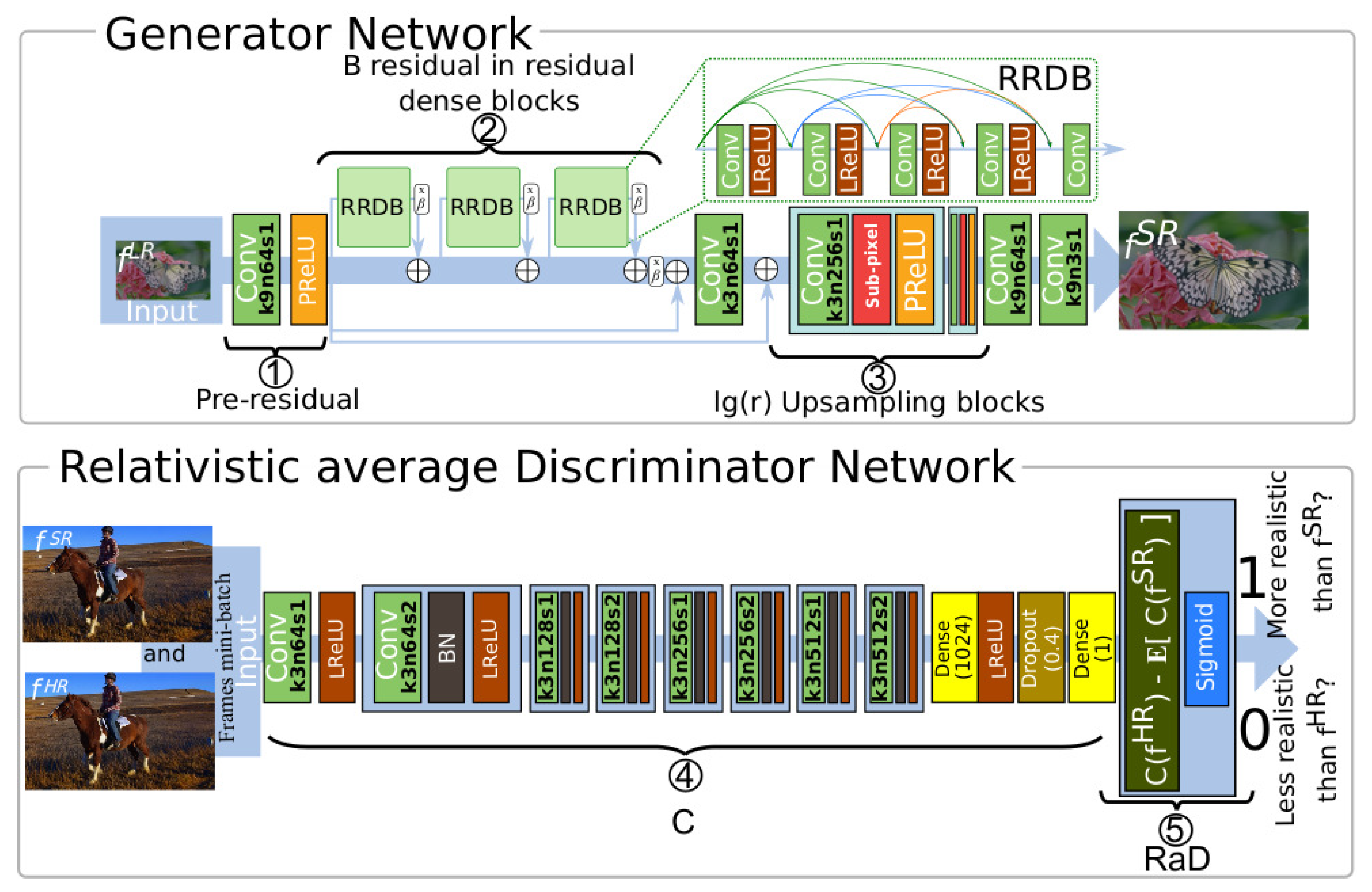
The generator network has a pre-residual block (part 1) containing a convolution layer (k9n64s1)—namely, 64 filters sized $9\times 9$ and one stride, and the PreLu activation function [52]. The core of the generator network (part 2) has B residual-in-residual dense blocks (RRDBs) [22] with dense skip connections. Each RRDB has five convolution layers, with this k3n64s1 setup followed by the activation LeakyReLU [53]. At the output of each RRDB, there is a residual scaling $\beta$ [54].

After the RRDBs, there is a residual scaling value $\beta$, a skip connection from the pre-residual block, and a convolution layer set as k3n64s1, followed by another pre-residual skip connection.

For upscaling resolution, $G(.)$ has ${log}_2\left(r\right)$ blocks (part 3), where r is the scaling factor, which is a multiple of 2. Each block has a convolution layer set as k3n256s1, followed by a SubpixelConv2D and PReLU [32]. Finally, the last part of $G(.)$ has two convolution layers, set as k9n64s1 and k9n3s1.

The discriminator has two parts, C (part 4) and RaD (part 5). C consists of convolution k3n64s1, followed by an activation LeakyReLU with $\alpha =0.2$. The core of C has seven blocks composed of a convolution layer, a BN layer, and LeakyReLU activation with $\alpha =0.2$. The convolution layer of the first block consists of k3n64s2. The other blocks conduct convolution with three sizes of filters; the number of filters varies for each pair of blocks in 128, 256, and 512, with the first pair having one stride and the second having two strides. The final part of C includes a dense layer with 1024 neurons, LeakyReLU activation, dropout of 40%, and a dense layer with only one neuron.

Generally, a standard discriminator, D, is used to calculate the probability of a realistic frame. This discriminator is defined by $D\left(f^{SR}\right)=\sigma \left(C\left(f^{SR}\right)\right)$$\forall f^{SR}$ and $D\left(f^{HR}\right)=\sigma \left(C\left(f^{HR}\right)\right)\forall f^{HR}$, with C being the output of the discriminator before $\sigma$ activation. We chose a different approach to accomplish this; we used a relativistic average discriminator (RaD).

Figure 2 (part 5) presents the applied RaD, described in [55]. The RaD function uses the information coming from the C component, i.e., $RaD(f^{HR},f^{SR})=\sigma (C\left(f^{HR}\right)-\mathbb{E}\left[C\left(f^{SR}\right)\right])\forall f^{HR}$ and $RaD(f^{SR},f^{HR})=\sigma (C\left(f^{SR}\right)-\mathbb{E}\left[C\left(f^{HR}\right)\right])\forall f^{SR}$, where $\mathbb{E}[.]$ represents the C output average for all frames in a minibatch. In other words, the $RAD(.)$ gives the probability that $f^{HR}$ is relatively more realistic, on average, compared with a random sample of $f^{SR}$ and vice versa. The use of RaD helps the generating network learn how to super-resolve sharper images [22].

4.2. Perceptual Loss Function

In [56], the authors proposed mean-based loss functions that generate good quality pixel-wise images, according to PSNR and SSIM. However, the human eye quickly detects the smoothing artifacts of these images. In other words, mean-based loss functions are insufficient to capture human visual perception, which has inspired a new body of work on perception-oriented loss functions; see [21,22,33,57,58].

In [21,22,33], the authors proposed a perceptual loss function that has three components: (i) the perceptual component, (ii) the adversarial component, and (iii) the content component; see Equation (4).

$$\begin{array}{c}\hfill L_G=L_{percept}+\lambda L_G^{RaD}+\eta L_1\end{array}$$

(4)

The calculation of the perceptual loss component ($L_{percept}$) uses the mean-error loss defined by the space established using features extracted from the super-resolved frames $f^{SR}$ and their high-resolution counterparts $f^{HR}$. These features are the output of an image classification procedure of VGG19; a deep neural network presented by [59]. This feature classification occurs at the fifth block before the activation function in the fourth convolution layer of the VGG19, called $VG{G}_{54}$. The coefficients $\lambda$ and $\eta$ weigh each component.

Equation (5) presents the perceptual loss component.

$$\begin{array}{c}\hfill L_{percept}=\frac{1}{W.H}\sum _{x=1}^W\sum _{y=1}^H{\left(VG{G}_{54}{\left(f^{HR}\right)}_{x,y}-VG{G}_{54}{\left(f^{SR}\right)}_{x,y}\right)}^2,\end{array}$$

(5)

where W and H are the dimensions of the feature space.

The adversarial loss component $L_G^{RaD}$ is a cross-entropy function as given by Equation (6).

$$\begin{array}{cc}\hfill L_G^{RaD}=& -{\mathbb{E}}_{x_r}\left[log\left(1-D_{RaD}(x_r,x_f)\right)\right]\hfill \\ \hfill & -{\mathbb{E}}_{x_f}\left[log\left(D_{RaD}(x_f,x_r)\right)\right],\hfill \end{array}$$

(6)

where $x_r=f^{HR}$ and $x_f=G\left(f^{LR}\right)$.

The content loss component ($L_1$) is given by Equation (7)

$$L_1=\frac{1}{WH}\sum _{x=1}^H\sum _{y=1}^W\left|f_{x,y}^{HR}-G{\left(f^{LR}\right)}_{x,y}\right|,$$

(7)

where W and H are the dimensions of $f^{HR}$.

5. Datasets

Two datasets are considered for training and testing the proposed models in this work. The first is a high-definition image dataset used to train the proposed models. The second is a video dataset used to test the models. Due to its diversity of scenarios, the first dataset demonstrated excellent fitting for training the models. It includes 1.8 million images from 365 categories in the training set; and 36,500 images, 100 per category, in the validation set. In [60], the authors presented and named this dataset as Places365-Standard.

The dataset of videos has 220 five-second video clips, each with four resolutions: 1080p, 720p, 540p, and 360p. This range of video resolutions targets the prevalence of 1080p and 720p in video-streaming applications for widescreens, e.g., smart TVs and laptops, and the prevalence of 540p and 360p in video-streaming applications for small screens, e.g., smartphones and tablets. This dataset was presented in [48] and is called VideoSet.

H. 264/AVC encoded all clips in the color space YCbCr4:2:0, and QP in [0; 51]. $QP=0$ indicates that the videos are losslessly encoded, and $QP=51$ means that the videos have the highest compression ratio, which shows the highest (lowest) bitrate and best (worst) image quality per frame, respectively.

In [48], 30 subjects evaluated the video quality of all pieces of the VideoSet. Each subject watched encoded videos and identified three JND points, splitting the encoded videos into four sets, with $Q_1$ presenting the best-perceived quality and $Q_4$ the worst quality. The QP values range in $[7,47]$; hence, encoded videos with QP in $[0,6]$ have unperceived quality changes, and those with QP in $[48,51]$ have unacceptable quality.

$$Q_i=\left\{\begin{array}{cc}{Q}_1\hfill & \mathrm{if}Q{P}_{V_i}<Q{P}_{1^{st}JND\in V_i}\hfill \\ Q_2\hfill & \mathrm{if}Q{P}_{1^{st}JND}⩽Q{P}_{V_i}<Q{P}_{2^{nd}JND\in V_i}\hfill \\ Q_3\hfill & \mathrm{if}Q{P}_{2^{nd}JND}⩽Q{P}_{V_i}<Q{P}_{3^{rd}JND\in V_i}\hfill \\ Q_4\hfill & \mathrm{if}Q{P}_{V_i}⩾Q{P}_{3^{rd}JND\in V_i}\hfill \end{array}\right.$$

The VideoSet comprises five-second clips sampled from videos of various subjects.

Table 2. VideoSet’s content and quality.

Title	# of 5 s Samples	Quality (FPS)
El Fuente	31	30
Chimera	59	30
Ancient Thought	11	24
Eldorado	14	24
Indoor Soccer	5	24
Life Untouched	15	30
Lifting Off	13	24
Moment of Intensity	10	30
Skateboarding	9	24
Unspoken Friend	13	24
Tears of Steel	40	24

shows the video titles, the number of samples, and the number of FPS of each sample.

The general conclusion is that VideoSet’s contents and qualities are representative samples of the available content in today’s video service. For instance, the title Tears of Steel is a cartoon-like action movie, El Fuente is a TV-like drama series, and Unspoken Friend is a 90-min movie. All of this content is encoded to target multiscreen audiences.

6. Video Quality Assessment Metrics

We used three metrics to assess the quality of super-resolved videos. The first metric is pixel-wise, i.e., looking to the pixels to determine the quality. The other two are perceptual-wise, i.e., attempting to mimic the human visual system in perceiving quality.

6.1. Pixel-Wise Quality Assessment

The peak signal-to-noise ratio (PSNR) assesses the quality of videos, calculating the ratio of the maximum value of a signal and the power of distortion noise in decibels. The PSNR highest value indicates the best video quality; see Equation (8).

$$PSNR=\frac{1}{N}\sum _{i=1}^{N}20{log}_{10}\frac{max\left(f_i^{HR}\right)}{\sqrt{MSE(f_i^{HR},f_i^{SR})}},$$

(8)

where N is the total number of frames. The MSE is given by

$$MSE=\frac{1}{WH}\sum _{x=1}^H\sum _{y=1}^W{\left(f_{x,y}^{HR}-f_{x,y}^{SR}\right)}^2,$$

(9)

where W and H are the dimensions of the frames.

Although the PSNR inconsistently captures human visual perception [21,61], it has been applied to the video quality assessment revealing the difference between the two signals.

6.2. Perceptual Quality Assessment

Assessing video quality through human vision/audience feedback is desirable but costly. However, a body of qualitative assessment works has been developed based on the mechanisms of human vision. In the following, we present two perceptual metrics.

6.2.1. Learned Perceptual Image Patch Similar—LPIPS

The LPIPS [49] assesses the perceptual distance between the distorted and original videos. Zero-distance means that two videos are perceptually equivalent. This distance assessment uses a space established by high-level video features. For building this space, deep neural networks, conceived to image classification, are used to identify and extract those features, namely: VGG [59], SqueezeNet [62], and AlexNet [63].

In this work, we built the LPIPS feature space using SqueezeNet due to its reduced computational cost and similar outcomes compared to VGG and AlexNet as shown in [49]. In the same work, the authors showed that these three networks learned world representations related to perceptual judgments. Therefore, the LPIPS strongly correlates with human perceptual metrics, such as JND. Moreover, the LPIPS generalizes different distortions, including those streamed by the SR algorithms.

6.2.2. Video Multimethod Assessment Fusion—VMAF

The VMAF [64,65] correlates subjective evaluations to determine the quality perceived by human vision. It assesses the quality of the distorted video and its ground truth in a two-step procedure. First, it computes elementary metrics for both videos and fuses all calculated values in the first step through an SVM regression. The VMAF final score ranges from zero to 100, with a score of 100 indicating perceptual similarity between the two videos. The video streaming industry has used VMAF, i.e., Netflix (https://medium.com/netflix-techblog/vmaf-the-journey-continues-44b51ee9ed12, accessed on 19 April 2022), supported by its strong correlation with perceptual evaluations.

7. Experimental Results

This section presents the results of a large body of numerical experiments. Section 7.1 shows the parameters and training details of the SR models. After that, we assess the video quality using qualitative and pixel-wise metrics. Section 7.3 presents evidence that the human system lacks accuracy, as it only detects significant image distortions.

Additionally, we show that the human visual system perceives the SR videos and their ground truths as similar. In Section 7.4, we analyze the trade-offs brought by the processing time and the video quality. Finally, we examine the improvements that video super-resolution brings to content replication policies deployed by cloud-based video services, subject to setup concerning the video-encoding rate and resolution.

7.1. Model Parameters and Training

The training of models used a high-definition image dataset and a server with GPU NVIDIA GeForce GTX 1080Ti-11GB, CPU i7-7700, 3.60 GHz, and 62 GB RAM. The testing used a laptop with GPU NVIDIA GeForce GTX 1070Ti-8GB, CPU i7-8700, 3.20 GHz, and 32 GB RAM.

Models were coded using API Keras (https://keras.io, accessed on 19 April 2022) and TensorFlow (https://www.tensorflow.org, accessed on 19 April 2022). We followed the training methodology associated with each baseline model.

Table 3. Model setup.

Models	Setup
SRCNN	Filter = 64, 32, 3 for each layer Filter size = 9, 1, 5 for each layer, respectively Optimizer: SGD with a learning rate of ${10}^{-4}$ Batch size: 128 HR crop size: 33 × 33 Loss function: $L_2$ Number of iterations = $8\times {10}^7$
ESPCN	Filter = 64, 32, $r^2\times 3$ for each layer, respectively Filter size = 5, 3, 3 for each layer, respectively Optimizer: Adam with a learning rate of ${10}^{-4}$ Batch size: 128 HR subimage size: $34\times 34$ Loss function: $L_2$ Number of iterations = $8\times {10}^7$
CISRDCNN	Block DBCNN: $K_1-1$ CNN layers use 64 filters of size $3\times 3$ +BN+ReLU, $K_1$-th layer uses three filters of size $3\times 3$, and uses residual learning Block USCNN: $K_2-1$ CNN layers use 64 filters of size $3\times 3$ +BN+ReLU, $K_2$-th is a deconvolutional layer that uses three filters of size $9\times 9$ Block QECNN is similar to DBCNN Loss function: $L_2$ $K_1=20$, $K_2=10$, $K_3=10$, and $QF=20$
SRResNet	Residual blocks: 16 Optimizer: Adam with a learning rate of ${10}^{-4}$ Batch size: 16 HR crop size: $96\times 96$ Loss function: $L_2$ Number of iterations = ${10}^6$
SRGAN	Residual blocks: 16 Optimizer: Adam with a learning rate of ${10}^{-4}$/learning rate of ${10}^{-5}$ Batch size: 16 HR crop size: $96\times 96$ Loss function: Perceptual loss + adversarial loss Number of iterations = ${10}^5$/${10}^5$
VSRGAN+	B = 3 Optimizer: Adam with a learning rate of $2\times {10}^{-4}$/learning rate of ${10}^{-4}$ Batch size: 16 HR subimage size: $128\times 128$ Loss function: $L_1$/ $L_G+L_G^{RaD}$ $\beta =0.2$ $\lambda =5\times {10}^{-3}$ $\eta ={10}^{-2}$ Number of iterations = ${10}^6$/$5\times {10}^5$

shows the main parameters defined by each model used in the experimental study.

The proposed SR model, i.e., VSRGAN+, was trained using HR and LR images from the Places365-Standard [60] dataset, grouped in batches of 16. We cropped the HR images to produce a set of 128 × 128 crop and downscaled each one by 2 using bicubic interpolation and GaussianBlur (https://pypi.org/project/opencv-python/).

Training based on a large image dataset, such as the Places365-Standard [60], can lead to a general model due to the great diversity of scenes. On the other hand, training with a small database can lead to overfitting, and the trained model can become specialized in restoring a limited set of scenes. As our model does not explore temporal information, we skipped training with videos. Indeed, training using videos can lead to overfitting due to the nature of the video frames, and it takes time for the model to converge and show good performance.

The training happens in two steps. First, we conducted a ${10}^6$-iteration training procedure in a generator network with loss function $L_1$ (see Equation (7)), initial learning rate equal to $2\times {10}^{-4}$, and decaying factor of $0.5$ subjected to periods of $2\times {10}^5$ iterations or 50 iterations without reduction in loss validation. Second, we performed a $5\times {10}^5$-iteration training procedure on a GAN setup defined by loss function $L_G$ (see Equation (4)), $\lambda =5\times {10}^{-3}$, $\eta ={10}^{-2}$, initial learning rate equal to ${10}^{-4}$, and decaying factor set to $0.5$ in each $[50\times {10}^3,100\times {10}^3,200\times {10}^3,300\times {10}^3]$ iteration. The generator setting up has weights determined in the first step.

7.2. Results of Video Quality Assessment

First, we tested the trained models using the VideoSet 360p and 540p samples with lossless compression (QP = 0). Then, according to the SR model training setup, we upscaled the samples by a factor of 2. Finally, we used the PSNR, LPIPS, and VMAF to assess and compare the quality of SR and the ground truth videos. Figure 3 shows the average values measured using PSNR, LPIPS, and VMAF with a confidence interval of 95%. High values of PSNR and VMAF indicate that the quality of the video can engage the audience. A high LPIPS value means that the assessed video quality can disrupt the audience.

The assessment of video quality using the PSNR metric (see

Table 4. Video quality assessment values.

Methods	Resolution	SRCNN	ESPCN	SRResNet	SRGAN	VSRGAN+
PSNR	720p	$35.89(\pm 0.51)$	$35.68(\pm 0.50)$	38.44$(\pm 0.47)$	$33.69(\pm 0.56)$	38.09$(\pm 0.49)$
	1080p	$37.19(\pm 0.43)$	$37.01(\pm 0.42)$	39.65$(\pm 0.37)$	$34.14(\pm 0.56)$	39.34$(\pm 0.39)$
LPIPS	720p	$0.064(\pm 0.004)$	$0.064(\pm 0.004)$	$0.057(\pm 0.007)$	0.044$(\pm 0.003)$	0.039$(\pm 0.003)$
	1080p	$0.066(\pm 0.005)$	$0.066(\pm 0.005)$	$0.063(\pm 0.007)$	0.050$(\pm 0.004)$	0.046$(\pm 0.004)$
VMAF	720p	$78.52(\pm 1.80)$	$92.53(\pm 0.66)$	$79.37(\pm 1.27)$	$81.41(\pm 1.12)$	96.62$(\pm 0.55)$
	1080p	$82.48(\pm 1.72)$	$93.64(\pm 0.80)$	$82.30(\pm 1.13)$	$83.63(\pm 1.01)$	97.08$(\pm 0.47)$

) showed that the SRResNet and VSRGAN+ models had the best outcomes of 38.44 dB (±0.47) and 38.09 dB (±0.49) in super-resolved 720p video resolution, and 39.65 dB (±0.37) and 39.34 dB (±0.39) in super-resolved 1080p video resolution, respectively. In the same scenario, the worst outcome was recorded by the SRGAN model, with 33.69 dB (±0.56) and 34.14 dB (±0.56), respectively. The SRCNN and ESPCN models showed middle-ground outcomes of 35.89 dB (±0.51) and 35.68 dB (±0.50) in super resolving 720p video resolution, and 37.19 dB (±0.43) and 37.01 dB (±0.42) in super-resolved 1080p video resolution. The SRGAN’s outcome is due to the perceptual nature of its loss function, with little attachment to the video artifacts measured by the PSNR metric.

The assessment of video quality using the LPIPS metric showed that the VSRGAN+ and SRGAN models had the best outcomes, i.e., the shortest LPIPS distances, among the evaluated models. The VSRGAN+ super-resolved videos, at resolutions of both 720p and 1080p, had LPIPS values equal to $0.039(\pm 0.003)$ and $0.046(\pm 0.004)$. The SRGAN’s LPIPS values were $0.044(\pm 0.003)$ and $0.050(\pm 0.004)$. The other three models ranked first among the longest LPIPS distances, with $0.057(\pm 0.007)$ and $0.063(\pm 0.007)$ as recorded by SRResNet; $0.064(\pm 0.004)$ and $0.066(\pm 0.005)$ as recorded by SRCNN; $0.064(\pm 0.004)$ and $0.066(\pm 0.005)$ as recorded by ESPCN. Both 720p and 1080p super-resolved video resolutions recorded these values.

The assessments of video quality using the VMAF metric showed that the VSRGAN+ model had the best outcomes among the evaluated models. These assessments showed VMAF values of $96.62(\pm 0.55)$ and $97.08(\pm 0.47)$ for the 720p and 1080p video resolutions, respectively. The ESPCN model’s VMAF values were $92.53(\pm 0.66)$ and $93.64(\pm 0.80)$ for 720p and 1080p video resolutions. The other three models, SRGAN, SRResNet, and SRCNN, presented the lowest VMAF values.

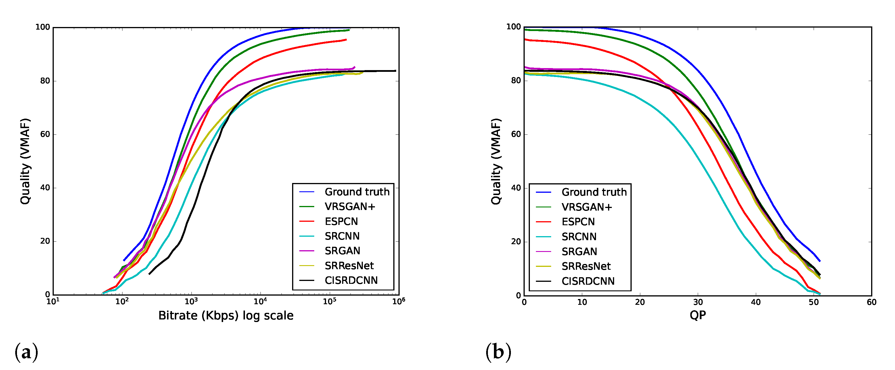
Second, we applied VMAF to evaluate the perceptual quality of the videos by changing the bitrate through QP in $[0;51]$. We compare the quality of two-fold upscaled videos, i.e., 540p to 1080p, using VSRGAN+ and the other models in Table 1. We also compare them with compressed videos within the range of 0 to 51 alone.

Figure 4 presents the assessed perceptual quality. In Figure 4a, the quality considers the compression levels in bitrates; Figure 4b includes the compression levels according to the QP. The results show that the VSRGAN+ model outperformed the quality presented by the other models for compression levels up to 42 QP; only for compression levels greater than 42 QP did the CISRDCNN model outperform VSRGAN+.

The training of models uses images of the Places365-Standard dataset [60], except for the model CISRDCNN, which uses images with compression artifacts, defined by the quality factor (QF) 20 JPEG, applied for the same dataset. Although the CISRDCNN model targets images with compression artifacts, it did not stand out in our experiments even when we used compressed videos. We assess the quality using the VMAF, a perceptual metric, and the training of CISRDCNN works to optimize the pixel-wise quality. However, pixel-wise metrics, such as PSNR, struggle to express human visual perception [21,33,58].

The general conclusion is that the VSRGAN+ model showed the best outcomes among the three metrics: VMAF, PSNR, and LPIPS. The model’s loss function (Equation (4)) considers pixel-wise and perceptual-wise features. This shows the versatility of the proposed model by learning how to score high values concerning those metrics.

The VSRGAN+ model showed the highest results regarding perceptual quality among the evaluated SR models. We used state-of-the-art SISR [22] building blocks, namely: (i) GAN with a relativistic discriminator; (ii) residual-in-residual dense blocks; (iii) skip connections; (iv) enhanced perceptual loss function, and (v) upsampling with the subpixel layer. Adversarial training with a perceptual loss function contributes to a model capable of super-resolving videos with sharp images that are perceptually indistinguishable from the ground truth.

7.3. Perceptual Quality and JND

This subsection analyzes how the perceptual and pixel-wise metrics perceive video compression distortions. First, we examine the JND mapping, using the QP to obtain the desired video bitrates. Then, for the same set of video bitrates, we examine the PSNR mapping. Wang et al. [48] presented JND mapping of the analyzed video sequences.

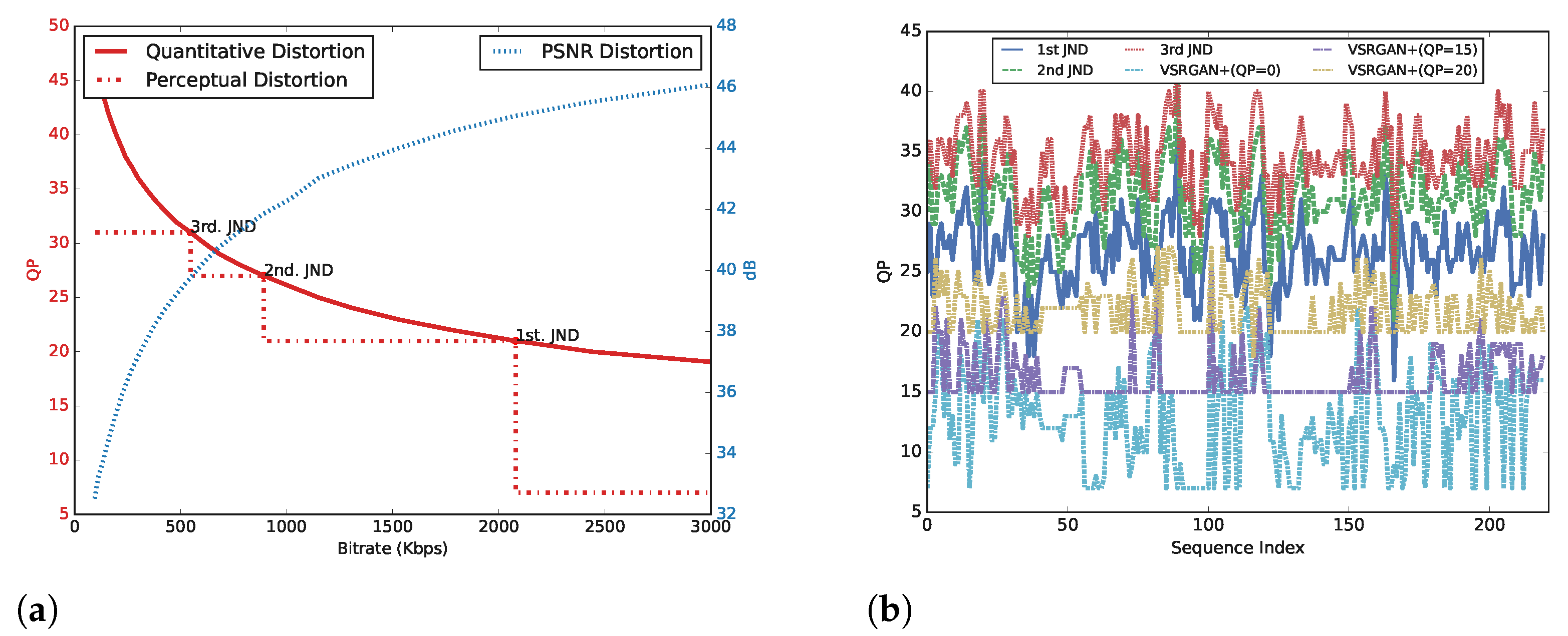
Figure 5a shows the outcomes for a 1080p video sequence, #112 of the VideoSet dataset. This video sequence was encoded using a broad range of bitrates from 94 kbps ($QP=47$) to $264,088$ kbps $(QP=7)$. From a pixel-wise point of view, the general conclusion was that the encoding bitrate increases quickly as the quantization parameter decreases. A small QP indicates that the encoding process uses a low compression rate. Moreover, PSNR mapping can capture the changes in the encoding bitrate as it transitions from low to high values.

From a perceptual point of view, the JND mapping identified three distortion points, i.e., $QP=\{21,27,31\}$, perceived by the human vision system. In other words, QP values taken from the encoding spectrum $[0,21[$ will result in encoding distortions unnoticed by the human visual system. Similar conclusions were derived for other encoding spectra: $QP=\left\{\right[21,27[,[27,31[,[31,51\left]\right\}$. These values are closely related to the analyzed video sequence. Still, the general conclusion is that human vision cannot perceive visual quality improvements among encoded videos in the same encoding spectrum.

The super-resolved video sequences ($V^{SR}$) were analyzed to determine their closest ground-truth encoded versions ($V^{HD}$) and map the reconstructed video sequence to the JND encoding spectrum associated with the ground-truth video sequence. Equation (10) calculates the distance between the reconstructed video sequence and all encoded video sequences.

$$Q{P}_{V_{i,k}^{SR}}=j,\mathrm{where}j=min\left(D\left(V_{i,k}^{SR},V_{i,j}^{HR}\right)\right)$$

(10)

D is the perceptual distance LPIPS; $k=\{0,15,20\}$ is the QP used to encode the video sequence that was in the restoration, among $i=\{1,\dots ,220\}$ possibilities; $j=\{7,\dots ,47\}$ is the QP of encoded video sequences $V^{HR}$; $V_{i,k}^{SR}$ is given by

$$V_{i,k}^{SR}\in \left\{\begin{array}{cc}& Q_1,\mathrm{if}Q{P}_{V_{i,k}^{SR}}<Q{P}_{1^{st}JND,i}\hfill \\ & Q_2,\mathrm{if}Q{P}_{1^{st}JND,i}\le Q{P}_{V_{i,k}^{SR}}<Q{P}_{2^{nd}JND,i}\hfill \\ & Q_3,\mathrm{if}Q{P}_{2^{nd}JND,i}\le Q{P}_{V_{i,k}^{SR}}<Q{P}_{3^{rd}JND,i}\hfill \\ & Q_4,\mathrm{if}Q{P}_{V_{i,k}^{SR}}\ge Q{P}_{3^{rd}JND,i},\hfill \end{array}\right.$$

where $Q{P}_{1^{st}JND,i},Q{P}_{2^{nd}JND,i}$, and $Q{P}_{3^{nd}JND,i}$$\in Q{P}_{V_i^{HR}}$.

Figure 5b shows all 1080p video sequences from the VideoSet dataset, with JND points calculated using Equation (10). We calculated these points for video sequences encoded using $QP=\{0,15,20\}$ and those super-resolved by the VSRGAN+ model. When the ground-truth video sequences were encoded using $QP=\{0,15\}$, the evaluation showed that 100% of the super-resolved video sequences were within the set $Q_1$. The ground-truth video sequences, encoded with $QP=20$, included $91.4\%$ of the super-resolved video sequences in $Q_1$ and $8.6\%$ in $Q_2$. In summary, the super-resolved video sequences had a perceptual quality similar to their ground-truth counterparts.

7.4. Runtime Analysis

Figure 6 shows the average run time of experiments that super-resolved video sequences that lasted one second and were encoded in high definition, i.e., 720p and 1080p. The quality of these super-resolved sequences was assessed by the VMAF metric. The proposed model, i.e., VSRGAN+, had a middle-ground computational cost. It was higher than the cost of the SRCNN and ESPCN models but lower than that of the SRResNet and SRGAN models. This middle-ground performance paid off by enabling the VSRGAN+ to achieve the highest perceptual quality assessed by the VMAF metric.

The proposed video distribution architecture supports VoD applications; see Section 3. In this scenario, any publisher committed to high-standards of perceptual quality would agree to postpone the content release time to have the best output for the publishing step. This reasoning reinforces the importance of balancing the computational cost and the perceptual quality of super-resolved video clips, which is the case of the VSRGAN+ model.

7.5. Data Transfer Decrease

This subsection presents the evaluation to measure the decrease in the amount of data that flows throughout the networking infrastructure. This infrastructure connects the video source and surrogate servers that distribute video sequences in mono-resolution and multi-resolution modalities.

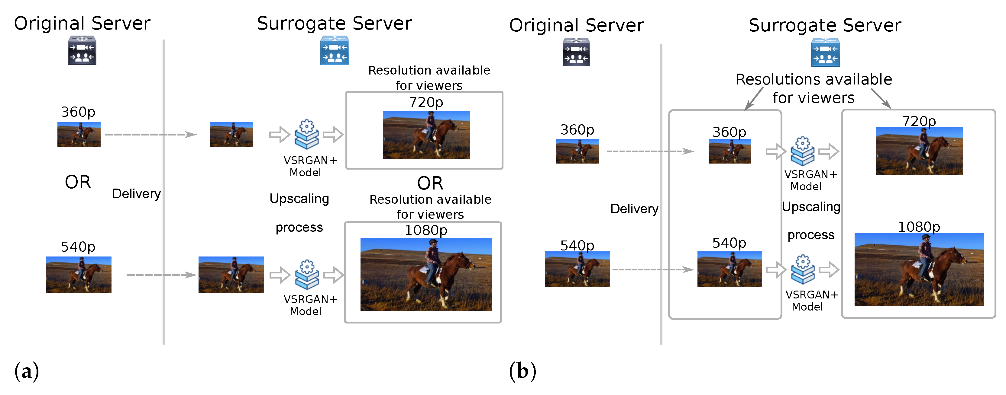
In the first scenario, we show the decrease in data transfer for a mono-resolution modality. In this modality, the assumption is that low-resolution videos $V^{LR}$ encoded in 360p or 540p are super-resolved using a 2× factor, and engaged audiences access this content at 720p or 1080p resolution (see Figure 7a).

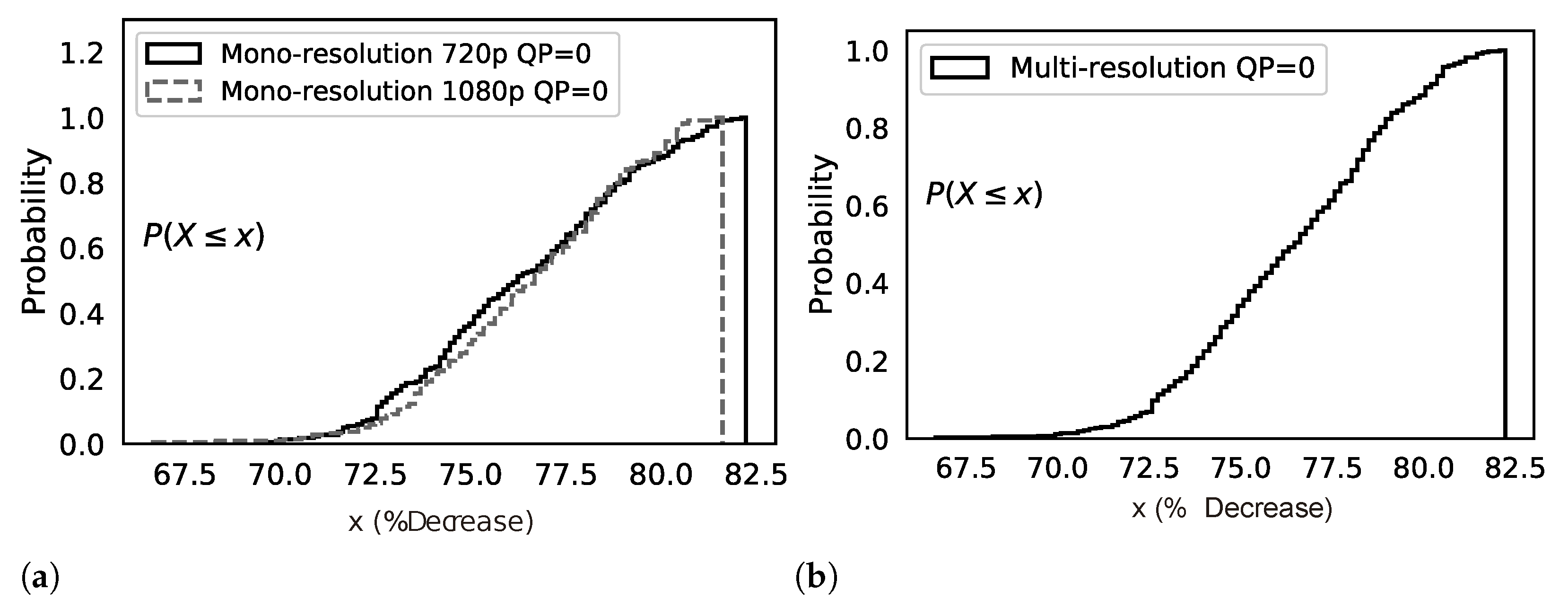
Figure 8a shows the CDF of the decrease in data transfer for the mono-resolution modality. The low-resolution streams, i.e., 360p and 540p, have the highest quality ($QP=0$), and we used 220 video sequences. Equation (11) gives the decrease in the amount of data.

$$D_{ecreasing}\left(V_i\right)=1-\frac{size\left(V_i^{LR}\right)}{size\left(V_i^{HR}\right)}$$

(11)

In the 360p mono-resolution modality, the probability is zero that the decrease in data transfer will reach a value less than $69.48\%$, and the probability is $100\%$ that the decrease in data transfer will reach $82.23\%$. In other words, this decrease will be in the range of $69.48\%$ and $82.23\%$. The decrease in the 540p mono-resolution modality will be from $66.67\%$ to $81.61\%$.

Numerically, the 360p mono-resolution modality has 220 video sequences that demand 13.64 GB on data transfer, i.e., 2.6 GB (360p) and 11.04 GB (760 p), a decrease equal to $76.45\%$ results in less than 8.44 GB going into the video service infrastructure. The 560p mono-resolution modality has 220 video sequences, the demands on data transfer are 6.0 GB (540p) and 25.9 GB (1080p), and a decrease equal to $76.8\%$ results in less 19.9 GB going into that infrastructure.

Figure 8b shows the CDF of the multi-resolution modality, i.e., we transmit 360p and 540p video sequences to surrogate servers and super-resolved them to 720p and 1080p, respectively. In this scenario, four versions of each video sequence are available to audiences as shown in Figure 7b.

Equation (12) gives the decrease in data transfer.

$$\begin{array}{c}\hfill D_{ecreasing}\left(V_i\right)=1-\frac{size\left(V_i{}_{360p}^{LR}+V_i{}_{540p}^{LR}\right)}{size\left(V_i{}_{360p}^{LR}+V_i{}_{540p}^{LR}+V_i{}_{720p}^{HR}+V_i{}_{1080p}^{HR}\right)}\end{array}$$

(12)

Figure 8b shows the CDF of the decrease in data transfer for the multi-resolution modality. The decrease ranges from $75.67\%$ to $84.59\%$. Numerically, 8.63 GB is the amount of data demanded by low-resolution videos (360p and 540p). In contrast, 45.57 GB is the amount of data after the super-resolving procedure, which includes the four resolutions, i.e., 360p, 540p, 720p, and 1080p, resulting in an absolute gain of 36.94 GB. This results in $81.06\%$ fewer data going into the distribution infrastructure to serve the audience from the surrogate servers.

7.6. Data Reduction Using Super-Resolution vs. Compression

We analyzed the reduction in data when super-resolution was used and compared it with data reduction when applying compression. The general approach uses levels of compression, i.e., changing the QP, during the video encoding step to reduce the amount of data.

The study in Section 7.3 sheds light on how we can combine super-resolution with compression without affecting the perceptual quality of videos. In this regard, we also analyzed the data transfer decrease when we combined those two approaches.

Table 5. The average size of videos with $QP=\{0,10,15,20,25\}$ variations.

QP	360p	540p	720p	1080p
0	11.80 Mb $(\pm 0.54)$	27.43 Mb $(\pm 1.20)$	50.18 Mb $(\pm 2.16)$	117.71 Mb $(\pm 5.07)$
10	4.74 Mb $(\pm 0.44)$	11.20 Mb $(\pm 0.97)$	21.42 Mb $(\pm 1.75)$	53.76 Mb $(\pm 4.13)$
15	2.38 Mb $(\pm 0.29)$	5.01 Mb $(\pm 0.62)$	9.00 Mb $(\pm 1.09)$	22.81 Mb $(\pm 2.54)$
20	1.24 Mb $(\pm 0.18)$	2.35 Mb $(\pm 0.35)$	3.80 Mb $(\pm 0.58)$	8.18 Mb $(\pm 1.28)$
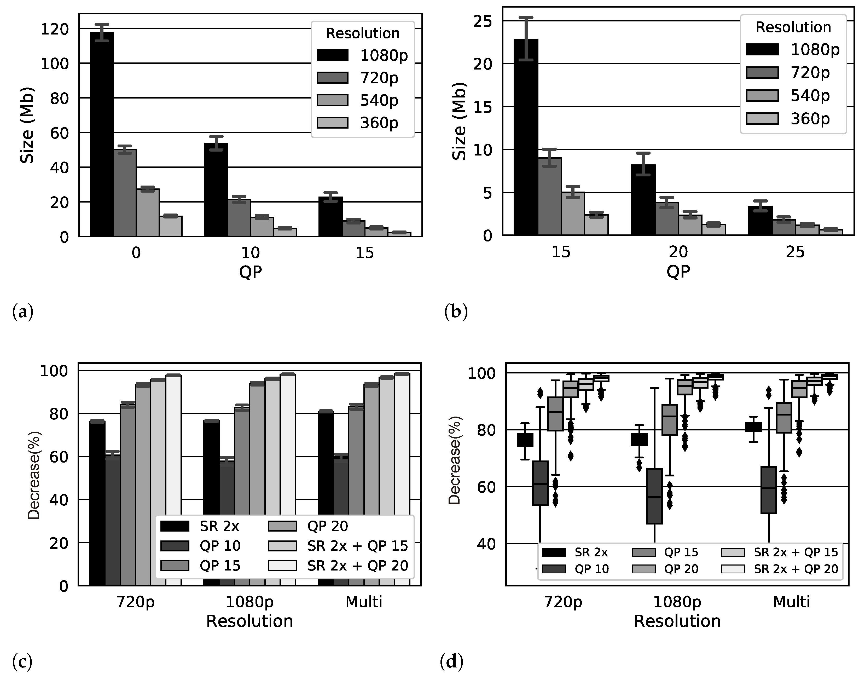
25	0.65 Mb $(\pm 0.10)$	1.18 Mb $(\pm 0.20)$	1.80 Mb $(\pm 0.32)$	3.38 Mb $(\pm 0.59)$

shows the average sizes with a 95% confidence interval of the 220 video samples at resolutions of 360p, 540p, 720p, and 1080p and presents the variation in compression levels as a function of $QP=\{0,10,15,20,25\}$.

Figure 9a,b show exponential decay in the average size of the videos as we reduce the resolution and compression in QP levels. It suggests that reducing the volume of data transmitted by applying compression and reducing resolution is possible. To prove this, we analyzed the decrease in the amount of data transmitted using videos with QP = 0 as the baseline.

Table 6. Decrease over mono-resolution and multi-resolution delivery and compression level.

Data Reduction	Mono-Resolution 720p	Mono-Resolution 1080p	Multi Resolution
SR 2×	76.35% $(\pm 0.38)$	76.52% $(\pm 0.35)$	80.99% $(\pm 0.23)$
QP10	60.67% $(\pm 1.73)$	57.83% $(\pm 1.78)$	59.28% $(\pm 1.69)$
QP15	84.13% $(\pm 1.23)$	82.80% $(\pm 1.22)$	83.12% $(\pm 1.18)$
QP20	93.34% $(\pm 0.69)$	93.91% $(\pm 0.65)$	93.37% $(\pm 0.68)$
SR 2×+QP15	95.62% $(\pm 0.36)$	96.07% $(\pm 0.34)$	96.74% $(\pm 0.27)$
SR 2×+QP20	97.74% $(\pm 0.22)$	98.14% $(\pm 0.20)$	98.42% $(\pm 0.16)$

shows the decrease for the mono-resolution (720p and 1080p) and multi-resolution modalities as shown in Figure 7. All the points are average values with a 95% confidence interval.

Figure 9c shows the decrease in data transfer. The super-resolution decrease in 2× (SR 2×) is better than the compression decrease with $QP=10$ in mono-resolution and multi-resolution. The combination of SR 2× with $QP=15$ decreased more than $QP=15$ or $QP=20$, and the highest decrease happened when combining SR 2× + QP 20. This achieved 97.4%, 98.14%, and 98.42% for 720p, 1080p, and multi-resolution and mono-resolution modalities, respectively.

We also analyzed the amplitude of the decrease in the 220 samples as illustrated in the boxplot in Figure 9d. The decreases from compression were more dispersed than the decreases from SR, which, in Table 6, showed larger confidence intervals for compression. Such dispersion occurs more in compression because it is intrinsically related to how the compression exploits the pixels and frames of the videos, i.e., the compression may be higher or lower depending on the correlation of frames. In the SR, the decrease is more uniform since there is a reduction in the resolution size; therefore, it presents less dispersion in decreases, bolded by smaller amplitudes of the SR boxplots in Figure 9d.

8. Conclusions

In a cloud-based video streaming framework, we super-resolved low-resolution videos using the VSRGAN+ neural network model to reduce the costs associated with the data traffic between the original server and the surrogate servers. We upscaled videos using the VSRGAN+ model, a deep neural network with a perceptual-driven loss function and tailored layers fitting the limited computing resources of the surrogate servers. We showed that the proposed framework promoted a decrease in data traffic of up to 98.42%, when comparing the SR-based content placement approach and a lossless compression-based one.

To assess the quality of the super-resolved videos, we considered these three metrics: LPIPS, VMAF, and PSNR. We showed that super-revolved videos obtained by a 2x-factor training VSRGAN+ model preserved the perceptual quality, i.e., the super-resolved videos were indistinguishable from the original videos.

The future direction of this research looks at edge-computing paradigms to explore computing resources on edge servers and end-user devices to support real-time SR. This could improve the quality of video sessions under severe restrictions on throughput on both fronthaul and backhaul networks.

References

1. Cisco VNI. Cisco Visual Networking Index: Forecast and Trends, 2017–2022 White Paper; Technical Report; Cisco. 2019. Available online: https://twiki.cern.ch/twiki/pub/HEPIX/TechwatchNetwork/HtwNetworkDocuments/white-paper-c11-741490.pdf (accessed on 5 September 2022).
2. Zolfaghari, B.; Srivastava, G.; Roy, S.; Nemati, H.R.; Afghah, F.; Koshiba, T.; Razi, A.; Bibak, K.; Mitra, P.; Rai, B.K. Content Delivery Networks: State of the Art, Trends, and Future Roadmap. ACM Comput. Surv. 2020, 53, 34. [Google Scholar] [CrossRef]
3. Li, Z.; Wu, Q.; Salamatian, K.; Xie, G. Video Delivery Performance of a Large-Scale VoD System and the Implications on Content Delivery. IEEE Trans. Multimed. 2015, 17, 880–892. [Google Scholar] [CrossRef]
4. BITMOVIN INC. Per-Title Encoding. 2020. Available online: https://bitmovin.com/demos/per-title-encoding (accessed on 5 September 2022).
5. Yan, B.; Shi, S.; Liu, Y.; Yuan, W.; He, H.; Jana, R.; Xu, Y.; Chao, H.J. LiveJack: Integrating CDNs and Edge Clouds for Live Content Broadcasting. In Proceedings of the 25th ACM International Conference on Multimedia, Mountain View, CA, USA, 23–27 October 2017; Association for Computing Machinery: New York, NY, USA, 2017; pp. 73–81. [Google Scholar] [CrossRef]
6. Yeo, H.; Jung, Y.; Kim, J.; Shin, J.; Han, D. Neural Adaptive Content-aware Internet Video Delivery. In Proceedings of the 13th USENIX Symposium on Operating Systems Design and Implementation (OSDI 18), Carlsbad, CA, USA, 8–10 October 2018; USENIX Association: Berkeley, CA, USA, 2018; pp. 645–661. [Google Scholar]
7. Wang, F.; Zhang, C.; Wang, F.; Liu, J.; Zhu, Y.; Pang, H.; Sun, L. DeepCast: Towards Personalized QoE for Edge-Assisted Crowdcast With Deep Reinforcement Learning. IEEE/ACM Trans. Netw. 2020, 28, 1255–1268. [Google Scholar] [CrossRef]
8. Liborio, J.M.; Souza, C.M.; Melo, C.A.V. Super-resolution on Edge Computing for Improved Adaptive HTTP Live Streaming Delivery. In Proceedings of the 2021 IEEE tenth International Conference on Cloud Networking (CloudNet), Cookeville, TN, USA, 8–10 November 2021; pp. 104–110. [Google Scholar] [CrossRef]
9. Yeo, H.; Do, S.; Han, D. How Will Deep Learning Change Internet Video Delivery? In Proceedings of the 16th ACM Workshop on Hot Topics in Networks, Palo Alto, CA, USA, 30 November–1 December 2017; ACM: New York, NY, USA, 2017; pp. 57–64. [Google Scholar] [CrossRef]
10. Hecht, J. The bandwidth bottleneck that is throttling the Internet. Nature 2016, 536, 139–142. [Google Scholar] [CrossRef] [PubMed] [Green Version]
11. Christian, P. Int’l Bandwidth and Pricing Trends; Technical Report; TeleGeography: 2018. Available online: https://www.afpif.org/wp-content/uploads/2018/08/01-International-Internet-Bandwidth-and-Pricing-Trends-in-Africa-%E2%80%93-Patrick-Christian-Telegeography.pdf (accessed on 5 September 2022).
12. Wang, Z.; Sun, L.; Wu, C.; Zhu, W.; Yang, S. Joint online transcoding and geo-distributed delivery for dynamic adaptive streaming. In Proceedings of the IEEE INFOCOM 2014—IEEE Conference on Computer Communications, Toronto, ON, Canada, 27 April–2 May 2014; pp. 91–99. [Google Scholar] [CrossRef] [Green Version]
13. AI IMPACTS. 2019 recent trends in GPU price per FLOPS. Technical report, AI IMPACTS. 2019. Available online: https://aiimpacts.org/2019-recent-trends-in-gpu-price-per-flops (accessed on 16 August 2022).
14. NVIDIA Corporation. Accelerated Computing Furthermore, The Democratization Of Supercomputing; Technical Report; California, USA, NVIDIA Corporation: 2018. Available online: https://www.nvidia.com/content/dam/en-zz/Solutions/Data-Center/tesla-product-literature/sc18-tesla-democratization-tech-overview-r4-web.pdf (accessed on 16 August 2022).
15. Cloud, G. Cheaper Cloud AI Deployments with NVIDIA T4 GPU Price Cut; Technical Report; California, USA, Google: 2020. Available online: https://cloud.google.com/blog/products/ai-machine-learning/cheaper-cloud-ai-deployments-with-nvidia-t4-gpu-price-cut (accessed on 16 August 2022).
16. Papidas, A.G.; Polyzos, G.C. Self-Organizing Networks for 5G and Beyond: A View from the Top. Future Internet 2022, 14, 95. [Google Scholar] [CrossRef]
17. Dong, J.; Qian, Q. A Density-Based Random Forest for Imbalanced Data Classification. Future Internet 2022, 14, 90. [Google Scholar] [CrossRef]
18. Kappeler, A.; Yoo, S.; Dai, Q.; Katsaggelos, A.K. Video Super-Resolution With Convolutional Neural Networks. IEEE Trans. Comput. Imaging 2016, 2, 109–122. [Google Scholar] [CrossRef]
19. Pérez-Pellitero, E.; Sajjadi, M.S.M.; Hirsch, M.; Schölkopf, B. Photorealistic Video Super Resolution. arXiv 2018, arXiv:1807.07930. [Google Scholar]
20. Karras, T.; Aila, T.; Laine, S.; Lehtinen, J. Progressive Growing of GANs for Improved Quality, Stability, and Variation. arXiv 2018, arXiv:1710.10196. [Google Scholar]
21. Ledig, C.; Theis, L.; Huszar, F.; Caballero, J.; Aitken, A.P.; Tejani, A.; Totz, J.; Wang, Z.; Shi, W. Photo-Realistic Single Image Super-Resolution Using a Generative Adversarial Network. arXiv 2018, arXiv:1609.04802. [Google Scholar]
22. Wang, X.; Yu, K.; Wu, S.; Gu, J.; Liu, Y.; Dong, C.; Qiao, Y.; Loy, C.C. ESRGAN: Enhanced super-resolution generative adversarial networks. In Computer Vision—ECCV 2018 Workshops; Leal-Taixé, L., Roth, S., Eds.; Springer International Publishing: Cham, Switzerland, 2019; pp. 63–79. [Google Scholar]
23. Lucas, A.; Tapia, S.L.; Molina, R.; Katsaggelos, A.K. Generative Adversarial Networks and Perceptual Losses for Video Super-Resolution. arXiv 2018, arXiv:1806.05764. [Google Scholar]
24. He, Z.; Cao, Y.; Du, L.; Xu, B.; Yang, J.; Cao, Y.; Tang, S.; Zhuang, Y. MRFN: Multi-Receptive-Field Network for Fast and Accurate Single Image Super-Resolution. IEEE Trans. Multimed. 2020, 22, 1042–1054. [Google Scholar] [CrossRef]
25. Wang, J.; Teng, G.; An, P. Video Super-Resolution Based on Generative Adversarial Network and Edge Enhancement. Electronics 2021, 10, 459. [Google Scholar] [CrossRef]
26. Yang, W.; Zhang, X.; Tian, Y.; Wang, W.; Xue, J.; Liao, Q. Deep Learning for Single Image Super-Resolution: A Brief Review. IEEE Trans. Multimed. 2019, 21, 3106–3121. [Google Scholar] [CrossRef] [Green Version]
27. Anwar, S.; Khan, S.; Barnes, N. A Deep Journey into Super-Resolution: A Survey. ACM Comput. Surv. 2020, 53, 60. [Google Scholar] [CrossRef]
28. Dong, C.; Loy, C.C.; He, K.; Tang, X. Learning a Deep Convolutional Network for Image Super-Resolution. In Computer Vision—ECCV 2014; Fleet, D., Pajdla, T., Schiele, B., Tuytelaars, T., Eds.; Springer International Publishing: Cham, Switzerland, 2014; pp. 184–199. [Google Scholar]
29. Dong, C.; Loy, C.C.; He, K.; Tang, X. Image Super-Resolution Using Deep Convolutional Networks. IEEE Trans. Pattern Anal. Mach. Intell. 2016, 38, 295–307. [Google Scholar] [CrossRef] [Green Version]
30. Dong, C.; Loy, C.C.; Tang, X. Accelerating the Super-Resolution Convolutional Neural Network. arXiv 2016, arXiv:1608.00367. [Google Scholar]
31. Chen, H.; He, X.; Ren, C.; Qing, L.; Teng, Q. CISRDCNN: Super-resolution of compressed images using deep convolutional neural networks. Neurocomputing 2018, 285, 204–219. [Google Scholar] [CrossRef] [Green Version]
32. Shi, W.; Caballero, J.; Huszár, F.; Totz, J.; Aitken, A.P.; Bishop, R.; Rueckert, D.; Wang, Z. Real-Time Single Image and Video Super-Resolution Using an Efficient Sub-Pixel Convolutional Neural Network. arXiv 2016, arXiv:1609.05158. [Google Scholar]
33. Johnson, J.; Alahi, A.; Li, F. Perceptual Losses for Real-Time Style Transfer and Super-Resolution. arXiv 2016, arXiv:1603.08155. [Google Scholar]
34. Haris, M.; Shakhnarovich, G.; Ukita, N. Recurrent Back-Projection Network for Video Super-Resolution. arXiv 2019, arXiv:1903.10128. [Google Scholar]
35. Tian, Y.; Zhang, Y.; Fu, Y.; Xu, C. TDAN: Temporally Deformable Alignment Network for Video Super-Resolution. arXiv 2018, arXiv:1812.02898. [Google Scholar]
36. Wang, X.; Chan, K.C.K.; Yu, K.; Dong, C.; Loy, C.C. EDVR: Video Restoration with Enhanced Deformable Convolutional Networks. arXiv 2019, arXiv:1905.02716. [Google Scholar]
37. Jo, Y.; Oh, S.W.; Kang, J.; Kim, S.J. Deep Video Super-Resolution Network Using Dynamic Upsampling Filters Without Explicit Motion Compensation. In Proceedings of the IEEE Conference on Computer Vision and Pattern Recognition (CVPR), Salt Lake City, UT, USA, 18–23 June 2018. [Google Scholar]
38. Isobe, T.; Zhu, F.; Jia, X.; Wang, S. Revisiting Temporal Modeling for Video Super-resolution. arXiv 2020, arXiv:2008.05765. [Google Scholar]
39. Chadha, A.; Britto, J.; Roja, M.M. iSeeBetter: Spatio-temporal video super-resolution using recurrent generative back-projection networks. Comput. Vis. Media 2020, 6, 307–317. [Google Scholar] [CrossRef]
40. Nah, S.; Baik, S.; Hong, S.; Moon, G.; Son, S.; Timofte, R.; Lee, K.M. NTIRE 2019 Challenge on Video Deblurring and Super-Resolution: Dataset and Study. In Proceedings of the 2019 IEEE/CVF Conference on Computer Vision and Pattern Recognition Workshops (CVPRW), Long Beach, CA, USA, 16–17 June 2019; pp. 1996–2005. [Google Scholar]
41. Liu, C.; Sun, D. A Bayesian approach to adaptive video super resolution. In Proceedings of the CVPR 2011, Washington, DC, USA, 20–25 June 2011; pp. 209–216. [Google Scholar]
42. Xue, T.; Chen, B.; Wu, J.; Wei, D.; Freeman, W.T. Video Enhancement with Task-Oriented Flow. arXiv 2017, arXiv:1711.09078. [Google Scholar] [CrossRef] [Green Version]
43. Tao, X.; Gao, H.; Liao, R.; Wang, J.; Jia, J. Detail-Revealing Deep Video Super-Resolution. In Proceedings of the 2017 IEEE International Conference on Computer Vision (ICCV), Venice, Italy, 22–29 October 2017; pp. 4482–4490. [Google Scholar]
44. Liborio, J.M.; Melo, C.A.V. A GAN to Fight Video-related Traffic Flooding: Super-resolution. In Proceedings of the 2019 IEEE Latin-American Conference on Communications (LATINCOM), Salvador, Brazil, 11–13 November 2019; pp. 1–6. [Google Scholar] [CrossRef]
45. Lubin, J. A human vision system model for objective image fidelity and target detectability measurements. In Proceedings of the Ninth European Signal Processing Conference (EUSIPCO 1998), Rhodes, Greece, 8–11 September 1998; pp. 1–4. [Google Scholar]
46. Watson, A.B. Proposal: Measurement of a JND scale for video quality. IEEE G-2.1. 6 Subcommittee on Video Compression Measurements; Citeseer. 2000. Available online: https://citeseerx.ist.psu.edu/document?repid=rep1&type=pdf&doi=2c57d52b6fcdd4e967f9a39e6e7509d948e57a07 (accessed on 21 July 2021).
47. Lin, J.Y.c.; Jin, L.; Hu, S.; Katsavounidis, I.; Li, Z.; Aaron, A.; Kuo, C.C.J. Experimental design and analysis of JND test on coded image/video. In Proceedings of the Applications of Digital Image Processing XXXVIII, San Diego, CA, USA, 10–13 August 2015; p. 95990Z. [Google Scholar] [CrossRef]
48. Wang, H.; Katsavounidis, I.; Zhou, J.; Park, J.; Lei, S.; Zhou, X.; Pun, M.; Jin, X.; Wang, R.; Wang, X.; et al. VideoSet: A Large-Scale Compressed Video Quality Dataset Based on JND Measurement. arXiv 2017, arXiv:1701.01500. [Google Scholar] [CrossRef]
49. Zhang, R.; Isola, P.; Efros, A.A.; Shechtman, E.; Wang, O. The Unreasonable Effectiveness of Deep Features as a Perceptual Metric. arXiv 2018, arXiv:1801.03924. [Google Scholar]
50. Huang, C.; Wang, A.; Li, J.; Ross, K.W. Measuring and evaluating large-scale CDNs. In Proceedings of the ACM IMC, Vouliagmeni, Greece, 20–22 October 2008. [Google Scholar]
51. Goodfellow, I.J.; Pouget-Abadie, J.; Mirza, M.; Xu, B.; Warde-Farley, D.; Ozair, S.; Courville, A.; Bengio, Y. Generative Adversarial Networks. arXiv 2014, arXiv:1406.2661. [Google Scholar] [CrossRef]
52. He, K.; Zhang, X.; Ren, S.; Sun, J. Delving Deep into Rectifiers: Surpassing Human-Level Performance on ImageNet Classification. arXiv 2015, arXiv:11502.01852. [Google Scholar]
53. Maas, A.L. Rectifier Nonlinearities Improve Neural Network Acoustic Models. In Proceedings of the ICML, Atlanta, GA, USA, 16–21 June 2013. [Google Scholar]
54. Szegedy, C.; Ioffe, S.; Vanhoucke, V. Inception-v4, Inception-ResNet and the Impact of Residual Connections on Learning. arXiv 2016, arXiv:1602.07261. [Google Scholar] [CrossRef]
55. Jolicoeur-Martineau, A. The relativistic discriminator: A key element missing from standard GAN. arXiv 2018, arXiv:1807.00734. [Google Scholar]
56. Zhao, H.; Gallo, O.; Frosio, I.; Kautz, J. Loss Functions for Image Restoration With Neural Networks. IEEE Trans. Comput. Imaging 2017, 3, 47–57. [Google Scholar] [CrossRef]
57. Mathieu, M.; Couprie, C.; LeCun, Y. Deep multi-scale video prediction beyond mean square error. arXiv 2015, arXiv:1511.05440. [Google Scholar]
58. Bruna, J.; Sprechmann, P.; LeCun, Y. Super-Resolution with Deep Convolutional Sufficient Statistics. arXiv 2015, arXiv:1511.05666. [Google Scholar]
59. Simonyan, K.; Zisserman, A. Very Deep Convolutional Networks for Large-Scale Image Recognition. arXiv 2014, arXiv:1409.1556. [Google Scholar]
60. Zhou, B.; Lapedriza, A.; Khosla, A.; Oliva, A.; Torralba, A. Places: A 10 million Image Database for Scene Recognition. IEEE Trans. Pattern Anal. Mach. Intell. 2017. [Google Scholar] [CrossRef] [Green Version]
61. Zhang, K.; Gu, S.; Timofte, R. NTIRE 2020 Challenge on Perceptual Extreme Super-Resolution: Methods and Results. In Proceedings of the 2020 IEEE/CVF Conference on Computer Vision and Pattern Recognition Workshops (CVPRW), Seattle, WA, USA, 14–19 June 2020; pp. 2045–2057. [Google Scholar] [CrossRef]
62. Iandola, F.N.; Moskewicz, M.W.; Ashraf, K.; Han, S.; Dally, W.J.; Keutzer, K. SqueezeNet: AlexNet-level accuracy with 50x fewer parameters and <1MB model size. arXiv 2016, arXiv:1602.07360. [Google Scholar]
63. Krizhevsky, A.; Sutskever, I.; Hinton, G.E. ImageNet Classification with Deep Convolutional Neural Networks. In Proceedings of the 25th International Conference on Neural Information Processing Systems, New York, NY, USA, 3–6 December; Curran Associates Inc.: New York, NY, USA, 2012; Volume 1, pp. 1097–1105. [Google Scholar]
64. Li, Z.; Bampis, C.; Novak, J.; Aaron, A.; Swanson, K.; Moorthy, A.; Cock, J.D. VMAF: The Journey Continues. Online, Netflix Technology Blog. 2018. Available online: https://netflixtechblog.com/vmaf-the-journey-continues-44b51ee9ed12 (accessed on 15 July 2021).
65. Aaron, A.; Li, Z.; Manohara, M.; Lin, J.Y.; Wu, E.C.H.; Kuo, C.C.J. Challenges in cloud based ingest and encoding for high quality streaming media. In Proceedings of the 2015 IEEE International Conference on Image Processing (ICIP), Quebec City, QC, Canada, 27–30 September 2015; pp. 1732–1736. [Google Scholar] [CrossRef]
Figure 1. The content-placement framework of cloud-based video-streaming services.
Futureinternet 14 00364 g001
Figure 2. The generator architecture and relativistic average discriminator networks: (1) Pre-residual blocks in the generator; (2) Residual in residual blocks in the generator; (3) Upscaling blocks in the generator; (4) Discriminator blocks; and (5) The relativistic average discriminator component.
Futureinternet 14 00364 g002
Figure 3. Restoration video quality assessment using PSNR, LPIPS, and VMAF. (a) The PSNR quality assessment. (b) The LPIPS quality assessment. (c) The VMAF quality assessment.
Futureinternet 14 00364 g003
Figure 4. Perceptual quality assessment of videos 2× upscaled by SR methods given videos with different bitrates. (a) VMAF scores for videos encoded at different bitrates. (b) VMAF scores for videos encoded with different quantization parameters.
Futureinternet 14 00364 g004
Figure 5. Visual perception analysis of V S R super-resolved videos. (a) Comparing JND and PSNR sensitivity to video distortion. (b) Comparing V S R encoded with Q P = 0 , 15 , 20 and the JND points 1st, 2nd, and 3rd.
Futureinternet 14 00364 g005
Figure 6. The average running time versus the VMAF assessed video quality. (a) Video sequence with 720p. (b) Video sequence with 1080p.
Futureinternet 14 00364 g006
Figure 7. The super-resolution-based content distribution policy for mono- and multi-resolution services. (a) Monoresolution service: 720p or 1080p resolution. (b) Multiresolution service: 360p, 540p, 720p, and 1080p.
Futureinternet 14 00364 g007
Figure 8. CDFs of the gain in data volume: 2× factor SR in mono-resolution and multi-resolution modalities. (a) CDFs of the gain in a mono-resolution. (b) CDFs of the gain in a multi-resolution adaptive stream.
Futureinternet 14 00364 g008
Figure 9. The average size of videos encoded in different resolutions and levels of compression and the decrease in networking traffic for mono-resolution and multi-resolution modalities. (a) Average video size in Mb with variation Q P = { 0 , 10 , 15 } . (b) Average video size in Mb with variation Q P = { 15 , 20 , 25 } . (c) Decrease in mono-resolution and multi-resolution distribution with SR and compression. (d) Boxplot of gains in mono-resolution and multi-resolution distribution.
Futureinternet 14 00364 g009