Article

Topology Inference and Link Parameter Estimation Based on End-to-End Measurements †

by
Grigorios Kakkavas
1,
Vasileios Karyotis
1,2 and
Symeon Papavassiliou
1,*
1
School of Electrical and Computer Engineering, National Technical University of Athens, Iroon Polytechniou 9, 15780 Athens, Greece
2
Department of Informatics, Ionian University, 49100 Corfu, Greece
*
Author to whom correspondence should be addressed.
This paper is an extended version of our paper published in the Proceedings of ICC 2020—2020 IEEE International Conference on Communications (ICC), A Distance-Based Agglomerative Clustering Algorithm for Multicast Network Tomography, Dublin, Ireland, 7–11 June 2020.
Future Internet 2022, 14(2), 45; https://doi.org/10.3390/fi14020045
Submission received: 8 January 2022 / Revised: 26 January 2022 / Accepted: 27 January 2022 / Published: 28 January 2022
(This article belongs to the Special Issue Modern Trends in Multi-Agent Systems)

Abstract

:
This paper focuses on the design, implementation, experimental validation, and evaluation of a network tomography approach for performing inferential monitoring based on indirect measurements. In particular, we address the problems of inferring the routing tree topology (both logical and physical) and estimating the links’ loss rate and jitter based on multicast end-to-end measurements from a source node to a set of destination nodes using an agglomerative clustering algorithm. The experimentally-driven evaluation of the proposed algorithm, particularly the impact of the employed reduction update scheme, takes place in real topologies constructed in an open large-scale testbed. Finally, we implement and present a motivating practical application of the proposed algorithm that combines monitoring with change point analysis to realize performance anomaly detection.

1. Introduction

Nowadays, due to the proliferation of network architectures and technologies, advanced network management requires successfully addressing the challenge of collecting and analyzing massive volumes of data. Network monitoring refers to systems that constantly monitor computer networks for problematic components or abnormal traffic variations, and either notify (via dedicated alarm mechanisms) and/or aid network administrators in troubleshooting and recovering normal operations. Considerable effort has been invested in network monitoring, especially lately, leading to the emergence of radical approaches and disruptive technologies like In-band Network Telemetry (INT) [1] and Programmable Forwarding Engine (PFE) accelerated telemetry systems [2]. These approaches address different challenges and operate in diverse, inter-connected environments, such as legacy, wireless, and SDN-enabled infrastructures.
Among them, Network Tomography (NT) has been proposed as an efficient and lightweight methodology for inferential network monitoring based on indirect measurements [3]. Broadly speaking, NT can be classified into the following three categories [4]:
(i)
link-level NT that regards the estimation of per link Quality of Service (QoS) parameters (e.g., loss rates, delays, jitter) based on end-to-end path measurements,
(ii)
path-level NT that concerns the estimation of the origin-destination (OD) traffic intensity matrix based on link-level measurements [5], and
(iii)
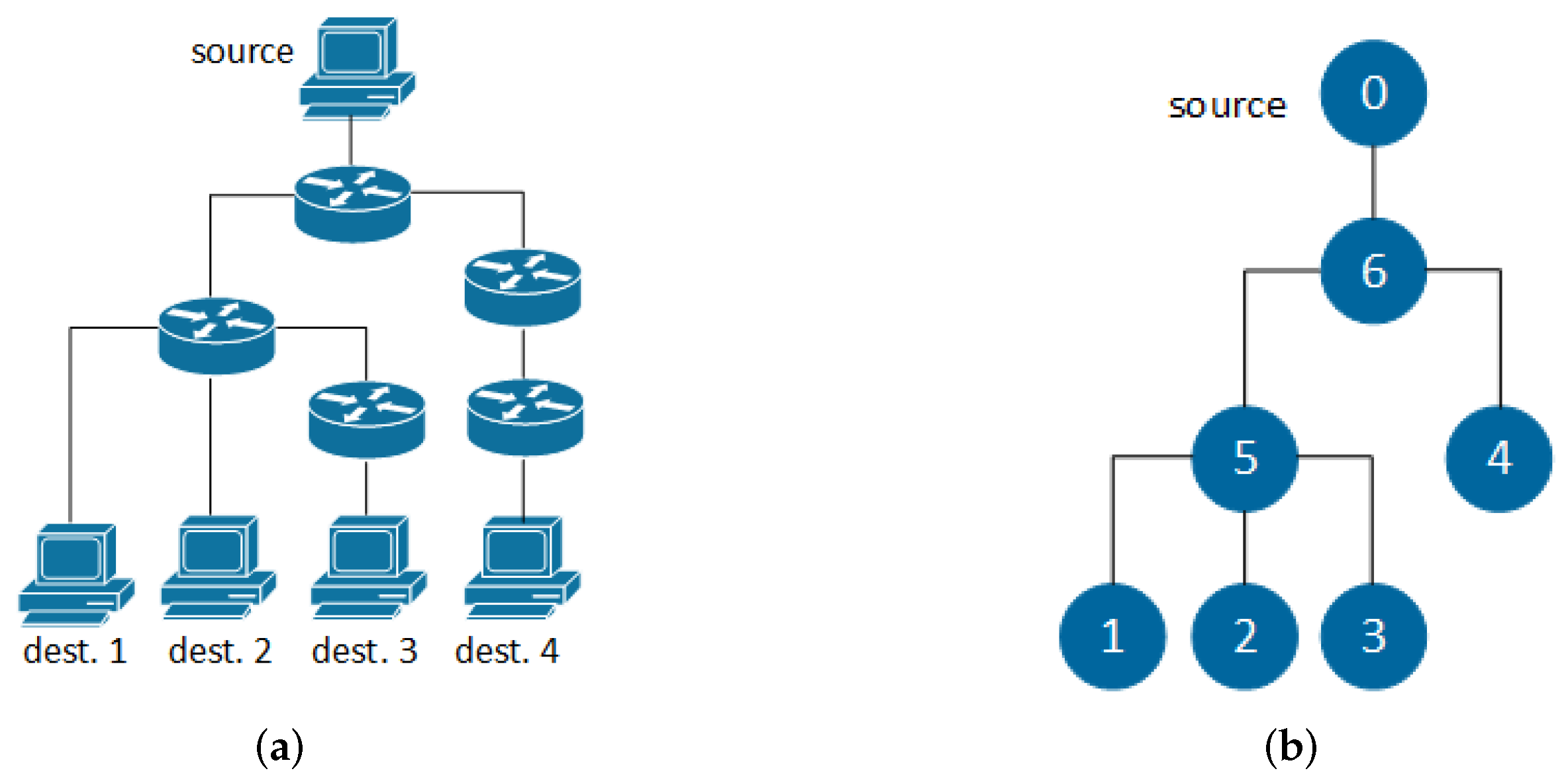
topology inference for reconstructing the topology of the network itself, which is considered unknown.
It can also be categorized as active (injecting probes) or passive (observing existing traffic), depending on the employed measurement methodology. Compared to conventional monitoring techniques that involve the direct measurement of all objects of interest, NT does not require the special-purpose cooperation of all intermediate network elements and reduces the measurement traffic overhead. In this paper, we jointly consider topology inference and link-level NT, aiming at a “minimally-required knowledge” holistic monitoring tool that needs only end-to-end measurements, obtained at the edge through active multicast probing. Our objective is to present and experimentally validate the proposed approach in a generic context, going beyond network monitoring in itself and providing a motivating example of a representative practical application of the developed clustering algorithm.
Over the years, multicast-based NT has received a lot of research attention [6,7,8,9,10]. Compared to these studies, our approach makes use of additive metrics, recovers both the unknown topology and link performance parameters, requires only the pairwise joint empirical distribution of the outcome variables at the destination nodes as input, and is easier to implement since it comprises a heuristic recursive algorithm. Furthermore, it does not employ maximum likelihood estimators, which are not computationally efficient for large-size networks because they involve finding the roots of polynomials whose degrees depend on the number of outgoing links at the internal nodes. Finally, given that the required pairwise distances between terminal nodes can be calculated using unicast packet stripe probing as well, the proposed method is not only feasible under multicast probing. The grouping algorithms presented in [11,12] are the most relevant to our work. However, by incorporating the use of nearest neighbor chains into the agglomerative clustering algorithm, we manage to further reduce the computational complexity of the proposed approach from O ( n 2 log n ) to O ( n 2 ) . Moreover, all aforementioned works infer the logical routing trees, where paths with no branches are represented as a single logical link. Contrary to that, our method can successfully identify all single-child nodes.
This work builds on [13] and provides important advances compared to what has been published so far. Although the aforementioned initial study forms the basis and the starting point of our current research, the present work has been vastly improved in terms of technical content, analysis, evaluation, and presentation, in a way that complements and significantly extends the contribution of the preliminary conference version. The main differences between the current article and the partial preliminary conference version can be briefly summarized as presenting new ideas (recovery of physical topologies, alternative reduction update formulas), additional experimentation (examining and quantifying a larger number of features and comparing with conventional tools), and a tangible application of the devised clustering algorithm. In greater detail, an important new feature of the proposed and implemented network tomography utility is the ability to infer not only logical routing trees but also the underlying physical routing trees by incorporating information about hop counts. Furthermore, we demonstrate that the reduction update formula, which is used at every iteration of the clustering algorithm for calculating the distances between the newly generated parent and the rest nodes, has a significant impact on the estimation of the link performance parameters. Taking that into consideration, we explore and experimentally compare several reduction update formulas that guarantee the correctness of the agglomerative algorithm, not being limited to only fixed schemes but also including an adaptive scheme that is tailored to the discovered hierarchy, since it depends on the number of offspring of the involved nodes. Finally, we go beyond simply presenting a modified nearest neighbor (NN) chain-extended agglomerative clustering algorithm. We design, implement, and experiment with a tangible application of the proposed inferential method that combines network tomography (NT)-based monitoring with change point analysis to realize performance anomaly detection over an actual topology constructed in an open large-scale testbed.
Overall, through the extended experimentally-driven analysis, we demonstrate the feasibility of our approach, and we provide a more detailed performance evaluation by examining and quantifying a larger number of features while also underlining a number of practical tools that can be used in the development and testing of network services. By designing, implementing, and presenting a tangible application that leverages the devised algorithm and the described extensions/modifications, we demonstrate the practical value of our approach, motivate implementation-driven deployments of similar utilities, and provide insights and good practices that can be adopted by researchers and developers working in related problems. To summarize, the key contributions of this article are the following:
  • The logical routing tree can be considered as the “skeleton” of the underlying physical topology, including only its intermediate branching points. To infer physical routing trees, we extend the nearest neighbor (NN) chain-enhanced agglomerative clustering algorithm [13] by incorporating information about hop counts.
  • The reduction update formula, which is used at every iteration for calculating the distances between the newly generated parent and the rest nodes, is a critical feature of clustering algorithms. Taking that into consideration, we explore several reduction update formulas that guarantee the correctness of the proposed algorithm, and we examine their impact on the estimation accuracy of the link performance parameters.
  • We implement the proposed clustering algorithm with all extensions and alternative options discussed in this paper, creating a complete command-line-based network tomography tool. We publish [14] the source code under a permissive free software license, along with detailed documentation.
  • We extensively evaluate the performance of the proposed algorithm, over a comprehensive set of criteria, with real topologies constructed in an open large-scale testbed.
  • We design and implement a practical application of the proposed NN-extended clustering algorithm that combines the NT-based monitoring with change point analysis for performance anomaly detection. The respective source code is also publicly available [14].
The remainder of this article is organized as follows. In Section 2, we introduce the network and probing model, along with the considered inference problem. Section 3, describes in detail the proposed algorithm, analyzes the extensions needed for inferring physical routing trees, and explores a variety of alternative reduction update formulas. In Section 4, we present the employed experimental setup and we report the respective performance evaluation results. Finally, Section 5 presents the practical application of the clustering algorithm and Section 6 concludes the paper.

2. Network Model and Problem Formulation

In this work, we focus on tree network topologies that are formed in the case of active probing from a single source. In essence, a designated root node (i.e., the source) actively sends probes to the leaves (i.e., the destination nodes), where traffic is monitored. To facilitate the collection of end-to-end measurements in our experiments using the tools described in Section 4.1, we design the examined networks with the root having only one child. The internal nodes can have exactly two children, in which case the resulting tree is binary, or two or more children, in which case the resulting tree is general. In greater detail, assuming that during the measurement period the underlying routing algorithm determines a unique path from a source to each destination that is reachable from it, the physical routing topology from a source node to a set of destination nodes is a tree called physical routing tree. The logical routing tree consists of the source node (root), the destination nodes (leaves), and the branching points (i.e., nodes with two or more outgoing links) of the physical routing tree, along with the logical links between them. Consequently, a logical link comprises a sequence of one or more consecutive physical links and the degree of every internal node of the logical routing tree is at least three. The root (i.e., source node) has only one child (therefore a degree of one), and the leaves (i.e., destination nodes) none (therefore a degree of one). Figure 1 presents an indicative topology example of both the physical and the corresponding logical routing trees.
Let T ( s , D ) = ( V , E ) denote the logical routing tree from source s to a set of destination nodes D, which consists of node set V and edge set E. Every node k V \ { s } has a parent f ( k ) V such that link e k ( f ( k ) , k ) E . Additionally, every node k V \ D has a set of children c ( k ) = { j V : f ( j ) = k } . Each link e E is associated with a performance parameter θ e (e.g., loss rate, jitter). Finally, the unique path (i.e., sequence of links) that connects nodes i and j on the logical routing tree is denoted by p ( i , j ) . The network inference problem that we consider in this paper regards using aggregate end-to-end measurements obtained at the terminal nodes (i.e., k { s } D ) for: (i) inferring the routing tree topology and (ii) estimating the fine-grained network characteristics, i.e., the individual link parameters θ e (loss rates or jitter).

2.1. Probing Model

In this work, we use source-specific multicast (SSM) due to its effectiveness and efficiency for our purposes. In particular, the multicast probing technique inherently provides sufficient packet-level correlations, which are required to infer the topology and link performance parameters. When a node receives a given multicast probe packet, it forwards a copy of the packet to its children. Therefore, the multicast packets of the same probe observed at various terminal points experience the same network conditions in their shared paths (performance contribution from links in shared paths is identical). Another advantage of multicast probing is that it can scale better compared to its unicast counterpart, given that for the latter back-to-back or even larger stripes of closely spaced unicast packets are required to emulate a multicast probe.
The main drawback of multicasting is that it is not widely deployed and readily available on the Internet. Nevertheless, as previously mentioned, the proposed algorithm can also function without any change or modification under striped unicast probing, albeit with an impact on the probing overhead scalability. The probes are only leveraged to estimate the distances between the terminal nodes, which are given as input to the algorithm. Back-to-back or even larger stripes of closely spaced unicast packets can be used to emulate a multicast probe. Of course, the emulated packet-level correlations achieved using unicast probes cannot be perfect. Therefore, multicast probing is considered the best-case experimental setting for our approach. For every probe traversing the tree, the state of each link of the routing tree is represented by the set of link state variables Y e , e E . Similarly, the set of outcome variables X k , k V denotes the (random) outcome of the probe at each node. Clearly, the outcome at node k (i.e., X k ) is determined by the outcome at the node’s parent (i.e., X f ( k ) ) and the state of the link e k = ( f ( k ) , k ) that connects them (i.e., Y e k ).

2.2. Multicast Additive Metrics

Additive link metrics are extremely important in the field of network tomography and have been widely used over the years. Under such formulations, the end-to-end measurements corresponding to paths between terminal nodes are the sums of the individual component link metrics. Delay is an example of an inherent additive link metric, whereas loss rates and other multiplicative metrics can be transformed into additive using a logarithmic scale. The network tomography inference problem can then be expressed as the inverse problem of solving the system of linear equations y = A · x , where x is the vector of unknown link parameters, A is the routing or measurement matrix representing the network topology, and y is the vector of observed path-level end-to-end measurements. The goal is to estimate the unobserved vector x given the aforementioned linear model and the known vector of measurements y . The difficulty lies in the fact that the system of linear equations is heavily under-determined.
Using the previously described notation, an additive metric d : V × V R + on tree T = ( V , E ) is a non-negative function such that:
  • 0 < d ( e ) < , e E ,
  • d ( i , j ) = 0 if and only if i = j , and
  • d ( i , j ) = d ( j , i ) = e p ( i , j ) d ( e ) , otherwise.
The topology and the link lengths d ( e ) , e E of a tree T ( s , D ) = ( V , E ) can be recovered by the pairwise distances D = { d ( i , j ) : i , j { s } D } between the terminal nodes under an additive metric [15]. Assuming that the link states are independent and stationary during the measurement period, we can construct the following additive metrics:
  • d ( e ) = log ( θ e ) , e E , where θ e is the success rate (i.e., the complement of loss rate) of link e.
  • d ( e ) = θ e = Var Y e , e E , where Y e is a random variable that expresses the random queuing delay of link e and θ e is the square of jitter of link e, with jitter defined as the standard deviation of delay σ ( Y e ) in order to be additive.
In the first case, the link-state variable Y e is equal to one (or zero) with probability θ e (or 1 θ e ), if the probe traverses successfully (or is lost on) link e, and the outcome variable X k takes value 1, if the probe reaches node k, and value 0 otherwise. Then, the outcome variable at a particular node can be expressed as the product of the link-state variables corresponding to the links comprising the path from the source to that specific node. Furthermore, the probability that this outcome variable takes value one can be computed as the product of the success rates corresponding to the links along that same path. Therefore, we can construct an additive tree metric with a link length equal to the negative logarithm of the complement of the packet loss rate. In the second case, the link-state variable Y e expresses the random queuing delay of link e and the outcome variable X k represents the cumulative end-to-end queuing delay that is experienced by the probe on its way to node k. Then, the outcome variable at a particular node can be expressed as the sum of the link-state variables corresponding to the links comprising the path from the source to that specific node. Moreover, given that the variance of a sum of independent random variables is the sum of their variances, the variance of this outcome variable can be computed as the sum of the performance parameters associated with the links along that same path. Consequently, we can construct an additive tree metric with a link length equal to the square of jitter. Accordingly, the pairwise distances between the terminal nodes for the aforementioned additive metrics can be calculated as follows [13]:
d ( s , i ) = log 1 P X i = 1 = log P X i = 1 , i D
d ( i , j ) = log P X i = 1 · P X j = 1 P X i X j = 1 2 , i , j D
for the loss-based metric, and
d ( s , i ) = Var X i , i D
d ( i , j ) = Var X i + Var X j 2 · Cov X i , X j , i , j D
for the delay-based metric. Assuming source s sends n probes to the destination nodes D, the outcome variables at the terminal nodes
X k ( t ) : k { s } D and t = 1 , 2 , , n
can be observed. Then, according to the employed additive metric, we can estimate the above pairwise distances leveraging the fact that the maximum likelihood estimator (MLE) of the probability that a Bernoulli random variable takes value one is equal to the sample mean and using the unbiased sample variance (with lost packets ignored) as follows:
d ^ ( s , i ) = log X i ¯
d ^ ( i , j ) = log X i ¯ · X j ¯ X i X j ¯ 2 , i , j D
for the loss-based metric, and
d ^ ( s , i ) = Var ^ X i , i D
d ^ ( i , j ) = Var ^ X i + Var ^ X j 2 Cov ^ X i , X j , i , j D
for the delay-based metric, where
X i ¯ = 1 n t = 1 n X i ( t ) , X i X j ¯ = 1 n t = 1 n X i ( t ) X j ( t ) ,
Var ^ X i = 1 n 1 t = 1 n X i ( t ) X i ¯ 2 , and
Cov ^ X i , X j = 1 n 1 t = 1 n X i ( t ) X i ¯ X j ( t ) X j ¯ .

3. Topology Inference and Estimation of Link Parameters

In this section, we present in detail the nearest neighbor (NN) chain-extended agglomerative clustering algorithm and the modifications/extensions we incorporate to fulfill our objectives.

3.1. Distance-Based Agglomerative Hierarchical Clustering

In order to infer the logical routing tree using the estimated pairwise distances between terminal nodes under the previously described additive metrics, we employ an agglomerative hierarchical clustering algorithm with O ( n 2 ) complexity [13], where n is the number of network nodes. Furthermore, given that there is a one-to-one mapping between the returned edge lengths d ( e ) , e E and the underlying link performance parameters θ e , e E (see Section 2.2), we can also estimate the latter from the former as follows:
  • loss rate of link e = 1 θ e = 1 10 d ( e ) , and
  • jitter of link e = θ e = d ( e ) , e E .
Broadly speaking, the employed clustering algorithm operates in a bottom-up manner, starting with a set including all destination nodes, each one in its own cluster, and selecting at each iteration two nodes that are joined and replaced in the set by a new node designated as their parent. This process continues recursively on this reduced set until there is only one node left, which will be the (single) child of the root (source) s. A high-level overview of the algorithm is presented in Figure 2.
In the following, we discuss the specifics of the functionality and the detailed operation of each depicted step:
  • The input of the algorithm is the source node s, the set of destination nodes D, and the estimated pairwise distances between terminal nodes D ^ = { d ^ ( i , j ) : i , j { s } D } , calculated as described in Section 2.2.
  • The output of the algorithm is the logical routing tree T ( s , D ) = ( V , E ) and the link lengths d ( e ) , e E , from which we can obtain the link parameters θ e , e E .
  • At initialization, we start by adding the source and the destinations to the set of nodes, V = { s } D , and we initialize the set of edges equal to the empty set, E = .
  • For every pair of nodes i and j of the routing tree, the lowest common ancestor, LCA ( i , j ) , is the node that is located the farthest from the root and has both nodes as descendants. The depth of the lowest common ancestor, ( i , j ) = d ( s , LCA ( i , j ) ) , expresses the length of the shared path from s to i and j. Given that there is a one-to-one mapping between the pairwise distances and the LCA depths, we can equivalently employ the latter to infer the routing tree and estimate the link parameters. To that end, at the step construction of LCA depths matrix, we compute the | D | × | D | matrix of LCA depths L = ( i , j ) , i , j D using the equations
    ( i , j ) = 1 2 [ d ( s , i ) + d ( s , j ) d ( i , j ) ] , i , j D and
    ( i , i ) = d ( s , i ) , i D .
  • At the neighbor selection step, we choose the two nodes that are deemed siblings and are about to be joined. Taking into account that the LCA depth of two nodes expresses the length of their shared path, we select the nodes i and j that are mutual or reciprocal nearest neighbor (RNNs), meaning that, for each one, their LCA depth is the largest among all others: k i , j , ( i , j ) ( i , k ) , ( j , k ) . The idea is that two siblings must have the largest shared path with one another, compared to all other nodes. Such RNNs can be found efficiently by constructing nearest neighbor (NN) chains [16]. Essentially, a NN chain follows paths in the nearest neighbor graph of the clusters, until the paths terminate in a pair of RNNs. It starts at an arbitrary initial node, and it is iteratively extended from the current node at the top of the chain, say i, to its nearest neighbor j such that ( i , j ) = max k i ( i , k ) , until it necessarily terminates at a pair of RNNs. After joining the discovered RNNs, the rest NN chain is still valid and, therefore, it is not discarded. Each node (either destination or intermediate created parent) enters the NN chain only once, where it remains until it is joined with another node.
  • At reduction step, we create node u as the parent of the previously found RNNs i and j, and we calculate its LCA depth with the remaining nodes ( u , k ) , k D , k u , i , j . The choice of the employed reduction update formula is a crucial issue, which we analyze in Section 3.3.
  • Tree reconstruction regards the update of the data structures related to the part of the tree that has been recovered up to this moment. In greater detail, we remove the found RNNs i and j from set D, D = D \ { i , j } ; we add the newly created parent node u to sets V and D, V = V { u } and D = D { u } ; we add the two new edges to set E, E = E { ( u , i ) , ( u , j ) } ; and we connect i and j to u with link lengths d ( u , i ) = ( i , i ) ( i , j ) and d ( u , j ) = ( j , j ) ( i , j ) .
  • Finally, if there is only one node left in set D (stopping condition | D | = 1 ), we connect that remaining node with the source and we terminate the algorithm, otherwise we return to the neighbor selection step and we repeat the process.
Given that a pair of RNNs is selected as siblings at every iteration, the output of the algorithm will be a binary inferred tree. To successfully apply the algorithm to general routing trees, nodes can be grouped as if the tree was binary, and then the “extra” edges of approximately zero length (excluding the edge between the root and its single child) can be removed at a post-processing step.

3.2. Inferring Physical Routing Trees

As previously mentioned, the output of the algorithm presented in Section 3.1 is the logical routing tree, which consists of the branching points of the physical topology. However, internal nodes where no branching of traffic occurs (i.e., nodes with a single child) do not appear in the logical tree and long paths with no branches might be represented as a single logical link. Therefore, the logical tree might differ significantly from the underlying physical routing tree. To infer more accurately the physical routing tree, in this work we incorporate into the algorithm information regarding the number of hops needed for reaching each node starting from the source. Assuming that we only have access to the network edge and not to the internal nodes, such information can be readily obtained simply by capturing the employed probes at the destination nodes using a packet analyzer tool and examining their time-to-live (TTL) fields. The idea is that two nodes that are siblings must have the same TTL value. At each iteration, the TTL value of the newly created parent of the selected RNNs is calculated based on the TTL value of its children.
In more detail, we start by extracting the TTL values corresponding to each destination node from the realized end-to-end measurements. Then, we modify the neighbor selection step as follows. After selecting a pair of RNNs, we check the respective TTL values of the two nodes. If they are equal, we proceed to the next step. Otherwise, we can deduce that the node with the smaller TTL value is located in a path with no branching points. To rectify this, we assign this node as the single child of a newly created parent, with a properly adjusted TTL value (i.e., incremented by one). We continue adding such parent nodes until the new TTL value becomes equal to that of the other RNN. Following that in the next step, we properly set (i.e., increment by one) the TTL value of the node that is designated as the parent of the two siblings (i.e., the two RNNs in the first case, or the head of the no branching path and the remaining RNN in the second case), and we proceed to the rest of the algorithm as before.

3.3. Reduction Update Formulas

Contrary to the conventional greedy agglomerative approach that repeatedly joins the two overall “closest” nodes (in our context, the nodes with the overall largest LCA depth), the proposed NN chain-enhanced algorithm joins any pair of RNNs as it is found. Consequently, the order of the cluster merges might be different. However, provided that the reduction update formula satisfies two certain properties, the resulted hierarchy will be the same [17]. Such suitable reduction update schemes are:
  • the single reduction update formula:
    ( u , k ) = min { ( i , k ) , ( j , k ) }
  • the complete reduction update formula:
    ( u , k ) = max { ( i , k ) , ( j , k ) }
  • the average reduction update formula:
    ( u , k ) = 1 n i + n j n i · ( i , k ) + n j · ( j , k )
  • the weighted reduction update formula:
    ( u , k ) = 1 2 ( i , k ) + ( j , k )
k D , k u , i , j , where i and j are the pair of RNNs, u is the newly created parent, and n i , n j , n k are the sizes of clusters i, j and k, which in our context can be interpreted as the number of the descendants of the respective nodes. As can be seen, the single, complete, and weighted schemes are “conservative” in the sense that they are fixed and do not adapt to the discovered hierarchy, whereas the average scheme depends also on the number of offspring of the involved nodes, thus being better tailored to each particular case. In [13], the use of the weighted and complete update formulas has been examined. Here, we comparatively explore all of the aforementioned schemes, as well as the generic convex formula analyzed in Section 4.2.

4. Performance Evaluation

The experiments presented in this article take place in a fully-controlled testbed to demonstrate the feasibility of our ideas. Exploring how our methods can be further fine-tuned and adapted to specific types of networks (e.g., cloud, overlay, or data center networks) and their particular characteristics is left for future work.

4.1. Experimental Setup

To evaluate the performance of the proposed algorithm in topology inference and estimate the link loss rates and jitter, we constructed several binary (i.e., all internal nodes have exactly two children) and general (i.e., internal nodes have two or more children) physical routing trees, following the network model described in Section 2, over bare-metal hardware in the Virtual Wall [18] testbed of the Fed4FIREPlus [19] federation. Routing was realized using the Quagga software suite and network impairment (i.e., loss and jitter) on links were configured on software using the netem kernel module and the tc utility. In particular, we employed the ospfd and pimd quagga routing daemons, implementing the OSPF, PIM-SSM, and IGMP protocols, while the links’ loss rates and jitter values were chosen in the ranges 0–20% and 0–400 ms, respectively. The iperf traffic tool was used for performing multicast active probing and the required end-to-end measurements were obtained at the outgoing interface of the source node and the incoming interfaces of the destination nodes using the tcpdump command-line packet analyzer. For every routing tree, three different numbers of probes were examined, namely probes 2128, 5105, and 10,207.

4.2. Results and Discussion

The command-line network tomography tool has been developed in Python 3 and accepts as arguments the tcpdump output (since we do not need the detailed content of probe packets, we do not use pcap files) captured at the outgoing link of the source and the incoming links of the destinations. The binary routing trees are inferred correctly for all the conducted experimental scenarios. The extension of the algorithm to general routing trees is somewhat more complicated since it requires the selection of a suitable threshold that may vary from case to case due to the accumulated estimation errors of link lengths. For every examined experimental scenario, there is a fitting threshold under which the general routing tree is reconstructed correctly. However, in practice, it is more realistic to use a single predetermined hard-coded threshold. In this case, 48 out of 48, and 36 out of 48 experimental configurations (i.e., combinations of topology type, number of probes, and reduction update scheme) result in a correctly recovered tree under the loss-based metric and the jitter-based metric, respectively.
Table 1 lists the aggregated errors of the conducted experiments, to evaluate the accuracy of the link performance parameter estimation for several physical routing trees. The first column indicates the type of the studied topology (either binary or general physical routing tree) and the number of its nodes. The rest columns present the aggregated estimation errors of the respective test networks for each examined reduction update formula presented in Section 3.3 and for three different numbers of multicast probes (namely, 2128, 5105, and 10,207 probes) generated using iperf. In particular, we calculate and report the Root Mean Square Error (RMSE) for every experimental scenario (i.e., combination of topology, employed reduction formula, and the number of probes) according to the following equation:
RMSE = 1 | E | 1 e E \ { ( s , c ( s ) ) } y e y ^ e 2
where y ^ e is the estimate of the loss rate (or jitter) of link e, and y e is the respective ground truth (i.e., the argument of tc). In other words, we consider the arguments that we passed to the tc utility during the experimental setup as the ground truth for the actual values of the links‘ loss rates and jitter that are compared to the estimations returned by our model. Loss rates are written as percentages, and jitter is measured in milliseconds. As can be seen, even though the estimation accuracy improves as the number of employed probes increases, the reported errors are relatively small for all configurations. Furthermore, despite being one of the “fixed” schemes, the weighted formula gives the better estimations for the majority of the experiments, followed closely by the average scheme, the only “adaptive” option.
Conventional network monitoring tools based on traditional IP-based mechanisms (e.g., ping, traceroute) are device-centric hop-by-hop approaches that rely on exchanging traffic (e.g., ICMP packets) with intermediate nodes and involve the direct measurement and observation of all entities of interest. Consequently, they require the special-purpose cooperation and participation of all network elements, which is not always feasible in large-scale IP networks due to administrative or security considerations (e.g., many nodes are configured to ignore ICMP packets altogether). Additionally, contrary to the proposed inferential approach, they assume knowledge of the exact topology of the examined network. Another important benefit of the presented NT-based method compared to traditional tools is the ability to provide a global overview of the network state without collecting fine-grained individual statistics but using end-to-end measurements realized at the network edge. As such, it reduces the computational and traffic overhead of the measurement process by decreasing the generated probing load and the consumption of valuable network resources (e.g., bandwidth, CPU, and memory).
Assuming ideal conditions for the conventional tools (i.e., a priori known topology and unobstructed access to all intermediate nodes) and focusing only on link parameter estimation, we demonstrate the relation between measurement overhead and estimation accuracy for the NT-based approach and a representative conventional monitoring tool by selecting the general physical routing tree topology with 10 nodes and measuring the links‘ loss rates with the iperf tool using UDP probes (running an iperf server and client at the endpoints of the links). In particular, iperf was configured to send 1022, 1532, and 2042 probes at each link, resulting in 8176, 12,256, and 16,336 probes in total over the entire network. The achieved RMSE (the average of three measurements) was 0.5970 , 0.4277 , and 0.3335 , respectively. As can be seen by comparing the respective results listed in Table 1, our approach can yield comparable estimation errors while utilizing a smaller number of probes, even in such a small-scale sample network.
In order to demonstrate the impact of the reduction update scheme to the estimation accuracy, we consider the following generic formula:
( u , k ) = α ( i , k ) + ( 1 α ) ( j , k ) , with 0 α 1 , k D , k u , i , j .
Equation (16) can be employed during the reduction step of the clustering algorithm to compute the LCA depth of the newly created parent node u with every other node k as a convex combination of the LCA depths of that node with the two selected RNNs (i.e., nodes i and j). Since the coefficients of a convex combination must be non-negative and must sum to 1, in our case, α takes a value within the range 0–1. We select one of the experimental scenarios (Bin. 32) and we plot the resulting RMSE in relation to the value of α (Figure 3) under the loss-based metric. As can be seen, the error varies significantly as the employed update formula changes. In this particular case, it appears that the best result is obtained for α = 0.79 .
Finally, Table 2 lists the execution time (in seconds) for the various experimental scenarios, as recorded in a reference machine with the following specifications: Intel Core i5-6500 @4x 3.6 GHz CPU and 16 GB DDR4 2133 MHz RAM. These measurements were taken using 5105 multicast probes, which were transmitted in 60 s (a time period that is not considered in this table). As it is evident, although no special optimizations have been made to that end, the required times are indeed rather small and depend on the size of the examined topology (the differences between alternative configurations applied to each examined tree are negligible). Nevertheless, an implementation in a compiled language is expected to further reduce the execution time, if so desired.

5. Motivating Detection Application

As previously mentioned, one of the main objectives of this work is to go beyond validating the feasibility of the proposed clustering algorithm to designing, implementing, and presenting an actual application that leverages the devised inferential monitoring approach for performing a tangible task in a real testing network. The reasons for pursuing this direction are manifold:
  • We want to demonstrate the practical value of our technical content and point out that it is not limited to theoretical contributions.
  • We aim to motivate the adoption and further extension of our methods by researchers and developers working on related problems by providing a ready-to-use open-source implementation of an NT-enabled network service.
  • We try to highlight some representative tools and outline the overall process that can be followed for performing validation trials and experiments with real equipment.
Monitoring and identifying unusual or anomalous activity is essential for ensuring the efficient operation of network infrastructures. Hereinafter, we combine the proposed clustering algorithm with change point analysis [20] for detecting the occurrence of performance anomalies (i.e., abrupt changes to loss events). The topology employed in our experiments is illustrated in Figure 4, and for change point detection we have leveraged the methods provided by the ruptures [21] library. In particular, the approach we follow consists of the following steps:
(i)
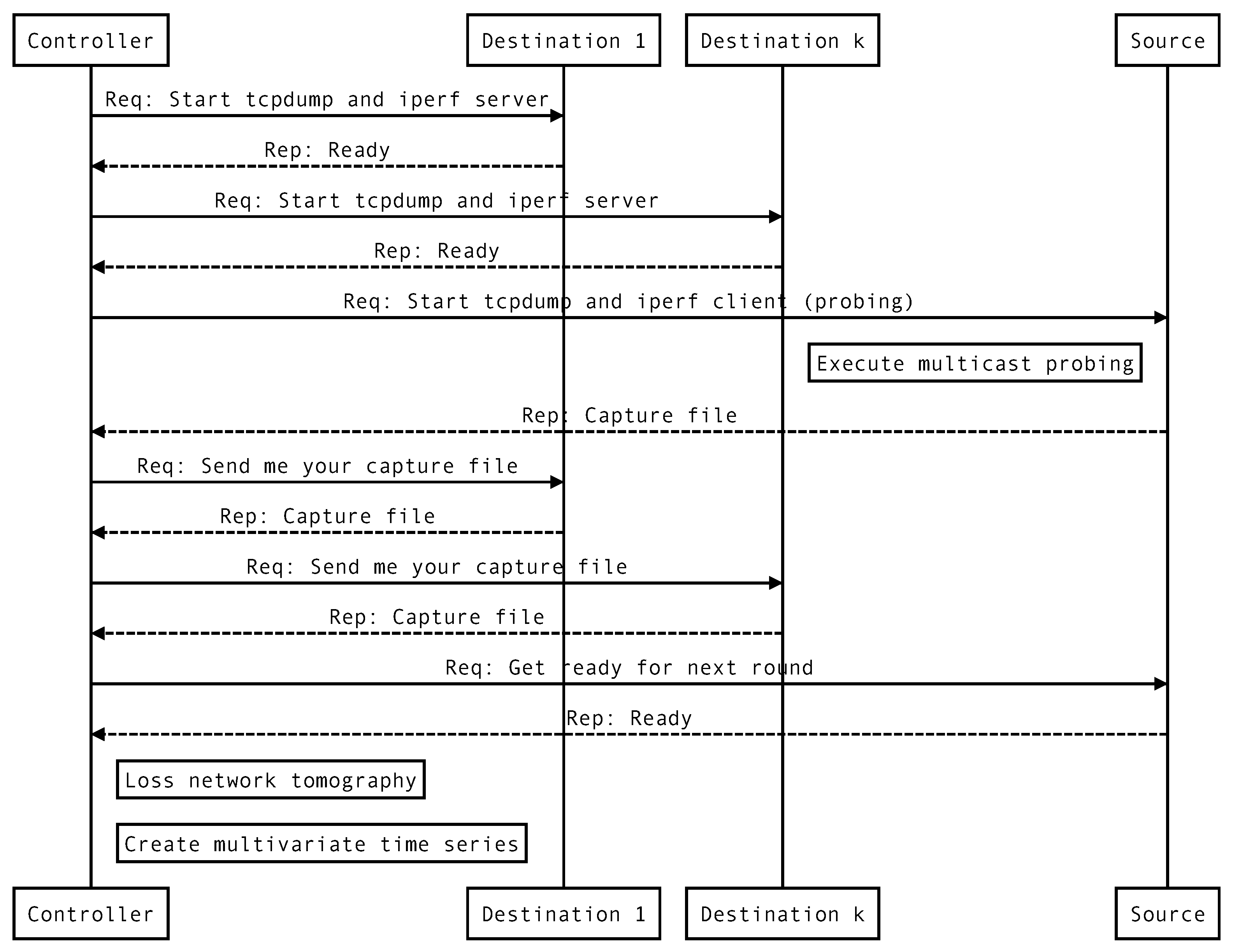
execute active multicast probing at the periphery of the network,
(ii)
apply the NN-extended clustering algorithm to estimate the loss rates of all links,
(iii)
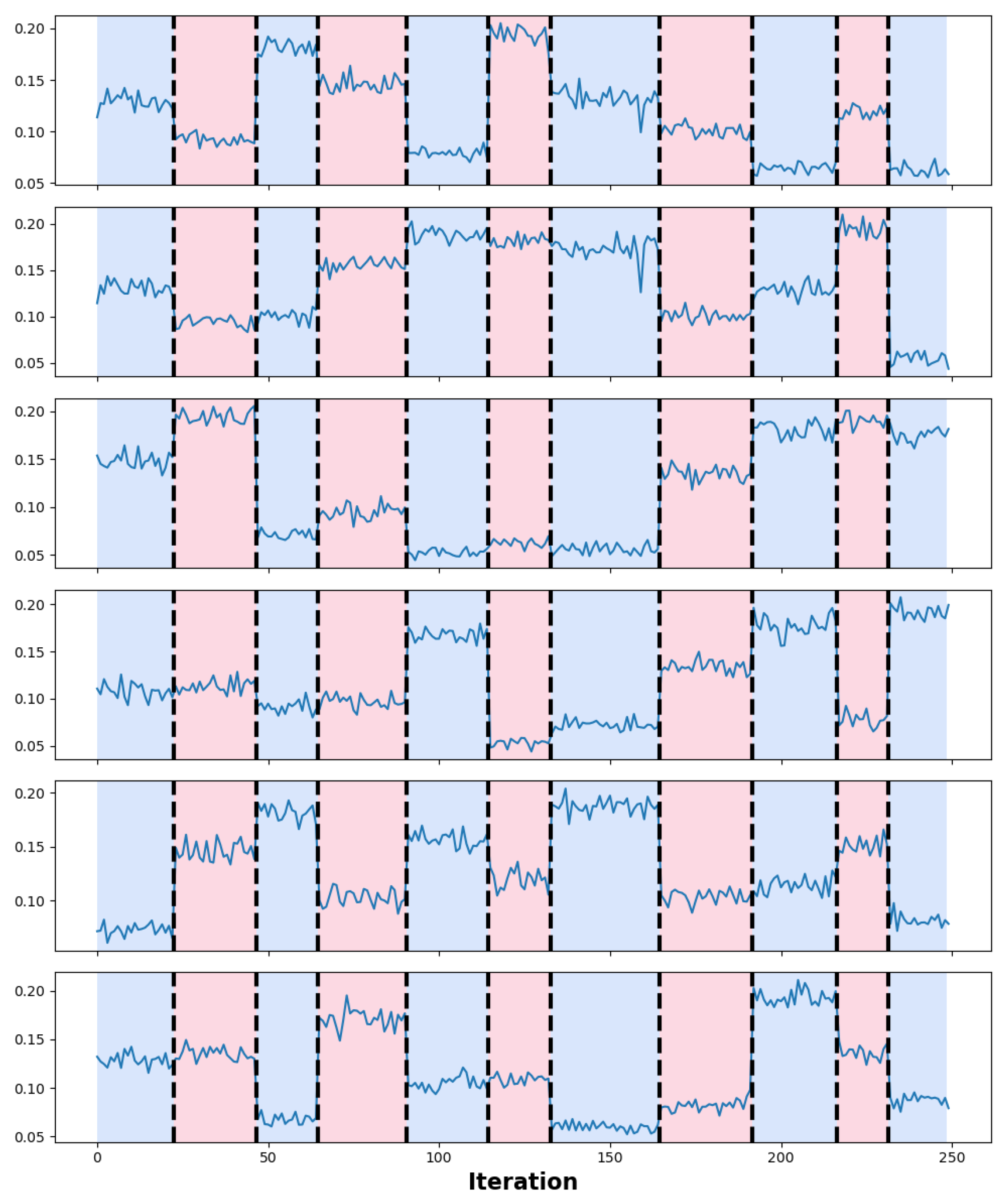
repeat the previous two steps at regular intervals/rounds and record the obtained estimates in a multivariate time series, and
(iv)
perform offline change point analysis on the multivariate time series to detect the breakpoints, i.e., the rounds where the loss rates’ distribution changes significantly.
To coordinate the probing process and the required traffic captures, a node that can reach all terminal nodes is appointed as a controller. This controller is also charged with collecting all capture files and estimating the links’ loss rates via network tomography at every round/iteration, to create a multivariate time series. The interactions between the controller and the terminal nodes (i.e., source and destinations) in every round/iteration are depicted in Figure 5. All communications between the nodes are realized with the ZeroMQ [22] asynchronous messaging library (following the request-reply messaging pattern) and, after constructing the multivariate time series, the linearly penalized segmentation (Pelt) algorithm [23] is employed for detecting the change points.
Figure 6 illustrates the loss rate estimates for every link of the topology (obtained using the proposed algorithm) across 250 iterations/rounds. The change of color indicates the real breakpoints (i.e., the iterations when the underlying distribution of the links’ loss rates was changed during the experiment—the ground truth) and the dashed lines denote the breakpoints that were detected by applying the offline change-point algorithm to the obtained estimates. As can be seen, the two sets of breakpoints are indistinguishable.

6. Conclusions

In this article, we presented and implemented a clustering algorithm for performing inferential network monitoring based on multicast end-to-end measurements. Specifically, we addressed the problems of inferring the routing tree topology (both logical and physical) and estimating two link performance parameters (i.e., loss rate and jitter). The experimental results regarding the accuracy and the execution time of the proposed algorithm, as well as the presented motivating application leveraging change point analysis, demonstrated its promising potential as a close to real-time monitoring tool and an enabler of performance anomaly detection.
Regarding future work, we plan to explore and experimentally validate more applications of the proposed NT monitoring approach. One such example is the development of a utility-based framework enabling advanced decision-making. The envisaged utility function can incorporate network-centric QoS parameters provided and updated by the clustering algorithm to promote informed decisions based on network utility maximization.

Author Contributions

All authors contributed to the conceptualization of the paper. G.K. and V.K. outlined the structure of the article. G.K. was responsible for software development, performance evaluation, and preparation of the original draft. V.K. and S.P. performed the critical review and overall consistency check. All authors have read and agreed to the published version of the manuscript.

Funding

This work was supported by the European Commission in the framework of the H2020-ICT-19-2019 project 5G-HEART (Grant Agreement No. 857034).

Data Availability Statement

Not Applicable, the study does not report any data.

Conflicts of Interest

The authors declare no conflict of interest.

Abbreviations

The following abbreviations are used in this manuscript:
INTIn-band Network Telemetry
PFEProgrammable Forwarding Engine
SDNSoftware Defined Networking
NTNetwork Tomography
QoSQuality of Service
ODOrigin-Destination
NNNearest Neighbor
SSMSource-Specific Multicast
MLEMaximum Likelihood Estimator
LCALowest Common Ancestor
RNNsReciprocal Nearest Neighbor
TTLTime-To-Live
RMSERoot Mean Square Error

References

  1. Haxhibeqiri, J.; Isolani, P.H.; Marquez-Barja, J.M.; Moerman, I.; Hoebeke, J. In-Band Network Monitoring Technique to Support SDN-Based Wireless Networks. IEEE Trans. Netw. Serv. Manag. 2021, 18, 627–641. [Google Scholar] [CrossRef]
  2. Sonchack, J.; Michel, O.; Aviv, A.J.; Keller, E.; Smith, J.M. Scaling Hardware Accelerated Network Monitoring to Concurrent and Dynamic Queries with *Flow. In Proceedings of the 2018 USENIX Annual Technical Conference (USENIX ATC 18), Boston, MA, USA, 11–13 July 2018; pp. 823–835. [Google Scholar]
  3. Kakkavas, G.; Stamou, A.; Karyotis, V.; Papavassiliou, S. Network Tomography for Efficient Monitoring in SDN-Enabled 5G Networks and Beyond: Challenges and Opportunities. IEEE Commun. Mag. 2021, 59, 70–76. [Google Scholar] [CrossRef]
  4. Kakkavas, G.; Gkatzioura, D.; Karyotis, V.; Papavassiliou, S. A Review of Advanced Algebraic Approaches Enabling Network Tomography for Future Network Infrastructures. Future Internet 2020, 12, 20. [Google Scholar] [CrossRef] [Green Version]
  5. Kakkavas, G.; Kalntis, M.; Karyotis, V.; Papavassiliou, S. Future Network Traffic Matrix Synthesis and Estimation Based on Deep Generative Models. In Proceedings of the 2021 International Conference on Computer Communications and Networks (ICCCN), Athens, Greece, 19–22 July 2021. [Google Scholar] [CrossRef]
  6. Caceres, R.; Duffield, N.G.; Horowitz, J.; Towsley, D.F. Multicast-based inference of network-internal loss characteristics. IEEE Trans. Inf. Theory 1999, 45, 2462–2480. [Google Scholar] [CrossRef] [Green Version]
  7. Duffield, N.; Horowitz, J.; Presti, F.L.; Towsley, D. Multicast topology inference from measured end-to-end loss. IEEE Trans. Inf. Theory 2002, 48, 26–45. [Google Scholar] [CrossRef]
  8. Presti, F.L.; Duffield, N.; Horowitz, J.; Towsley, D. Multicast-based inference of network-internal delay distributions. IEEE/ACM Trans. Netw. 2002, 10, 761–775. [Google Scholar] [CrossRef] [Green Version]
  9. Liang, G.; Yu, B. Maximum pseudo likelihood estimation in network tomography. IEEE Trans. Signal Process. 2003, 51, 2043–2053. [Google Scholar] [CrossRef]
  10. Duffield, N.; Horowitz, J.; Presti, F.L.; Towsley, D. Explicit Loss Inference in Multicast Tomography. IEEE Trans. Inf. Theory 2006, 52, 3852–3855. [Google Scholar] [CrossRef]
  11. Ni, J.; Xie, H.; Tatikonda, S.; Yang, Y. Efficient and Dynamic Routing Topology Inference from End-to-End Measurements. IEEE/ACM Trans. Netw. 2010, 18, 123–135. [Google Scholar] [CrossRef]
  12. Ni, J.; Tatikonda, S. Network Tomography Based on Additive Metrics. IEEE Trans. Inf. Theory 2011, 57, 7798–7809. [Google Scholar] [CrossRef]
  13. Kakkavas, G.; Karyotis, V.; Papavassiliou, S. A Distance-based Agglomerative Clustering Algorithm for Multicast Network Tomography. In Proceedings of the ICC 2020—2020 IEEE International Conference on Communications (ICC), Dublin, Ireland, 7–11 June 2020. [Google Scholar] [CrossRef]
  14. Kakkavas, G. Inferential Network Monitoring. Available online: https://gitlab.com/gkakkavas/lca-rnn-extension (accessed on 7 January 2022).
  15. Buneman, P. The Recovery of Trees from Measures of Dissimilarity. In Mathematics the Archeological and Historical Sciences; Edinburgh University Press: Edinburgh, UK, 1971; pp. 387–395. [Google Scholar]
  16. Murtagh, F.; Contreras, P. Algorithms for hierarchical clustering: An overview, II. WIREs Data Min. Knowl. Discov. 2017, 7. [Google Scholar] [CrossRef] [Green Version]
  17. Müllner, D. Modern hierarchical, agglomerative clustering algorithms. arXiv 2011, arXiv:1109.2378. [Google Scholar]
  18. Virtual Wall. Available online: https://doc.ilabt.imec.be/ilabt/virtualwall/ (accessed on 7 January 2022).
  19. Federation For Fire Plus. Available online: https://www.fed4fire.eu/ (accessed on 7 January 2022).
  20. Aminikhanghahi, S.; Cook, D.J. A survey of methods for time series change point detection. Knowl. Inf. Syst. 2016, 51, 339–367. [Google Scholar] [CrossRef] [PubMed] [Green Version]
  21. Truong, C.; Oudre, L.; Vayatis, N. Selective review of offline change point detection methods. Signal Process. 2020, 167, 107299. [Google Scholar] [CrossRef] [Green Version]
  22. Hintjens, P. ØMQ—The Guide. Available online: https://zguide.zeromq.org/ (accessed on 5 January 2022).
  23. Killick, R.; Fearnhead, P.; Eckley, I.A. Optimal Detection of Changepoints with a Linear Computational Cost. J. Am. Stat. Assoc. 2012, 107, 1590–1598. [Google Scholar] [CrossRef]
Figure 1. Example of corresponding physical and logical routing trees. (a) Physical routing tree. (b) Logical routing tree.
Futureinternet 14 00045 g001
Figure 2. High-level overview of the proposed clustering algorithm.
Futureinternet 14 00045 g002
Figure 3. RMSE for different values of α .
Futureinternet 14 00045 g003
Figure 4. Employed experimental topology.
Futureinternet 14 00045 g004
Figure 5. Sequence diagram of the interactions among the nodes in one round.
Futureinternet 14 00045 g005
Figure 6. Loss rate estimates and detected change points.
Futureinternet 14 00045 g006
Table 1. Estimation errors of the conducted experimental scenarios.
PhysicalSingleCompleteAverageWeighted
Routing Tree2k5k10k2k5k10k2k5k10k2k5k10k
Type# NdsRoot Mean Square Error for Loss Rate Estimation (%)
Bin.80.63690.48590.38790.58920.37140.40610.61240.42480.39610.61240.42480.3961
Bin.161.18240.60660.44311.84910.74920.43331.23460.64960.39121.21890.64420.3902
Bin.241.24860.49240.40861.28590.56430.49391.12970.48810.41521.13930.50870.3963
Bin.321.56780.97900.72261.56920.95420.55881.17490.84230.46491.19800.83540.4399
Gen.100.77980.33350.46090.77870.31720.63940.68260.31800.52380.66270.31770.5357
Gen.201.15710.50120.33540.96760.69720.36400.93340.53980.30790.87700.53440.3173
Gen.300.91280.58670.61080.88890.54760.46230.73080.51690.47070.74320.51570.4718
Gen.401.23800.81340.64061.29770.83680.69241.05570.69500.51111.14510.65970.5120
Type# NdsRoot Mean Square Error for Jitter Estimation (ms)
Bin.82.28842.26251.88292.48402.34501.97472.35892.28911.91222.35892.28911.9122
Bin.1610.79575.11863.38337.55244.74074.00487.71354.78553.61107.15544.72763.3867
Bin.249.07895.24344.03068.90494.72183.47567.74044.75453.62217.64454.69653.4926
Bin.3213.47037.41444.430614.628510.14436.535710.93087.04544.343811.05756.79054.4002
Gen.101.98351.54221.40803.63591.55461.54691.86891.33501.46102.10251.36071.4249
Gen.207.76154.56663.22019.32035.88373.85646.08764.79763.16585.78664.72193.1139
Gen.307.35996.00903.252312.82258.39695.19317.41525.29173.52436.83745.26163.4022
Gen.4011.80776.43435.035214.03487.72536.796910.39505.24124.422210.26115.14724.2874
Table 2. Execution time of experimental scenarios.
Physical TreeSingleCompleteAverageWeighted
Type# NdsLoss Rate Estimation Execution Time (s)
Bin.80.26650.26140.25920.2645
Bin.160.30050.30420.29880.2989
Bin.240.39500.39400.40080.3976
Bin.320.46260.45860.45780.4555
Gen.100.28790.28470.28760.2878
Gen.200.36690.36550.36990.5344
Gen.300.47970.48570.47980.4793
Gen.400.53460.52850.53570.5281
Type# NdsJitter Estimation Execution Time (s)
Bin.80.32290.32570.32120.3272
Bin.160.44590.45150.44590.4448
Bin.240.68000.68710.68030.6816
Bin.320.90270.90210.91270.9140
Gen.100.38230.37830.38300.3809
Gen.200.65140.66200.66680.6620
Gen.301.01721.01431.01891.0104
Gen.401.34131.34351.34961.3294
Publisher’s Note: MDPI stays neutral with regard to jurisdictional claims in published maps and institutional affiliations.

