Article

Real-Time Detection of Vine Trunk for Robot Localization Using Deep Learning Models Developed for Edge TPU Devices

by
Khadijeh Alibabaei
1,2,*,
Eduardo Assunção
1,2,
Pedro D. Gaspar
1,2,
Vasco N. G. J. Soares
3,4,* and
João M. L. P. Caldeira
3,4
1
Department of Electromechanical Engineering, University of Beira Interior, 6201-001 Covilhã, Portugal
2
Centre for Mechanical and Aerospace Science and Technologies (C-MAST), University of Beira Interior, 6201-001 Covilhã, Portugal
3
Polytechnic Institute of Castelo Branco, 6000-084 Castelo Branco, Portugal
4
Instituto de Telecomunicações, 6201-001 Covilhã, Portugal
*
Authors to whom correspondence should be addressed.
Future Internet 2022, 14(7), 199; https://doi.org/10.3390/fi14070199
Submission received: 1 June 2022 / Revised: 28 June 2022 / Accepted: 28 June 2022 / Published: 29 June 2022
(This article belongs to the Special Issue Advances in Agriculture 4.0)

Abstract

:
The concept of the Internet of Things (IoT) in agriculture is associated with the use of high-tech devices such as robots and sensors that are interconnected to assess or monitor conditions on a particular plot of land and then deploy the various factors of production such as seeds, fertilizer, water, etc., accordingly. Vine trunk detection can help create an accurate map of the vineyard that the agricultural robot can rely on to safely navigate and perform a variety of agricultural tasks such as harvesting, pruning, etc. In this work, the state-of-the-art single-shot multibox detector (SSD) with MobileDet Edge TPU and MobileNet Edge TPU models as the backbone was used to detect the tree trunks in the vineyard. Compared to the SSD with MobileNet-V1, MobileNet-V2, and MobileDet as backbone, the SSD with MobileNet Edge TPU was more accurate in inference on the Raspberrypi, with almost the same inference time on the TPU. The SSD with MobileDet Edge TPU achieved the second-best accurate model. Additionally, this work examines the effects of some features, including the size of the input model, the quantity of training data, and the diversity of the training dataset. Increasing the size of the input model and the training dataset increased the performance of the model.

1. Introduction

Today, about half of the EU territory is arable land, and agriculture remains the main economic activity in most rural areas. However, agriculture has environmental impacts, such as air pollution and the release of greenhouse gases that contribute to climate change, water consumption, waste production, erosion and soil degradation, resource pollution and its impacts on populations, communities, and ecosystem services, fertilizer use, resource pollution, ecosystem acidification, and more [1,2,3].
Precision agriculture is an agricultural management system based on the spatial and temporal variability of the unit of production, which allows for a more rational exploration of production systems, leading to optimization of input use, increased profitability, and sustainability, and minimization of environmental impact [4,5,6]. Precision agriculture enables small, medium, and large producers to manage their land by using inputs at the right time, in the right place, and in the right quantity, thereby increasing productivity and sustainability [4,5,6,7].
The Internet of Things (IoT) is a global network of physical items with sensors and actuators that can be controlled and identified remotely and linked to the internet in real-time to gather and transmit data [8]. Nowadays, IoT is a part of precision agriculture. The IoT is used in agriculture to monitor animal production and behavior, crop development, food quality improvement, and food processing; monitor specific agricultural conditions such as weather and environmental conditions, presence of pests, weeds, and diseases; control complex and remote agricultural operations; and perform processing operations using actuators and robotics [8].
An intelligent operating system for information and decision support is needed that advocates a sensing system for various indicators of agriculture that allows decision-making, and optimizes agricultural management, reducing its environmental liability. By using machine learning for the IoT, future trends can be predicted in real-time and intelligence can be increased by analyzing vast amounts of image, video, and audio data collected from IoT devices [9]. There are several research papers that use machine learning to automate agricultural tasks [10,11].
Viticulture shares some of the environmental problems of other crops and among the research, there are some that focus on the automation of viticulture. In Kerkech et al. [12], the SegNet model was used to detect grapevine diseases in RGB and infrared images. The dataset was acquired with a UAV device. The model trained with RGB images performed better than the model trained with infrared images. In Silver and Mango [13], five Convolutional Neural networks (CNN) were trained with different inputs to estimate grape yield from RGB images taken with a Samsung Galaxy S3 camera in a vineyard on harvest day. The best-performing model achieved an MAE % of 11.79. In Ghiani et al. [14], the Mask R-CNN with ResNet101 as a backbone was trained for detecting grape branches on the tree. The model achieved an mAP of 92.78%. Milella et al. [15] have presented a system that uses an RGB-D sensor on board an agricultural vehicle to automatically estimate crop volume and detect grapes in vineyards. The DL model was integrated with mathematical models in Majeed et al. [16] to detect cordons in grape canopies and calculate their trajectories. Deep learning models such as SegNet with VGG and AlexNet backbones and Fully Convolutional Neural Network (FCN) were trained to segment the cordons in the images. The FCN with the VGG16 backbone outperformed the other networks.
In many real-world applications, detection tasks must be performed in a timely manner on computationally limited devices, such as mobile devices and edge devices. It is challenging to find models that provide the right trade-off between accuracy and temporal inference. MobileNet [17] was developed in 2017 to address this challenge. MobileNet is a lightweight deep neural network architecture designed for low-computation devices and embedded vision applications. Since then, various lightweight models such as MobileNet-V1 [17], MobileNet-V2 [18], MobileNet-V3 [19], and MobileDet [20] have been developed. In addition to the architectural designed for edge devices, an application-specific integrated circuit (ASIC) called the Tensor Processing Unit (TPU) has been developed by Google as an Artificial Intelligence (AI) accelerator for neural networks. For low-power devices, such as IoT edge devices, it provides high-performance inference for Machine Learning (ML) and accelerates ML inference on these devices. For example, advanced mobile image processing models such as MobileNet-V2 can run at approximately 400 frames per second with minimal power consumption [21].
The Single Shot Multibox Detector (SSD) [22] is designed for real-time object detection. The SSD is a state-of-the-art single-shot detection method that speeds up the process of detecting the target object in the images. The SSD design is based on a classification model such as the MobileNet architecture without fully connected layers called the backbone. To detect objects in the images, additional convolutional layers are added to the backbone. In Aguiar et al. [23], SSD were trained using MobileNet-V1 and the Inception model as a backbone to detect mid- and early-stage grapes. To test the temporal accuracy of the model, the models were transmitted to the TPU Edge device. The SSD with MobileNet-V1 outperformed the SSD with Inception model in terms of accuracy and time inference on the Edge TPU device.
Robotics can be used in agriculture to enrich fruit harvesting, weeding, pruning, plowing, irrigation, monitoring, plowing, spraying, and sheep shearing. Agricultural land has a very complex environment and one of the challenges of using robots in agriculture is navigating the robots in this complex environment. Aghi et al. [24] developed a low-cost, energy-efficient local motion planner based on RGB-D images for autonomous navigation of robots in vineyards. The disparity map and its depth representation was employed to create proportional control for the robot platform. In case the first algorithm fails, a deep learning algorithm was used to take over the control of the machine. In Pinto de Aguiar et al. [25], SSD MobileNet-V1 with different hyperparameters, SSD MobileNet-V2, Pooling Pyramid Network (PPN) MobileNet-V1, SSDLite MobileNet-V2, SSD Inception-V2, Tiny YOLO-V3 were trained to detect the trunk of vines in two vineyards in Portugal. Vine trunk detection can help create an accurate map of the vineyard. The trained models were transferred to two Edge devices, including Google’s USB Accelerator and NVIDIA’s Jetson Nano. Google’s USB Accelerator outperformed the Jetson Nano in terms of time inference. Aguiar et al. [26] trained the SSD model using MobileNet-V1 and MobileNet-V2 as backbones to detect the trunk in a vine. The model was deployed on an edge device (Raspberry Pi with Google’s USB Accelerator) in order to investigate accuracy and time inference.
SSD with MobileDet Edge TPU [20] and MobileNet Edge TPU [19] are state-of-the-art detection algorithms designed specifically for use on Edge TPU devices. They were more efficient on Edge TPU devices in terms of accuracy or inference time for the specific dataset used in [19,20] than models not developed for Edge TPU devices. In this work, SSD with MobileDet Edge TPU and Mobilnet Edge TPU as backbone were used to detect the trunk of the vine. The performance of these models was compared with MobileNet-V1 and MobileNet-V2 to investigate the performance of these models on the agriculture dataset.
The main contributions of this study to the problem of automatic trunk detection in vineyards are presented below:
  • Using the new state-of-the-art MobileDet Edge TPU and MobileNet edge TPU as the backbone of the state-of-the-art SSD model to detect trunk of vines.
  • Deployment of the models in real-time on the Raspberrypi with TPU.
  • Comparison of the performance of models on the VineSet dataset with previously used models not designed for TPU.
  • Investigation of the influence of the size of the input of the model on the performance of the object detection models.
  • Investigation of the influence of the size of the training dataset on the performance of the object recognition models.
  • Examining the effect of training set diversity on the performance of object detection models.
  • Investigating the impact of having thermal images in the training dataset.
  • Investigating the impact of augmentation of the dataset before splitting it into training and test sets.
  • Analysis of the detection results of the models.
The rest of this paper is structured as follows. The dataset used, an explanation of the SSD model, the structure of the backbones used in this work, as well as the hardware used for model training and inference, are all included in Section 2. The results of the proposed model when applied to the VineSet dataset are shown in Section 3 along with the corresponding analysis, characterization, and discussion. The summary of the work is included in Section 4.

2. Materials and Methods
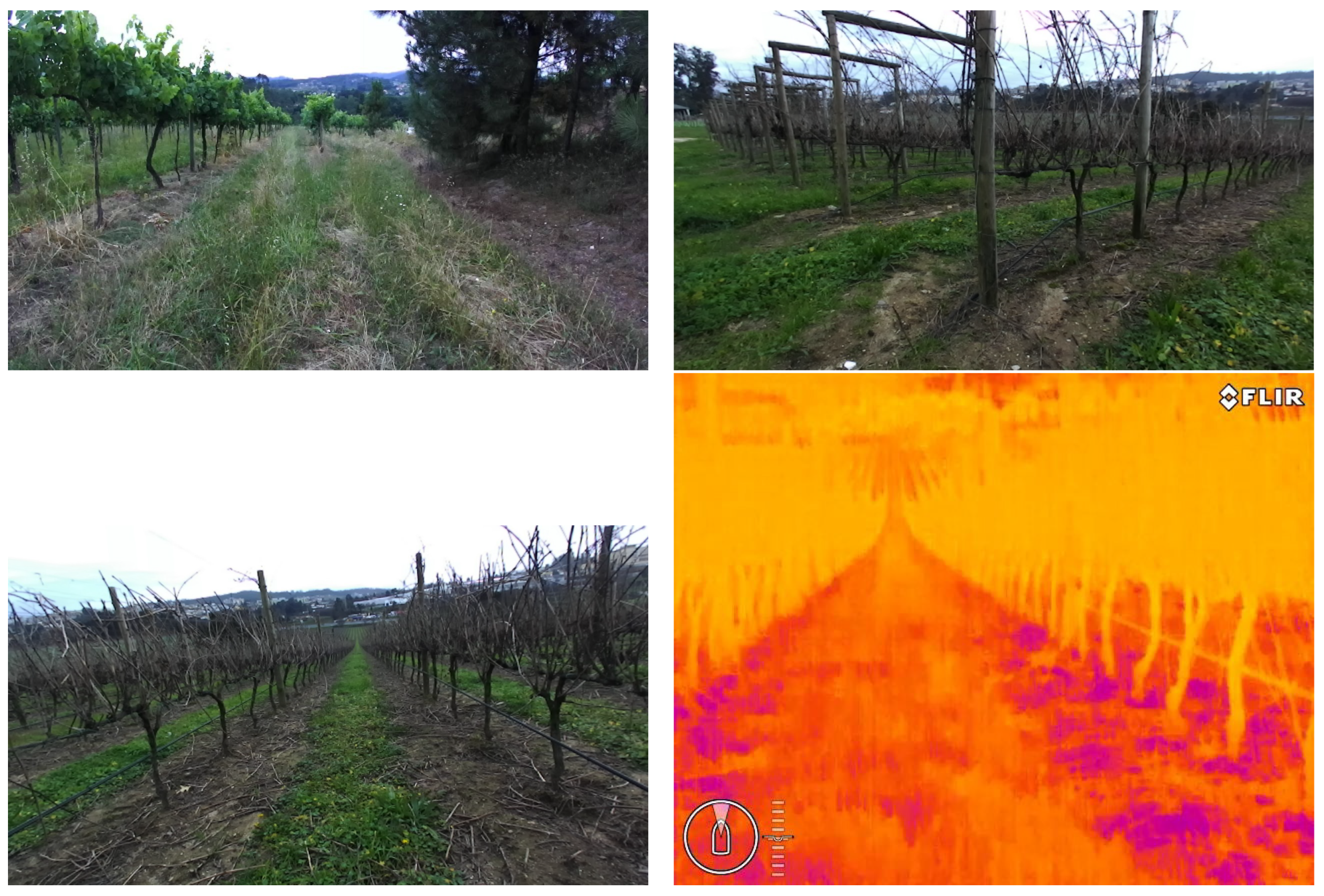
2.1. Dataset

The VineSet dataset from [26] was used for this work. Videos were captured from four different vineyards using a robot with a frontal stereo RGB camera and a frontal thermal camera [26]. Images were then extracted from the videos, resulting in a total of 952 vineyard images. The Vineset dataset contains a wide variety of data. The VineSet consists of images taken at different times of the year to capture the different characteristics of vineyards resulting from the temporal offset. In addition, it shows images of vineyards with and without vegetation and with different brightness levels. Finally, thermal images of vineyards are added to the dataset, introducing the concept of temperature, which can improve the learning process. A sample of the variety of images in the VineSet is shown in Figure 1.
In the next step, the images were manually labeled in the publicly available Pascal format VOC.
To increase the diversity and robustness of the VineSet, the augmentation methods were used in [26] and the images were expanded to 9481 images. For the following two reasons, the original data were used without augmentation:
  • The first and most important point was that the dataset was augmented before splitting the data into train and test. When performing the splits, the same image could appear in different splits with small changes in angle or brightness, which would have made the validation and testing step less effective (see Section 3.4).
  • Second, our computational power was limited. Training the DL models requires a system with very high computational power (GPU) and memory. The more input data, the more training time and the more memory required.

2.2. SSD Object Detection Model
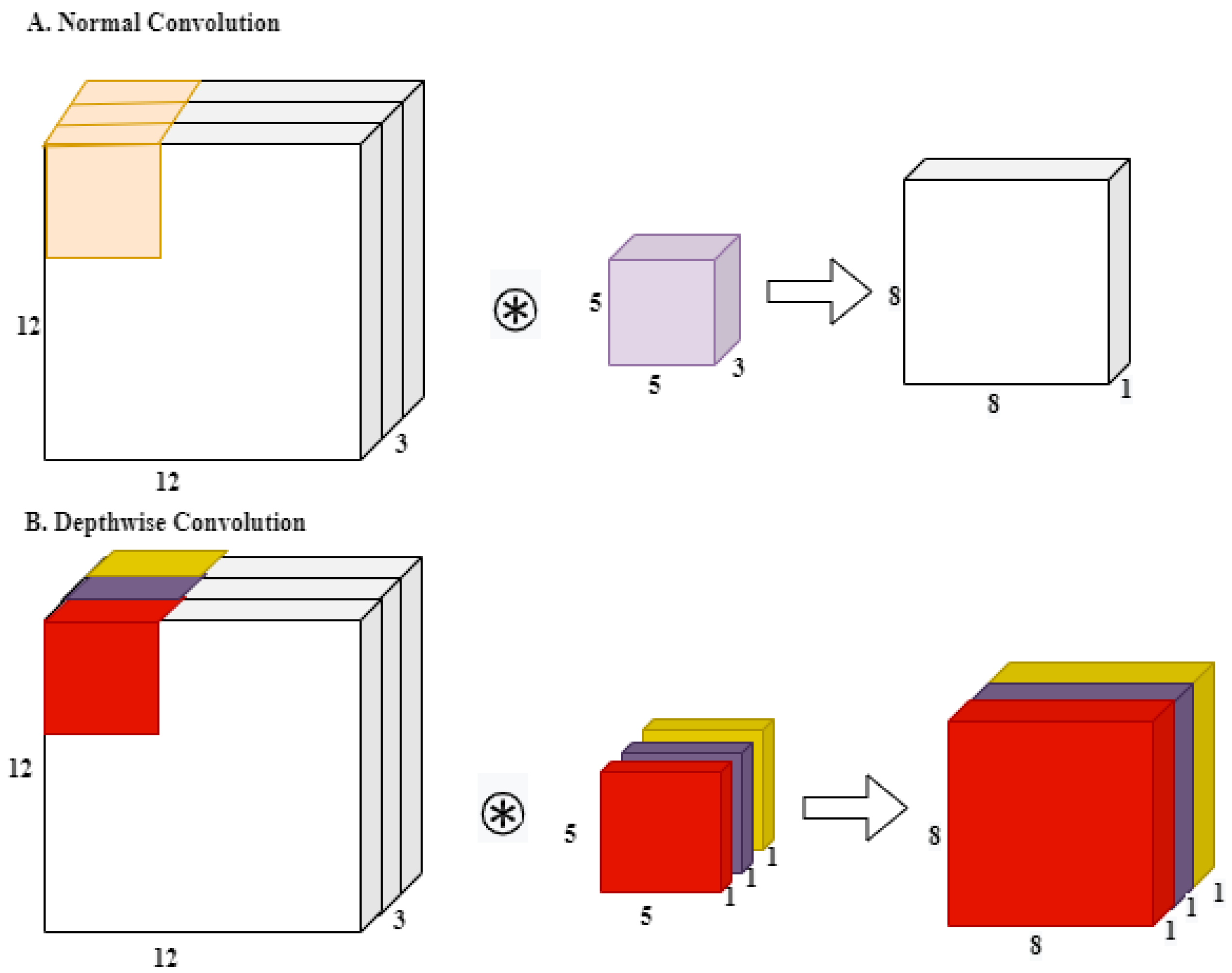
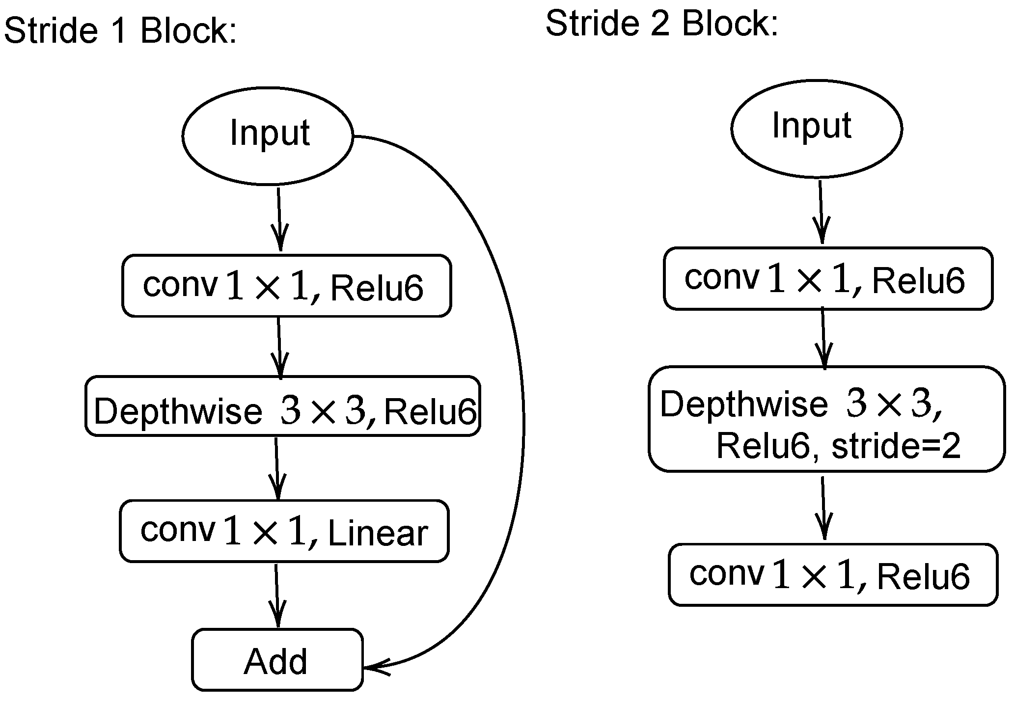
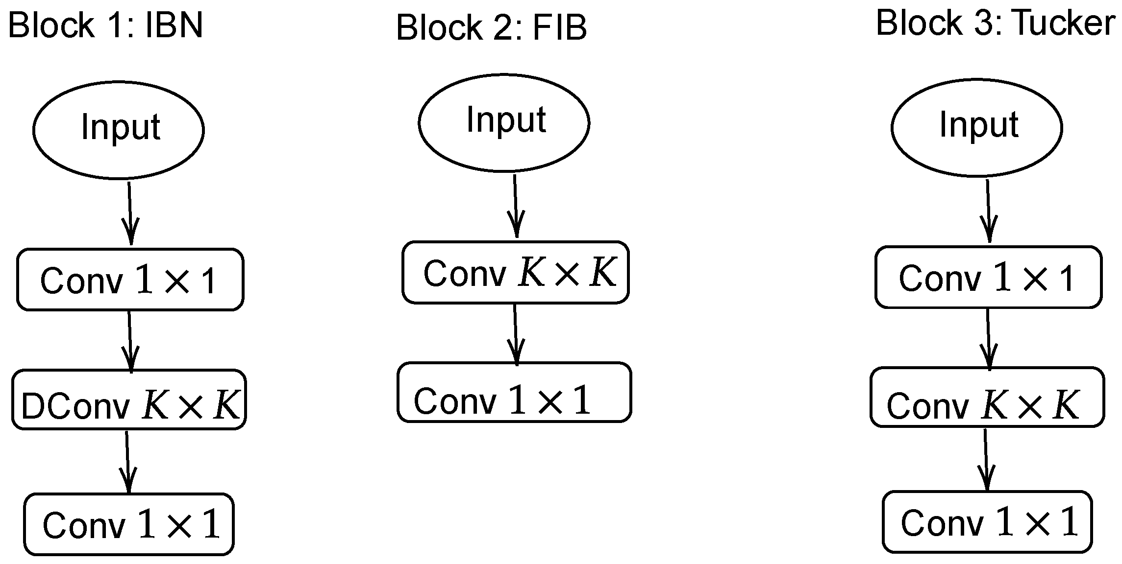
SSD consists of two components, a backbone model and an SSD head. The backbone is a classification model like the VGG-16 architecture without fully connected layers [22]. It is used to extract feature maps from the input image while preserving the spatial structure of the image. The head is a set of additional convolutional layers added to the backbone instead of the original fully connected layers [22]. The convolutional layers in the head are gradually reduced in size. In this way, features can be extracted at multiple scales, and the size of the input for each successive layer can be progressively reduced [22]. Figure 2 shows the SSD architecture with VGG as backbone.
Instead of using a sliding window, SSD splits the image using a grid and lets each grid cell be responsible for detecting objects in that area of the image. Each grid cell is capable of outputting the position and type of the object it contains. The anchor box and receptive field are designed to detect multiple objects or multiple objects of different shapes in a grid cell [22]. Using a 3 × 3 convolutional layer on the output of multiple layers, each grid cell (location) is assigned multiple bounding boxes (usually four or six boxes). These bounding boxes have different sizes and aspect ratios to cover objects of different sizes. For each of the bounding boxes, scores are calculated for each class, including an additional class for no object and 4 offsets, relative to the original shape of the default bounding box (see Figure 3). Essentially, the anchor box with the highest degree of overlap with an object is responsible for predicting the class and location of that object. The last layer is the non-maximum suppression layer to avoid detecting an object several times.
The SSD model is faster than the previous state of the art for single-stage detectors (YOLO) [27] and as accurate as Faster RCNN [22].

2.3. SSD Backbones

MobileNets are a tangled class of neural networks developed by Google researchers in 2017 [17]. These models are considered very useful for implementation on mobile and embedded devices. MobileNet uses depthwise separable convolutions. It significantly reduces the number of parameters compared to a network with regular convolutions with the same depth in the nets [17]. The main difference between normal convolutions and depth-wise convolutions is that in regular convolutions, the convolution operation is applied to all input channels, while in depth-wise convolutions, each channel remains separate [17] (see Figure 4). In MobileNet-V1, after applying a filter to each channel, a 1 × 1 convolutional layer is applied to combine the results of the depthwise convolution operation. Because depth-separable convolution requires less computation than regular convolution, MobileNets are faster and consume less power, so they can run on mobile and embedded devices without powerful graphics processors.
Due to the small size, there is a trade-off in accuracy compared to larger, fully convolutional architectures. MobileNet-V2 [18] was designed to improve the accuracy of the MobileNet-V1. In MobileNet-V2, there are two types of blocks. One is a residual block with a stride of one and the other is a block with a stride of two for reduction (see Figure 5). Adding residual blocks allows the network to access previous feature maps that were not changed in the convolutional block. Additionally, a linear layer was used in the last layer of the residual block to prevent nonlinearities from destroying too much information. The other difference with MobileNet-V1 is that a low-cost 1 × 1 convolutional layer was used at the beginning of the blocks to reduce the number of input channels. This way, the following 3 × 3 convolutional layer has much less parameters.
MobileNet Edge TPU [28] was developed for the Edge TPU in the Pixel 4, which is similar in architecture to the Edge TPU in the Coral product, but adapted to the requirements of Pixel 4’s main camera functions. To optimize the model accuracy and latency of the Edge TPU, the Neural Architecture Search (NAS) [29] and NetAdapt [30] algorithms were used to search for the model structure. NAS is a process that searches among all possible combinations of submodules that can be repeatedly assembled to obtain the entire model with the best possible accuracy. The NetAdapt algorithm works with the number of filters in each convolutional layer. To find the best structure for MobileNet Edge TPU in terms of accuracy and latency, the NAS and NetAdapt algorithms were used side by side. The result is a structure that has lower latency or higher accuracy at fixed latency than existing mobile models such as MobileNet-V2 and the minimalistic MobileNet-V3 [28].
MobileDet [20] is a new architecture for image classification models designed specifically for use on mobile accelerators such as DSP, Edge TPU, and so on. In MobileNet Edge TPU, the NAS algorithm was used to find the best architecture for the classification model, but in [20], a new backbone search space is proposed based on full convolutions for the SSD object detection model. Figure 6 shows the three blocks used to build the MobileDet model.

2.4. Hardware Used

Training was performed on a desktop computer PC with an Intel(R) Core(TM) i7-4790 CPU @ 3.60GHz, 16 GB RAM, and an NVIDIA RTX 2080 graphics card with 8 GB memory.
The Raspberry Pi 4 Model B is the latest addition to the popular Raspberry Pi line of single-board computers. Compared to the previous generation Raspberry Pi 3 Model B, it offers revolutionary advances in CPU speed, multimedia capabilities, memory, and connectivity. In this study, the model was inferred to Edge devices with a Raspberry Pi 4 Model B with 8 GB of memory.
Coral USB Accelerator is a USB add-on module that provides accelerated ML inference for existing systems. Coral USB Accelerator was used on the Raspberry Pi to investigate the performance of the model designed for Edge TPU devices. Figure 7 shows the Raspberry Pi 4 and the Coral USB Accelerator.

2.5. Metric for Evaluation

The SSD model for object detection was evaluated using mean average accuracy (mAP). The mAP calculates a score by comparing the ground truth bounding box to the detected box. The mAP score is determined by precision (P), recall (R), and intersection over union (IoU). Precision is calculated using Equation (1) and is the proportion of true detection by the model (TP) to total positive detection (true positives and false positives (FP).
P = TP TP + FP .
Recall measures the proportion of accurate positive predictions among all possible positive and false negative (FN) predictions, is calculated by Equation (2).
R = TP TP + FN .
The IoU calculates the overlap between the ground truth bounding box and the boxes predicted by the model. It is a number in the range between zero and one. The number 1 means that the ground truth box completely matches the predicted box and zero means that there is no overlap between the two boxes, and is calculated according to Equation (3).
IoU = area   of   overlap area   of   union .
The precision–recall curve is calculated by the trade-off between precision and recall values for different IoU thresholds. The average precision is defined by the area under the precision–recall curve, and the mAP is the average over the average precision for each predicted box.

2.6. Training Configuration

Building a DL model from scratch requires a large amount of data and computational resources. One way to get around this drawback is to use transfer learning and fine-tuning [11,26,31]. In transfer learning, the model is trained with a large dataset such as ImageNet or COCO, and then the same model is reused and re-trained for a similar task. The TensorFlow Model Garden is a repository of a number of different implementations of state-of-the-art models and modeling solutions for TensorFlow users [32]. The Object Detection directory of the Tensorflow Garden contains code implementations and pre-trained models from published research papers. These models have been trained on the COCO dataset and can be used for transfer learning and fine-tuning. In this work, the pre-trained models in the Tensorflow Garden were used for fine-tuning.
Normally, the default input of the models in the object detection directory is less than or equal to 320 × 320 . In this work, the model input of the model was changed to 640 × 480 to avoid degradation of the image and losing the information within the images. In Section 3.3, it is investigated that the size of the input makes a big difference in terms of the accuracy of the model and the time inference. Since the size of the input of the images was not mentioned in the [26], the SSD model was trained with mobiletV1 and mobiletV2 to compare the performance of the Edge TPU models.
Due to our limited computational power, the batch size of four was the best we could use to train the model. The models were trained with a maximum of 35,000 steps. The quantization-aware method was used. The quantization-aware method simulates low precision behavior in the forward pass while the backward pass remains the same [33]. The learning rate for each model was set to a range of 0.01 to 0.0455 and the IoU threshold was set to a range of 0.40 to 0.55 to obtain the best performance of the model for the dataset.

3. Results and Discussions

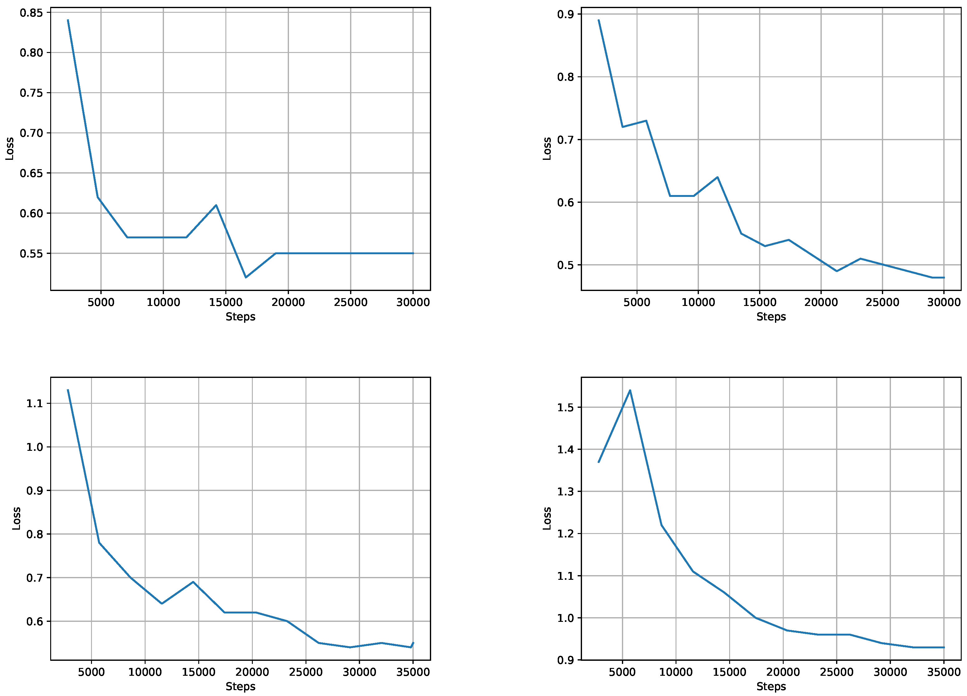
3.1. Performance of the Models during Training

Figure 8 and Figure 9 demonstrate the losses and mAP, respectively, of the models during training. As can be seen in Figure 8, the losses of MobileNet Edge TPU and MobileDet Edge TPU are more stable than those of the other two models. Furthermore, MobileDet Edge TPU performs better in terms of mAP on the test set at PC, although it has a larger overall loss than the other models at the end of training.
Since the mAP improvement of MobileNet-V1 and MobileNet-V2 ended at about 25k steps (Figure 9), their training was terminated at 30k steps, whereas the other models were trained for 35k steps.
Table 1 shows the training time (s) of the models per step. The training time of the models developed for the Edge TPU was shorter than that of the other models, which is due to the fact that the number of parameters of these models is less than that of the other two models. Although the SSD with MobileNet Edge TPU and MobileDet Edge TPU have fewer parameters, their performance is superior to the other two types (see Figure 9).

3.2. Comparison of the Performance of the Models

An illustration of detection using SSD MobileDet Edge TPU is shown in Figure 10. The detection using the model is shown on the left, while the ground truth is shown on the right. As we can see, the model was able to identify a tree trunk in the image, despite its distance from the camera and its modest size.
Table 2 shows the performance of the SSD model with different models as backbones on the GPU and the Raspberry Pi. From the table, it can be seen that the best performance in terms of accuracy on PC was achieved by the SSD model with MobileDet Edge TPU and on the RaspberryPi with MobileNet Edge TPU. The degradation in accuracy when switching from a PC to a Raspberry Pi was less with the MobileNet Edge TPU than with the other models. Although the SSD with MobileNet-V2 model and the MobileDet model performed better than SSD with MobileNet Edge TPU on PC, the accuracy on the RaspberryPi decreases. MobileNet-V1 achieved the worst results on PC and the Raspberry Pi.
It is interesting to note that for all models, the accuracy of the model running on the Raspberry Pi with TPU is superior to the accuracy of the model running on the Raspberry Pi without TPU.
On the Raspberry Pi with TPU, the models all have virtually the same inference time, with the SSD achieving the fastest inference time with MobileNet-V1 as the backbone.
The inference time for the models created for the TPU is longer than MobileNet-V1 and V2 on the RaspberryPi without TPU, but it is the same on the RaspberryPi with TPU.
Figure 11 shows the mean average accuracy versus latency of the trained models on the RaspberryPi without and with TPU. As can be seen, the models created for the TPU perform better on the TPU, however the inference time is longer than MobileNet-V1. Depending on the application, the model should be chosen because there is a trade-off between accuracy and latency.

3.3. Effect of Some Parameters on the Performance of the Model

To investigate the effect of input image size on the performance of the model, the SSD was trained using MobileDet as the backbone with the default input size, i.e., 320 × 320 . The performance of the model is shown in Table 3. As can be seen from the table, the accuracy of the model decreases by 12%, and the time for inference decreases by almost half. Thus, there is a trade-off between the input size of the model, the accuracy and time for inference. A model with a smaller input size is less accurate, but runs faster.
In the following experiment, 20% of the training dataset was used for training to investigate the effect of dataset size on model performance. The SSD with MobileDet as the backbone was trained on this smaller dataset with the same hyperparameters as the model with the best performance. As can be seen in Table 3, the performance of the model drops by 8%.
The thermal images in the training dataset were removed from the training to examine the effect of having thermal images in the training set. The performance of the model dropped by 2%.
The images of trunks without leaves were selected as the training set (304 images) for the next experiment, and the images of trunks with leaves were selected as the validation set (89 images). Figure 12 shows the performance of the model during the training of the model on the validation set. The model was trained in 17,500 steps with an mAP of less than 0.05, while the model trained with the mixed images (with and without leaves) almost reached an mAP of 0.8 in the same step (see Figure 9). Therefore, the training set must fully reflect the real-world conditions, otherwise, the model will not be able to detect the desired object in the unseen images, which contain features not seen during training. It is important to note that the model could not detect trunks with leaves when trained on images without leaves, however adding some images with leaves (89 images) enhanced the performance of the model. Consequently, updating and re-training the model with new data obtained in the field is an important step in training and using the DL algorithms.

3.4. Effect of Data Augmentation before Splitting Data into Training and Test Set

As mentioned in Section 2.1, enhancing images prior to splitting the data into training and test data results in certain images to appear in different partitions with slight variations in brightness or angle, which reduces the effectiveness of validation and testing. To investigate this further, a random image was selected and image enhancements such as rotation (15 and 45 degrees) and flipping of this image were added to the training dataset. Figure 13 shows the result of the model with and without adding an enhanced version of the image and ground truth. As can be seen in Figure 13, the trained model with enhanced copies of the image as part of the training dataset produces identical results to the ground truth, but the model can identify even more trunks on the image when the enhanced versions are not used in the training. Consequently, either the process of data augmentation should be performed after splitting the dataset into a training and a test dataset, or care should be taken to ensure that an enhanced version of the image from the test dataset is not used in the training dataset.

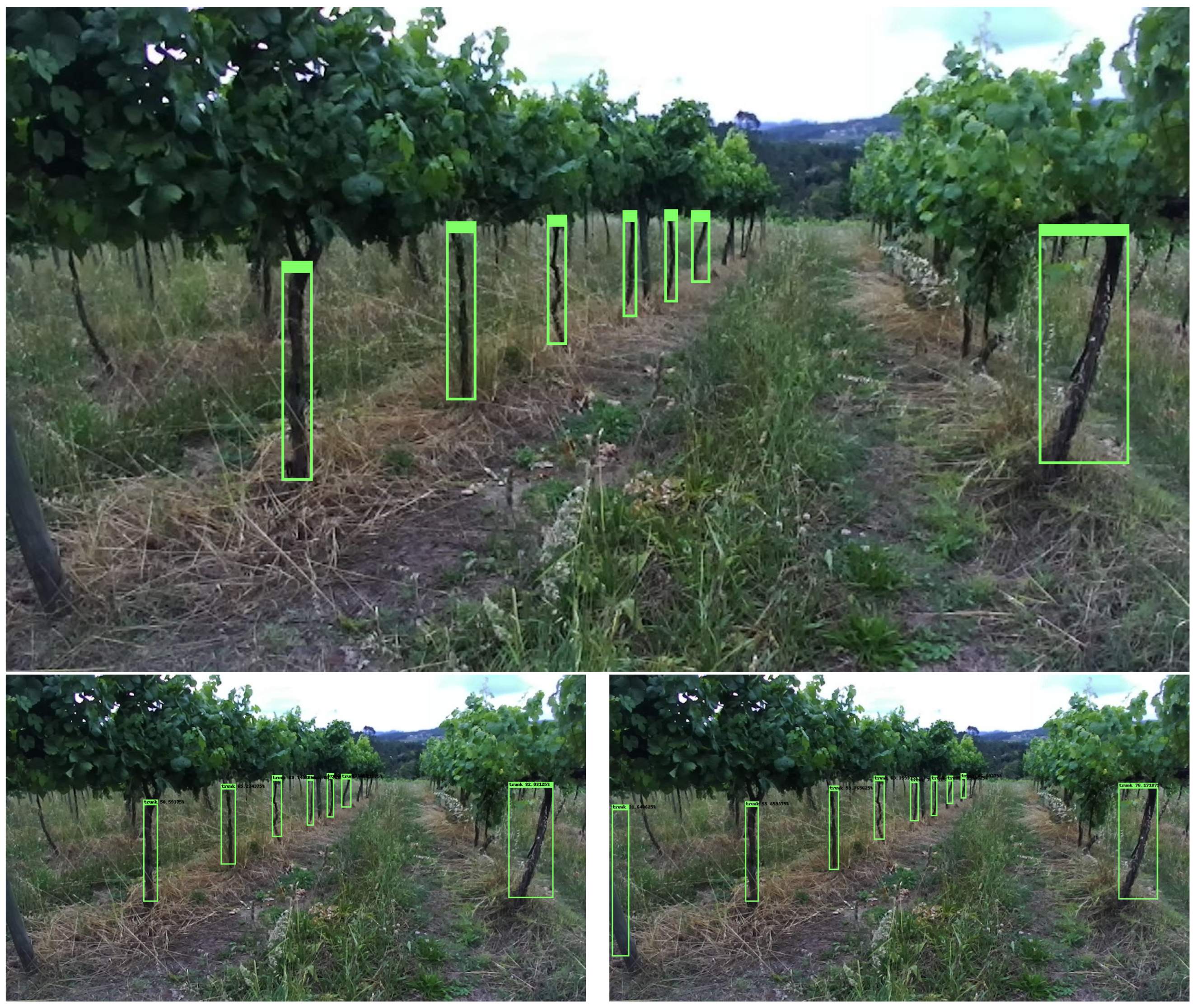
3.5. Analysis of the Trunk Detection Results

In analyzing the model results in detecting tree trunks, we found some cases where a tree trunk is not marked in the ground truth, but the model can still find it in the images. Figure 14 shows an example of this case.
When the trunks are close together, as is the case in some images, the model cannot detect both of them. This situation is illustrated in Figure 15. Since the overlap occurs while the trunks are far from the camera and the robots are moving through the field, the overlap of the trunks in the close-up image is minimal and therefore does not pose a problem for the robot application. However, more photos with overlapping trunks should be added to the training dataset, and the model should be re-trained to reduce the error in detecting the overlapping trunks.
When the surroundings are extremely complicated and the trunks are far from the camera, the model also has difficulty accurately identifying all the trunks in the image. Examples of this case are shown in Figure 16. As can be seen, the environment is quite complex because the trunks are far from the camera and there are plants in the middle of the row, making it difficult for the model to identify all the stems in the image.

4. Conclusions

In this study, the two state-of-the-art object detection models for use on TPU devices were trained to detect the tree trunk in a vineyard. The best performance on PC in terms of accuracy was achieved by the SSD with MobileDet Edge TPU model compared to the SSD with MobileNet Edge TPU, MobileNet-V1, and MobileNet-V2. However, the degradation of the accuracy of MobileNet Edge TPU was less when the model was transferred to the RaspberryPi with TPU and performed the best on this device. Therefore, the accuracy of the model should be measured on the edge devices to ensure the performance of the model on these devices.
This work also examined the relationship between input size and accuracy and inference time on edge devices. By changing the model input from 320 × 320 to 640 × 480 , the accuracy and inference time increased simultaneously. Therefore, the model input size should be considered as a trade-off factor for training the model.
In addition, this work investigated how the size of the training dataset and the number of thermal images in the training dataset affect the detection results. When the size of the training dataset was reduced to 20%, the performance of the model decreased by 8%, and when thermal images were excluded from the training set, the performance of the model decreased by 2%.
The analysis of the detection of the model on the test set shows that the wrong labeling, the complex environment, the fused trunk, or the trunk far away from the camera can lead to false detection of the model.
The limitation of DL models is that the output of the trained model depends on the training dataset. According to this work, a model trained on images without leaves is often unable to detect a tree trunk with leaves. To avoid this drawback, the training model data should be collected at different seasons and under real conditions. When using DL models, updating and re-training the model with new data collected in the field should also be considered an important step. The fact that the models from DL require a large amount of training data is another drawback that makes it difficult to use these models in agriculture. However, sharing the dataset in research projects such as VineSet helps to advance the research field.

Author Contributions

K.A.: investigation; methodology; writing—review, software. E.A.: methodology; software. P.D.G.: supervision, writing review, and project administration and Funding acquisition. V.N.G.J.S.: funding acquisition, reviewing and editing. J.M.L.P.C.: funding acquisition, reviewing and editing. All authors have read and agreed to the published version of the manuscript.

Funding

This research received no external funding.

Data Availability Statement

Not applicable, the study does not report any data.

Acknowledgments

K.A. and P.D.G. acknowledge the R&D Project BioDAgro–Sistema operacional inteligente de informação e suporte á decisão em AgroBiodiversidade, project PD20-00011, promoted by Fundação La Caixa and Fundação para a Ciência e a Tecnologia, taking place at the C-MAST-Centre for Mechanical and Aerospace Sciences and Technology, Department of Electromechanical Engineering of the University of Beira Interior, Covilhã, Portugal. P.D.G. and E.A. acknowledges the PrunusBot project—Autonomous controlled spraying aerial robotic system and fruit production forecast, Operation No. PDR2020-101-031358 (leader), Consortium No. 340, Initiative No. 140, promoted by PDR2020 and co-financed by the EAFRD and the European Union under the Portugal 2020 program. P.D.G. also acknowledges Fundação para a Ciência e a Tecnologia (FCT—MCTES) for its financial support via project UIDB/00151/2020 (C-MAST). V.N.G.J.S. and J.M.L.P.C. acknowledge that this work is funded by FCT/MCTES through national funds and, when applicable, co-funded EU funds under project UIDB/EEA/50008/2020.

Conflicts of Interest

The authors declare no conflict of interest.

References

  1. Clark, M.; Tilman, D. Comparative analysis of environmental impacts of agricultural production systems, agricultural input efficiency, and food choice. Environ. Res. Lett. 2017, 12, 064016. [Google Scholar] [CrossRef]
  2. Baiano, A. An Overview on Sustainability in the Wine Production Chain. Beverages 2021, 7, 15. [Google Scholar] [CrossRef]
  3. Rodrigo-Comino, J. Five decades of soil erosion research in “terroir”. The State-of-the-Art. Earth-Sci. Rev. 2018, 179, 436–447. [Google Scholar] [CrossRef]
  4. Jastrzębska, M.; Kostrzewska, M.; Saeid, A. Chapter 2—Sustainable agriculture: A challenge for the future. In Smart Agrochemicals for Sustainable Agriculture; Chojnacka, K., Saeid, A., Eds.; Academic Press: Cambridge, MA, USA, 2022; pp. 29–56. [Google Scholar] [CrossRef]
  5. Hopmans, J.W.; Qureshi, A.; Kisekka, I.; Munns, R.; Grattan, S.; Rengasamy, P.; Ben-Gal, A.; Assouline, S.; Javaux, M.; Minhas, P.; et al. Chapter One—Critical knowledge gaps and research priorities in global soil salinity. In Advances in Agronomy; Academic Press: Cambridge, MA, USA, 2021; Volume 169, pp. 1–191. [Google Scholar] [CrossRef]
  6. Nalla, K.; Pothabathula, S.V.; Kumar, S. Chapter 21—Applications of Computational Methods in Plant Pathology. In Natural Remedies for Pest, Disease and Weed Control; Egbuna, C., Sawicka, B., Eds.; Academic Press: Cambridge, MA, USA, 2020; pp. 243–250. [Google Scholar] [CrossRef]
  7. Loures, L.; Chamizo, A.; Ferreira, P.; Loures, A.; Castanho, R.; Panagopoulos, T. Assessing the Effectiveness of Precision Agriculture Management Systems in Mediterranean Small Farms. Sustainability 2020, 12, 3765. [Google Scholar] [CrossRef]
  8. Verdouw, C.; Wolfert, S.; Tekinerdogan, B. Internet of Things in agriculture. CAB Rev. 2016, 11, 1–12. [Google Scholar] [CrossRef]
  9. Zantalis, F.; Koulouras, G.; Karabetsos, S.; Kandris, D. A Review of Machine Learning and IoT in Smart Transportation. Future Internet 2019, 11, 94. [Google Scholar] [CrossRef] [Green Version]
  10. Kamilaris, A.; Prenafeta-Boldú, F.X. Deep learning in agriculture: A survey. Comput. Electron. Agric. 2018, 147, 70–90. [Google Scholar] [CrossRef] [Green Version]
  11. Alibabaei, K.; Gaspar, P.D.; Lima, T.M.; Campos, R.M.; Girão, I.; Monteiro, J.; Lopes, C.M. A Review of the Challenges of Using Deep Learning Algorithms to Support Decision-Making in Agricultural Activities. Remote Sens. 2022, 14, 638. [Google Scholar] [CrossRef]
  12. Kerkech, M.; Hafiane, A.; Canals, R. Vine disease detection in UAV multispectral images using optimized image registration and deep learning segmentation approach. Comput. Electron. Agric. 2020, 174, 105446. [Google Scholar] [CrossRef]
  13. Silver, D.L.; Monga, T. In Vino Veritas: Estimating Vineyard Grape Yield from Images Using Deep Learning. In Advances in Artificial Intelligence; Meurs, M.J., Rudzicz, F., Eds.; Springer International Publishing: Cham, Switzerland, 2019; pp. 212–224. [Google Scholar]
  14. Ghiani, L.; Sassu, A.; Palumbo, F.; Mercenaro, L.; Gambella, F. In-Field Automatic Detection of Grape Bunches under a Totally Uncontrolled Environment. Sensors 2021, 21, 3908. [Google Scholar] [CrossRef]
  15. Milella, A.; Marani, R.; Petitti, A.; Reina, G. In-field high throughput grapevine phenotyping with a consumer-grade depth camera. Comput. Electron. Agric. 2019, 156, 293–306. [Google Scholar] [CrossRef]
  16. Majeed, Y.; Karkee, M.; Zhang, Q.; Fu, L.; Whiting, M.D. Determining grapevine cordon shape for automated green shoot thinning using semantic segmentation-based deep learning networks. Comput. Electron. Agric. 2020, 171, 105308. [Google Scholar] [CrossRef]
  17. Howard, A.G.; Zhu, M.; Chen, B.; Kalenichenko, D.; Wang, W.; Weyand, T.; Andreetto, M.; Adam, H. MobileNets: Efficient Convolutional Neural Networks for Mobile Vision Applications. arXiv 2017, arXiv:1704.04861. [Google Scholar]
  18. Sandler, M.; Howard, A.; Zhu, M.; Zhmoginov, A.; Chen, L.C. MobileNetV2: Inverted Residuals and Linear Bottlenecks. arXiv 2018, arXiv:1801.04381. [Google Scholar]
  19. Howard, A.; Sandler, M.; Chu, G.; Chen, L.C.; Chen, B.; Tan, M.; Wang, W.; Zhu, Y.; Pang, R.; Vasudevan, V.; et al. Searching for MobileNetV3. arXiv 2019, arXiv:cs.CV/1905.02244. [Google Scholar]
  20. Xiong, Y.; Liu, H.; Gupta, S.; Akin, B.; Bender, G.; Wang, Y.; Kindermans, P.J.; Tan, M.; Singh, V.; Chen, B. MobileDets: Searching for Object Detection Architectures for Mobile Accelerators. arXiv 2021, arXiv:cs.CV/2004.14525. [Google Scholar]
  21. Cloud Tensor Processing Units (tpus). Available online: https://cloud.google.com/tpu/docs/tpus (accessed on 27 June 2022).
  22. Liu, W.; Anguelov, D.; Erhan, D.; Szegedy, C.; Reed, S.; Fu, C.Y.; Berg, A.C. SSD: Single Shot MultiBox Detector. In Computer Vision-ECCV 2016; Springer International Publishing: Cham, Switzerland, 2016; pp. 21–37. [Google Scholar]
  23. Aguiar, A.S.; Magalhães, S.A.; dos Santos, F.N.; Castro, L.; Pinho, T.; Valente, J.; Martins, R.; Boaventura-Cunha, J. Grape Bunch Detection at Different Growth Stages Using Deep Learning Quantized Models. Agronomy 2021, 11, 1890. [Google Scholar] [CrossRef]
  24. Aghi, D.; Mazzia, V.; Chiaberge, M. Local Motion Planner for Autonomous Navigation in Vineyards with a RGB-D Camera-Based Algorithm and Deep Learning Synergy. Machines 2020, 8, 27. [Google Scholar] [CrossRef]
  25. Pinto de Aguiar, A.S.; Neves dos Santos, F.B.; Feliz dos Santos, L.C.; de Jesus Filipe, V.M.; Miranda de Sousa, A.J. Vineyard trunk detection using deep learning—An experimental device benchmark. Comput. Electron. Agric. 2020, 175, 105535. [Google Scholar] [CrossRef]
  26. Aguiar, A.S.; Monteiro, N.N.; Santos, F.N.D.; Solteiro Pires, E.J.; Silva, D.; Sousa, A.J.; Boaventura-Cunha, J. Bringing Semantics to the Vineyard: An Approach on Deep Learning-Based Vine Trunk Detection. Agriculture 2021, 11, 131. [Google Scholar] [CrossRef]
  27. Redmon, J.; Farhadi, A. YOLO9000: Better, Faster, Stronger. In Proceedings of the 2017 IEEE Conference on Computer Vision and Pattern Recognition (CVPR), Honolulu, HI, USA, 21–26 July 2017; pp. 6517–6525. [Google Scholar] [CrossRef] [Green Version]
  28. Yazdanbakhsh, A.; Seshadri, K.; Akin, B.; Laudon, J.; Narayanaswami, R. An Evaluation of Edge TPU Accelerators for Convolutional Neural Networks. arXiv 2021, arXiv:cs.LG/2102.10423. [Google Scholar]
  29. Zoph, B.; Le, Q.V. Neural Architecture Search with Reinforcement Learning. arXiv 2016, arXiv:1611.01578. [Google Scholar]
  30. Yang, T.J.; Howard, A.; Chen, B.; Zhang, X.; Go, A.; Sandler, M.; Sze, V.; Adam, H. NetAdapt: Platform-Aware Neural Network Adaptation for Mobile Applications. arXiv 2018, arXiv:cs.CV/1804.03230. [Google Scholar]
  31. Pan, S.J.; Yang, Q. A Survey on Transfer Learning. IEEE Trans. Knowl. Data Eng. 2010, 22, 1345–1359. [Google Scholar] [CrossRef]
  32. Yu, H.; Chen, C.; Du, X.; Li, Y.; Rashwan, A.; Hou, L.; Jin, P.; Yang, F.; Liu, F.; Kim, J.; et al. TensorFlow Model Garden. Available online: https://github.com/tensorflow/models (accessed on 27 June 2022).
  33. Nagel, M.; Fournarakis, M.; Amjad, R.A.; Bondarenko, Y.; van Baalen, M.; Blankevoort, T. A White Paper on Neural Network Quantization. arXiv 2021, arXiv:2106.08295. [Google Scholar]
Figure 1. An example of the variety of images in the database.
Futureinternet 14 00199 g001
Figure 2. SSD architecture.
Futureinternet 14 00199 g002
Figure 3. 8 × 8 Feature Map with 4 default boxes at position ( 3 , 3 ) . For each of the boxes, four offsets and class values are predicted for p classes.
Futureinternet 14 00199 g003
Figure 4. (A) shows a normal convolution with 8 × 8 × 1 output and (B) shows a depthwise convolution with three kernels to get an image with 8 × 8 × 3 image.
Futureinternet 14 00199 g004
Figure 5. Blocks used in MobileNet-V2.
Futureinternet 14 00199 g005
Figure 6. Blocks used in MobileDet.
Futureinternet 14 00199 g006
Figure 7. From left to right: Raspberrypi (https://www.raspberrypi.com/, accessed on 15 November 2021), and Google coral USB Accelerator (https://coral.ai/, accessed on 8 November 2021).
Futureinternet 14 00199 g007
Figure 8. Loss of models during training. Top left: MobileNet-V1, top right: MobileNet-V2, bottom left: MobileNet Edge TPU and bottom right: MobileDet Edge TPU.
Futureinternet 14 00199 g008
Figure 9. mAP of models during training (threshold = 50). Top left: MobileNet-V1, top right: MobileNet-V2, bottom left: MobileNet Edge TPU and bottom right: MobileDet Edge TPU.
Futureinternet 14 00199 g009
Figure 10. Detection results using SSD MobileDet Edge TPU.
Futureinternet 14 00199 g010
Figure 11. Comparison of mean average precision vs. latency for mobile models.
Futureinternet 14 00199 g011
Figure 12. mAP of the SSD MobileDet model, trained on the images without leaves and tested on the images with leaves.
Futureinternet 14 00199 g012
Figure 13. Detection results of the trained models with and without enhanced images in the training dataset. Top image: ground truth, bottom left: Model trained with enhanced images, bottom right: Model trained without enhanced images.
Futureinternet 14 00199 g013
Figure 14. The left images are the detection results of the model, and the left side is the ground truth. The model has found the trunks in the image that are not marked as tree trunks.
Futureinternet 14 00199 g014
Figure 15. Two trunks are close together and the model cannot detect both.
Futureinternet 14 00199 g015
Figure 16. The result of the model in the complex environment.
Futureinternet 14 00199 g016
Table 1. The total number of parameters and the training duration for one step.
BackbonesMobileNet-V1MobileNet-V2MobileNet
Edge TPU
MobileDet
Edge TPU
Training time (s)0.230.300.190.19
No. Parameters (million)5.494.572.993.25
Table 2. Performance of the models in terms of accuracy and inference time (ms).
BackbonemAP%Inference Time (ms)
PCRaspberryPiRaspberryPi
GPUCPUTPUCPUTPU
MobileDet Edge TPU8984.484.61048.27747.75
MobileNet Edge TPU86.784.886.61235.7347.79
MobileNet-V18479.981.3861.445.73
MobileNet-V28882.883.2773.71747.969
Table 3. Performance of the SSD MobileDet under different parameters.
BackbonemAP%Inference Time (ms)
PCRaspberryPiRaspberryPi
GPUCPUTPUCPUTPU
MobileDet Edge TPU ( 640 × 480 )8984.484.6456.9847.75
MobileDet Edge TPU ( 320 × 320 )7767.4671235.7327
MobileDet Edge TPU ( 640 × 480 )817777.5456.9847.75
(trained on 20% of images)
MobileDet Edge TPU ( 640 × 480 )8782.683456.9847.75
(without thermal images in training set)
Publisher’s Note: MDPI stays neutral with regard to jurisdictional claims in published maps and institutional affiliations.

