Article

TQU-SLAM Benchmark Dataset for Comparative Study to Build Visual Odometry Based on Extracted Features from Feature Descriptors and Deep Learning

1
Faculty of Engineering Technology, Hung Vuong University, Viet Tri City 35100, Vietnam
2
Faculty of Basic Science, Tan Trao University, Tuyen Quang City 22000, Vietnam
*
Author to whom correspondence should be addressed.
Future Internet 2024, 16(5), 174; https://doi.org/10.3390/fi16050174
Submission received: 24 April 2024 / Revised: 7 May 2024 / Accepted: 15 May 2024 / Published: 17 May 2024
(This article belongs to the Special Issue Machine Learning Techniques for Computer Vision)

Abstract

:
The problem of data enrichment to train visual SLAM and VO construction models using deep learning (DL) is an urgent problem today in computer vision. DL requires a large amount of data to train a model, and more data with many different contextual and conditional conditions will create a more accurate visual SLAM and VO construction model. In this paper, we introduce the TQU-SLAM benchmark dataset, which includes 160,631 RGB-D frame pairs. It was collected from the corridors of three interconnected buildings comprising a length of about 230 m. The ground-truth data of the TQU-SLAM benchmark dataset were prepared manually, including 6-DOF camera poses, 3D point cloud data, intrinsic parameters, and the transformation matrix between the camera coordinate system and the real world. We also tested the TQU-SLAM benchmark dataset using the PySLAM framework with traditional features such as SHI_TOMASI, SIFT, SURF, ORB, ORB2, AKAZE, KAZE, and BRISK and features extracted from DL such as VGG, DPVO, and TartanVO. The camera pose estimation results are evaluated, and we show that the ORB2 features have the best results ( E r r d = 5.74 mm), while the ratio of the number of frames with detected keypoints of the SHI_TOMASI feature is the best ( r d = 98.97 % ). At the same time, we also present and analyze the challenges of the TQU-SLAM benchmark dataset for building visual SLAM and VO systems.

1. Introduction

Visual odometry (VO) is applied in many fields, such as [1] autonomous vehicles, unmanned aerial vehicles, underwater robots, space exploration robots, agriculture robots, medical robots, and AR/VR. Therefore, VO has been of research interest for many years. Based on the research of Neyestani et al. [2], Agostinho et al. [3], and Wang et al. [1], the problem of estimating VO using a vision-based method with monocular camera data is solved using two methods: knowledge-based and learning-based methods. Learning-based methods are based on traditional machine learning and DL. Knowledge-based methods include appearance-based methods, feature-based methods, and hybrid methods. Image-based VO is the process of determining the position and orientation of a robot or entity by analyzing a set of images obtained from its environment. As in the Neyestani et al. [2] study, the framework to build a VO system includes five steps, with input data being images, feature detection, feature tracking, motion estimation, triangulation, and trajectory estimation, as shown in Figure 1. The output of the VO framework is 6-DOF including 3D pose, which is the position of the camera in the scene; the remaining 3D information comprises the direction of camera movement.
Based on feature-based methods, the feature-detection step comprises the process of feature extraction, such as SIFT [4], SURF [5], ORB [6], and BRISK [7] features, etc. Detected features are tracked on consecutive frames to find the corresponding points on the frames using techniques such as optical flow [8]. This is followed by a motion-estimation step that typically uses epipolar geometry constraints to incorporate feature-to-feature matching (2D to 2D). From there, motion parameters are calculated, and projection from 3D to 2D is performed to minimize 3D tracked landmarks against the current image frame, and 3D to 3D is incorporated to increase the accuracy of the estimated pose. To perform camera pose optimization, research often uses algorithms such as Bundle adjustment, Kalman Filter, and EKF Graph optimization [1]. For DL-based methods, the steps of feature detection, feature matching, and pose estimation are performed using DL [1].
Currently, most VO estimation methods are evaluated on the KITTI dataset [9,10,11], TUM RGB-D SLAM dataset [12], NYUDepth dataset [13], and ICL-NUIM dataset [14]. However, DL methods always need a very large amount of data to train a VO estimation model. With this approach, the more data that are trained, and trained in more contexts, the more accurate the VO estimation results will be. In this paper, we propose a standard dataset called the TQU-SLAM benchmark dataset to evaluate VO estimation methods. Our dataset was collected using an Intel RealSense D435 in an environment comprising the second floor of three interconnected buildings: Building A, Building B, and Building C. This dataset includes 160,631 RGB-D frame pairs. The data were collected over a particular length (FO-D is 230.63 m, OP-D is 228.13 m) and were collected four times and eight times.
To see the challenges in the TQU-SLAM benchmark dataset, we tested the proposed dataset using PySLAM [15], with traditional features extracted at the feature-extraction step by feature descriptors, such as ORB [16], ORB2 [17], SIFT [4], SURF [5], BRISK [7], AKAZE [18], and KAZE [18], or features extracted from a DL model such as VGG [19], DPVO [20], and TartanVO [21]. In this paper, we perform VO construction on the entire TQU-SLAM benchmark dataset.
Our paper has the following main contributions:
  • We introduce the TQU-SLAM benchmark dataset for evaluating VO models, algorithms, and methods. The ground truth of the TQU-SLAM benchmark dataset is constructed by hand, including the camera coordinates in the real-world coordinate system, 3D point cloud data, intrinsic parameters, and the transformation matrix between the camera coordinate system and the real world.
  • We experiment with the TQU-SLAM benchmark dataset for estimating VO based on PySLAM [15,22] with the features extracted such as ORB [16], ORB2 [17], SIFT [4], SURF [5], BRISK [7], AKAZE [18], and KAZE [18], or features extracted from a DL model such as VGG [19], DPVO [20], and TartanVO [21].
  • The results are analyzed and compared with the TQU-SLAM benchmark dataset with many types of traditional features and features extracted from DL models.
The structure of our paper is organized as follows: Related studies are presented in Section 2. Section 3 introduces the TQU-SLAM benchmark dataset and the process of building ground-truth data of the camera’s moving trajectory. Section 4 presents the testing of the TQU-SLAM benchmark dataset with traditional features and features extracted from DL. The experiments, results, and challenges of VO estimation of the TQU-SLAM benchmark dataset are shown in Section 5. Finally, conclusions and future research are presented in Section 6.

2. Related Works

The VO process was also presented in great detail in the survey studies of Agostinho et al. [3], Neyestani et al. [2], and He et al. [23]. In this section, we present two problem areas: VO methods, VO models, and VO algorithms; and datasets to evaluate VO models and VO techniques.
About the research on VO methods, Agostinho et al. [3] built a taxonomy that includes two approaches to building VO: knowledge-based methods and learning-based methods. Knowledge-based methods include the following techniques, as illustrated in Figure 2: appearance-based techniques, feature-based techniques, and hybrid techniques. Learning-based methods include traditional machine learning techniques and deep learning techniques.
In research on knowledge-based methods, Davison et al. [24] proposed an algorithm called MonoSLAM to construct real-time 3D motion trajectories from data acquired from a camera. MonoSLAM can perform localization and mapping at a speed of 30 Hz on a computer with normal configuration. In particular, the structure-from-motion algorithm is used so that MonoSLAM can work on longer frame sequences. Klein et al. [25] proposed the PTAM technique to perform camera poses in an unexplored scene. The PTAM technique is used to perform two tasks, tracking the camera’s position and performing environmental mapping, with two parallel streams; of these, the mapping task is performed based on keyframes using the bundle adjustment technique. New points are initialized using an epipolar search. Ganai et al. [26] proposed a DTAM system that can perform real-time tracking and reconstruction of camera positions with high parallelization capabilities. This system does not use feature extraction but rather uses the density of pixels, identifying a patchwork surface with built-in keyframes by estimating depth. Izadi et al. [27] proposed the KinectFusion system, which allows building 3D pose Kinect cameras/depth cameras, with many tasks performed in parallel using GPU: 3D reconstruction using CAD models, the creation of models that are geometrically precise based on built point cloud data, and the creation of 3D models using mesh representation. Kerl et al. [28] proposed the DVO and LSD-SLAM system to build a visual SLAM system based on dense RGB-D images. The authors are used to extend the geometry method to include a geometric error term and perform frame-to-frame matching. The pose graph has a new keyframe inserted when one is detected. At the same time, an entropy-based technique is used to detect loop closure for eliminating drift. Forster et al. [29] proposed an SVO system to build a fast, accurate VO from a camera’s data. This method performs semi-directly and thus can reduce feature extraction and enhance matching techniques for motion estimation. To estimate camera pose and scene structure, SVO is divided into two classes: feature-based methods that use epipolar geometry to estimate camera motion and image structure, and methods that use invariant feature descriptors to estimate the scene from the combination of consecutive frames. The second type are direct methods, where intensity values are used to directly estimate the structure and movement of the camera. Bloesch et al. [30,31] proposed ROVIO to track and estimate camera positions using pixel-intensity errors of image patches. Then, the extended Kalman filter algorithm is used to monitor multilevel patch features. Whelan et al. [32,33] proposed a visual SLAM system called Elastic Fusion, which can perform real-time tracking and estimation of camera positions using dense pixels. Each moving part in each frame is registered to the motion model of the frame sequence. Engel et al. [34] proposed a DSO system to track and estimate the camera’s position in the scene. DSO uses a direct and sparse approach to estimate VO from a monocular camera. The general model is optimized for model parameters such as camera poses, camera intrinsics, and geometry parameters. Mur et al. [16] proposed ORB-SLAM, Mur et al. [17] proposed ORB-SLAM2, and Campos et al. [35] proposed ORB-SLAM3. Details of these three techniques are presented below. Schneider et al. [36] proposed Maplab as an open framework to build a visual–inertial SLAM. It includes two main components: an online part and an offline part. VIO and localization front end, ROVIOLI’s online part, is used to obtain data from the sensor. Maplab-console’s offline section is used in a batch offline method with various algorithms.
In research on learning-based methods, Huang et al. [37] proposed an online initialization method and a calibration method to optimize a visual–inertial odometry from data obtained from a monocular camera. This method performs state initialization and correction using the space–time constraints of the bootstrapping system. The aligned poses are used to initialize a set of spatial and temporal parameters. Zhou et al. [38] proposed the DPLVO method as an improvement of DSO to directly estimate VO using points and lines. The general optimization problem is performed on 3D lines, points, and poses using a sliding window. At the same time, long-term setup is performed on detected keyframes. Ban et al. [39] proposed a method to estimate VO using end-to-end deep learning based on depth and optical flow. The proposed method learns the ground-truth pose states and estimates camera pose with 6-DOF on a space of one-frame-by-one-frame.Lin et al. [40] proposed an unsupervised DL method to estimate 6-DOF VO from a monocular camera. The depth is estimated from DispNet, and a residual-based method is used to perform pose refinement. In particular, the processes of estimating rotation, translation, and scale of the pose are performed separately. Gadipudi et al. [41] proposed WPO-Net to estimate 6-DOF VO from a monocular camera. WPO-Net is a supervised learning-based method and is based on a feature encoder and pose regressor with a convolutional neural network from multiple consecutive two-grayscale-image stacks. Kim et al. [42] proposed SimVODIS to perform three main tasks: VO estimation and object detection and instance segmentation. SimVODIS is a deep network that operates on a stream and exploits shared feature maps with two branches: semantic mapping and data-driven VO. Almalioglu et al. [43] proposed SelfVIO as an adversarial training and self-adaptive visual–inertial sensor fusion method to estimate VO from monocular RGB image sequences. The 6-DOF camera pose is estimated using GANs based on the objective loss function of warping view sequences.
We surveyed some of the datasets for evaluating VO methods, shown below.
KITTI dataset: The KITTI dataset [9,10,11] is the most popular dataset for evaluating visual SLAM and VO models and algorithms. This dataset includes two versions: the KITTI 2012 dataset [10] and the KITTI 2015 dataset [11]. The data from Geiger et al. [9] are used to evaluate the VO, object-detection, and object-tracking models. The KITTI 2012 dataset was collected from two high-resolution camera systems, a Velodyne HDL-64E laser scanner (grayscale and color), and a state-of-the-art OXTS RT 3003 localization system (a combination of devices such as GPS, GLONASS, security IMU, and RTK correction signals). The KITTI 2012 dataset is also divided into datasets serving different problems. The dataset used to evaluate optical flow estimation models includes 194 image pairs for training and 195 image pairs for testing; the images have a resolution of 1240 × 376 pixels, and the ground-truth data are built based on 50% density. The dataset used to evaluate 3D visual odometry/SLAM models consists of 22 stereo sequences collected from a length of 39.2 km of driving. This dataset provides benchmarks and evaluation measures for VO and Visual SLAM such as motion trajectory and driving speed. The dataset used to evaluate object detection and 3D orientation estimation methods comprises ground-truth data including accurate 3D bounding boxes for object classes such as cars, vans, trucks, pedestrians, cyclists, and trams. Original data of 3D objects in point cloud data were manually labeled to evaluate algorithms for 3D orientation estimation and 3D tracking. Geiger et al. [10] provided a raw dataset for evaluating stereo, optical flow, and object detection models. The data collection system was built based on the following sources: camera images, laser scans, high-precision GPS measurements, and IMU accelerations. The data collection context is very diverse; the data collection system captures real-world traffic situations and ranges from highways through rural areas to inner-city scenes with many static objects and dynamic objects. The raw dataset includes color and gray-scale image data, saved as 8-bit “.png” files. The second type of data are OXTS (GPS/IMU), with each frame having 30 different values that are stored as text files, including the following information: the geographic coordinates including altitude, global orientation, velocities, accelerations, angular rates, accuracies, and satellite information. The third type of data comes from Velodyne scans; these data are stored as floating point binaries. This dataset also provides ground-truth data including 3D bounding box trackless annotation that represents Velodyne coordinates and labels of object classes, including “Car”, “Van”, “Truck”, “Pedestrian”, “Person (sitting)”, “Cyclist”, “Tram”, and “Misc”. Menze et al. [11] published the KITTI 2015 dataset for evaluating optical flow algorithms. The annotation data provided are the annotation data of 3D objects in the scene, where the construction of the original data is based on the process of recovering the static elements of the scene and inserting them as moving objects using the 3D CAD model into the scene with Google 3D Warehouse.
NYUDepth dataset [13]: This dataset consists of 1449 RGB-D images collected from MS Kinect from multiple buildings in three US cities, with 464 different indoor scenes belonging to 26 scene classes. The dataset contains 35,064 distinct objects spread across 894 different classes. For each of the 1449 images, supporting captions were added manually.
Make3D dataset [44]: This dataset includes 534 images and depth maps; the resolution of the images is 2272 × 1704 , and the size of the depth maps is 55 × 305 . Training data include 400 images, and testing data include 134 images collected from a 3D scanner. In addition, 588 photos were also collected from the internet. Algorithm evaluation data are based on a person, not part of the project, which collected data of the environment in images larger than 800 × 600 of scenes at a campus, garden, park, house, building, college, university, church, castle, court, square, lake, temple, and scene.
Cityscapes dataset [45]: To evaluate object detection and classification models, especially when using DL models with outdoor environments, Ramos et al. [45] published the Cityscapes dataset. The data were collected from stereo cameras using 1/3 in CMOS 2 MP sensors (OnSemi AR0331) in 50 different cities. The original data consist of 5000 manually annotated images from 27 cities for a dense pixel-level. In addition, there are 20,000 raw pixel-level annotated images for evaluating object detection using object boundaries.
TUM RGB-D SLAM dataset [12]: The authors collected the TUM RGB-D SLAM dataset using an MS Xbox Kinect sensor; the collected data consist of RGB-D frame sequences. The environment for data collection included two different indoor scenes: the first is a typical office environment called “fr1” with a size of 6 × 6 m2, and second is a large industrial hall called “fr2” with a size of 10 × 12 m2. The ground-truth trajectory from the motion capture system was provided by eight high-speed tracking cameras. This dataset includes 39 frame sequences and is divided into four groups: “Calibration”, “Testing and Debugging” (fr1/xyz, fr1/rpy, fr2/xyz, fr2/rpy), “Handheld SLAM” (fr1/360, fr1/floor, fr1/desk, fr1/desk2, fr1/room, fr2/360 hemisphere, fr2/360 kidnap, fr2/desk, fr2/desk with person, fr2/large no loop, fr2/large with loop), and “Robot SLAM” (fr2/pioneer 360, fr2/pioneer slam, fr2/pioneer slam2, fr2/pioneer slam3). Color and depth image data are 640 × 480 pixels in size and were captured at a rate of 30 Hz.
ICL-NUIM dataset [14]: This is a dataset consisting of RGB-D sequences used to evaluate VO, 3D reconstruction, and SLAM algorithms; the data were collected from a living room and an office room. For each scene, the authors collected four frame sequences: living room (kt0, kt1, kt2, kt3) and office room (kt0, kt1, kt2, kt3). The number of frames in each sequence is different. Original camera trajectories (POVRay) and synthetic trajectories data are obtained from ground-truth depth maps and color images. In this dataset, there are two main types of noise: noise from color images and noise from depth images when collecting data with an MS Kinect.

3. TQU-SLAM Benchmark Dataset

3.1. Data Collection

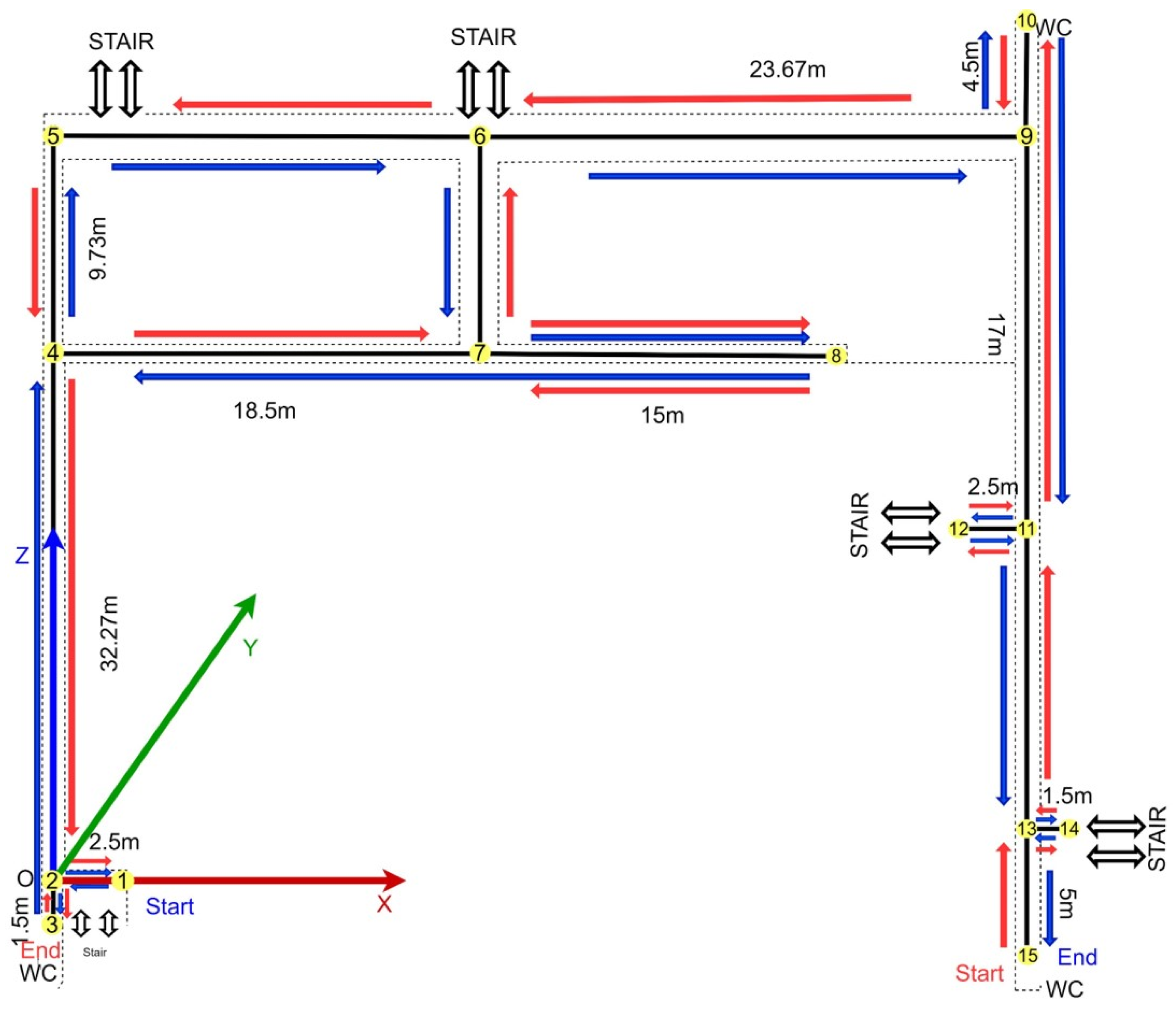
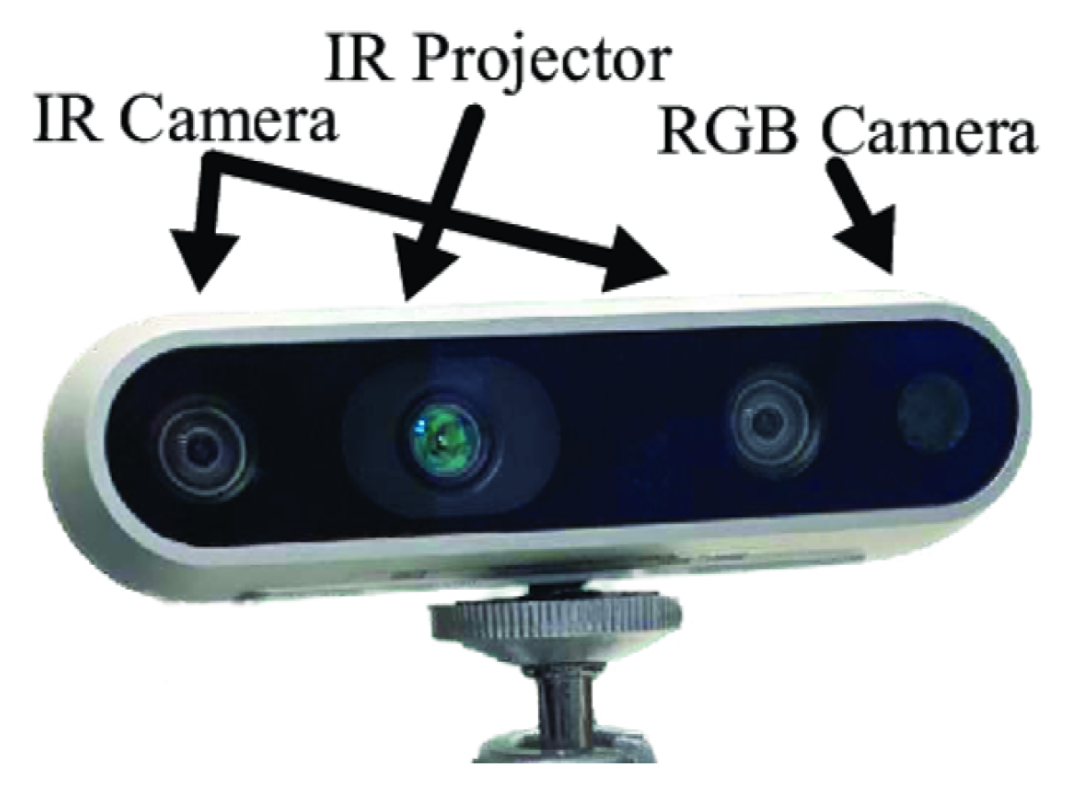
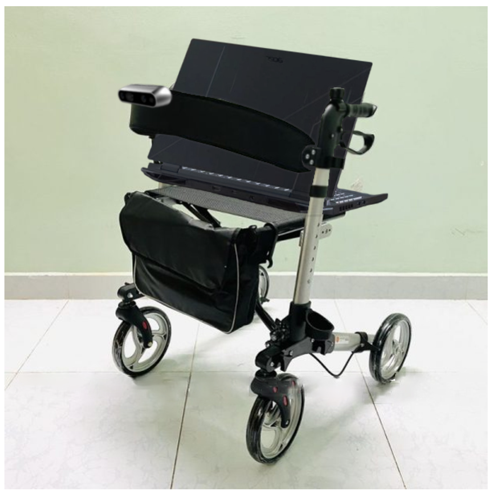
We set up the experiment in second-floor hallways of Building A, Building B, and Building C of Tan Trao University (TQU) in Vietnam, as illustrated in Figure 3. We called the “TQU-SLAM benchmark dataset”. Classrooms open onto these hallways. The data were collected from the environment using a Intel RealSense D435 camera (https://www.intelrealsense.com/depth-camera-d435/, accessed on 6 May 2024), illustrated in Figure 4. The camera was mounted on a vehicle, shown in Figure 5. The angle between the camera’s view and the ground was 45 degrees. For the total distance traveled by the vehicle at one time, the FO-D was 230.63 m and the OP-D was 228.13 m; the width was 2 m, and for every 0.5 m, we assigned a numbered marker with dimensions of 10 × 10 cm on each marked corner. The total number of markers we used was 332.
The moving speed to collect data was 0.2 m/s. The data we collected were color images and depth images with a resolution of 640 × 480 pixels. We always drove the car in the middle of the hallway. The data acquisition speed was 15 fps. We performed data collection four times in two days, each one hour apart. The first day, we collected data twice (1st, 2nd), and the second day, we collected the remaining two times (3rd, 4th). We collected data in the afternoon from 2:00 p.m. to 3:00 p.m. Each time, the direction of movement according to the blue arrow was in the forward direction (FO-D), and the direction of movement according to the red arrow was in the opposite direction (OP-D). All data of the TQU-SLAM benchmark dataset are shown in link (https://drive.google.com/drive/folders/16Dx_nORUvUHFg2BU9mm8aBYMvtAzE9m7, accessed on 6 May 2024). The data we collected are shown in Table 1.

3.2. Preparing Ground-Truth Trajectory for VO

To prepare the ground-truth data for evaluating the results of VO estimation, we built the ground-truth data of the motion trajectory as follows. We predefined a coordinate system in a real-world space as shown in Figure 3, where the X axis is red, the Y axis is green, and the Z axis is blue.
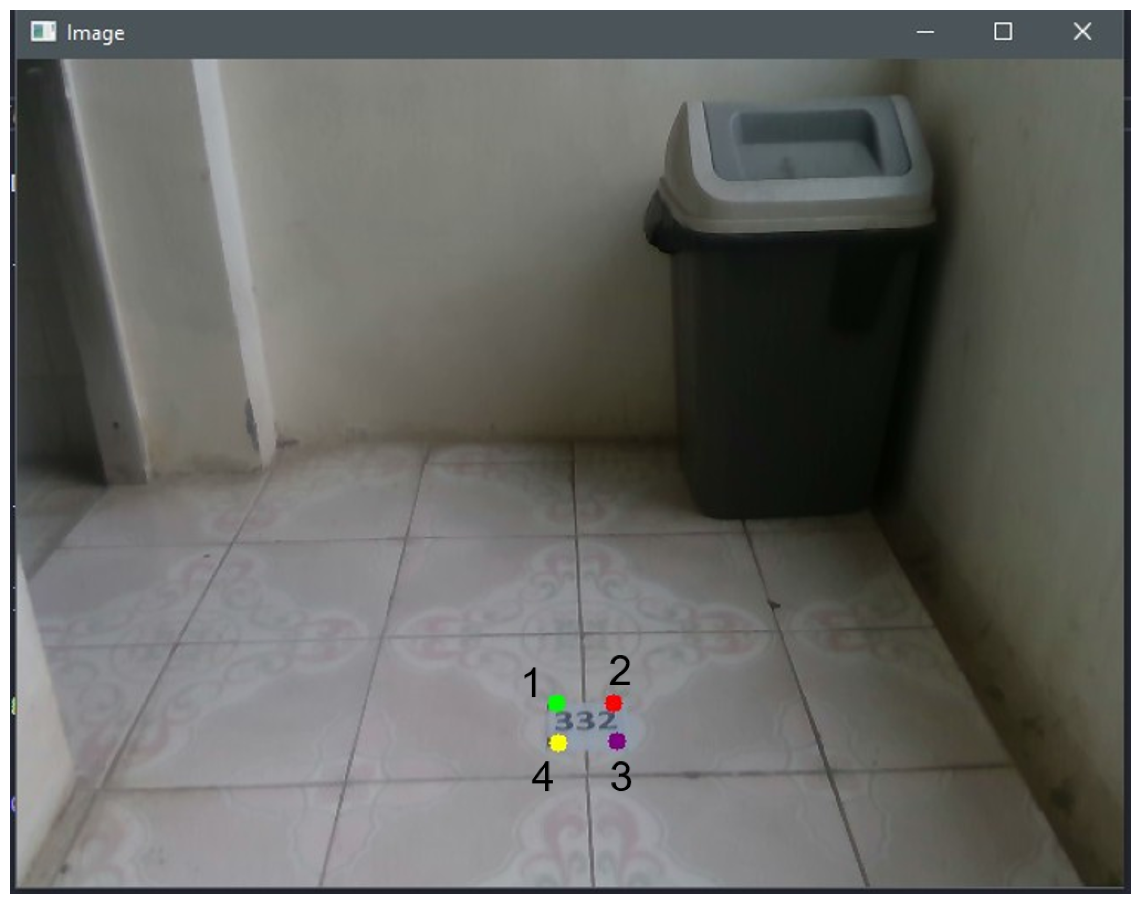
We used a self-developed tool in the Python programming language to mark four points on the color image, as shown in Figure 6. Then we took the corresponding four marker points on the depth image, because each frame was obtained as a pair of RGB images and depth images.
To convert the four marked points of the marker on the RGB image and the four corresponding points on the depth image to 3D point cloud data, we used the camera’s intrinsic parameters, shown in Equation (1):
f x 0 c x 0 f y c y 0 0 1 = 525.0 0 319.5 0 525.0 239.5 0 0 1
where f x , f y , c x , and c y are the intrinsic parameters of the camera. For each marker point with coordinates ( x d , y d ) and depth value d a on the depth image, the result is converted to point M with coordinates ( x m , y m , z m ) using Equation (2):
x m = ( x d c x ) × d a f x y m = ( y d c y ) × d a f y z m = d a
As shown in Figure 6, the four points of the marker point cloud data are according to the camera coordinate system, with the original coordinate system being the center of the camera. Therefore, to find these four points in the real-world coordinate system, it is necessary to find the rotation and translation matrix (transformation matrix) to transform four points from the camera coordinate system to the real-world coordinate system.
For a point with coordinates M ( x , y , z ) in the camera coordinate system, M ( x , y , z ) are the coordinates of point M in the real-world coordinate system, which we find after performing a transformation from the camera coordinate system to the real-world coordinate system using Equation (3):
x y z 1 = R o 11 R o 12 R o 13 T r 1 R o 21 R o 22 R o 23 T r 2 R o 31 R o 32 R o 33 T r 3 0 0 0 1 x y z 1
where R o 11 , R o 12 , R o 13 , R o 21 , R o 22 , R o 23 , R o 31 , R o 32 , R o 33 are the components of the rotation matrix from the camera coordinate system to the real-world coordinate system. T r 1 , T r 2 , and T r 3 are the components of the translation matrix from the camera coordinate system to the real-world coordinate system. The transformation result of point M is shown in Equation (4):
x = R o 11 x + R o 12 y + R o 13 z + T r 1 y = R o 21 x + R o 22 y + R o 23 z + T r 2 z = R o 31 x + R o 32 y + R o 33 z + T r 3
From the coordinates of the four points of point cloud data in the camera’s coordinate system, we define their coordinates in the matrix as Equation (5):
1 z 1 y 1 x 1 1 z 2 y 2 x 2 1 z 3 y 3 x 3 1 z 4 y 4 x 4
The transformation matrix according to the x , y , z axes is presented by θ 1 , θ 2 , θ 3 in Equation (6):
θ 1 = T r 1 R o 13 R o 12 R o 11 θ 2 = T r 2 R o 23 R o 22 R o 21 θ 3 = T r 3 R o 33 R o 32 R o 31
The results of the transformation are shown in the vector X , Y , Z in Equation (7):
X = x 1 x 2 x 3 x 4 Y = y 1 y 2 y 3 y 4 Z = z 1 z 2 z 3 z 4
where ( x 1 , y 1 , z 1 ) , ( x 2 , y 2 , z 2 ) , ( x 3 , y 3 , z 3 ) , ( x 4 , y 4 , z 4 ) are the coordinates of four points of point cloud data in the real-world coordinate system. From this, we have a linear equation, presented as Equation (8).
X = A × θ 1 Y = A × θ 2 Z = A × θ 3
To estimate θ 1 , θ 2 , θ 3 , we use the least squares method [46], as in Equation (9):
θ 1 = ( A T A ) 1 A T X θ 2 = ( A T A ) 1 A T Y θ 3 = ( A T A ) 1 A T Z
Finally, the conversion matrix between the camera coordinate system and the real-world coordinate system is of the form ( θ 1 ; θ 2 ; θ 3 ) . The coordinates of the center of the marker ( x c , y c , z c ) in the real-world coordinate system are calculated as Equation (10):
x c = x 1 + x 2 + x 3 + x 4 4 y c = y 1 + y 2 + y 3 + y 4 4 z c = z 1 + z 2 + z 3 + z 4 4
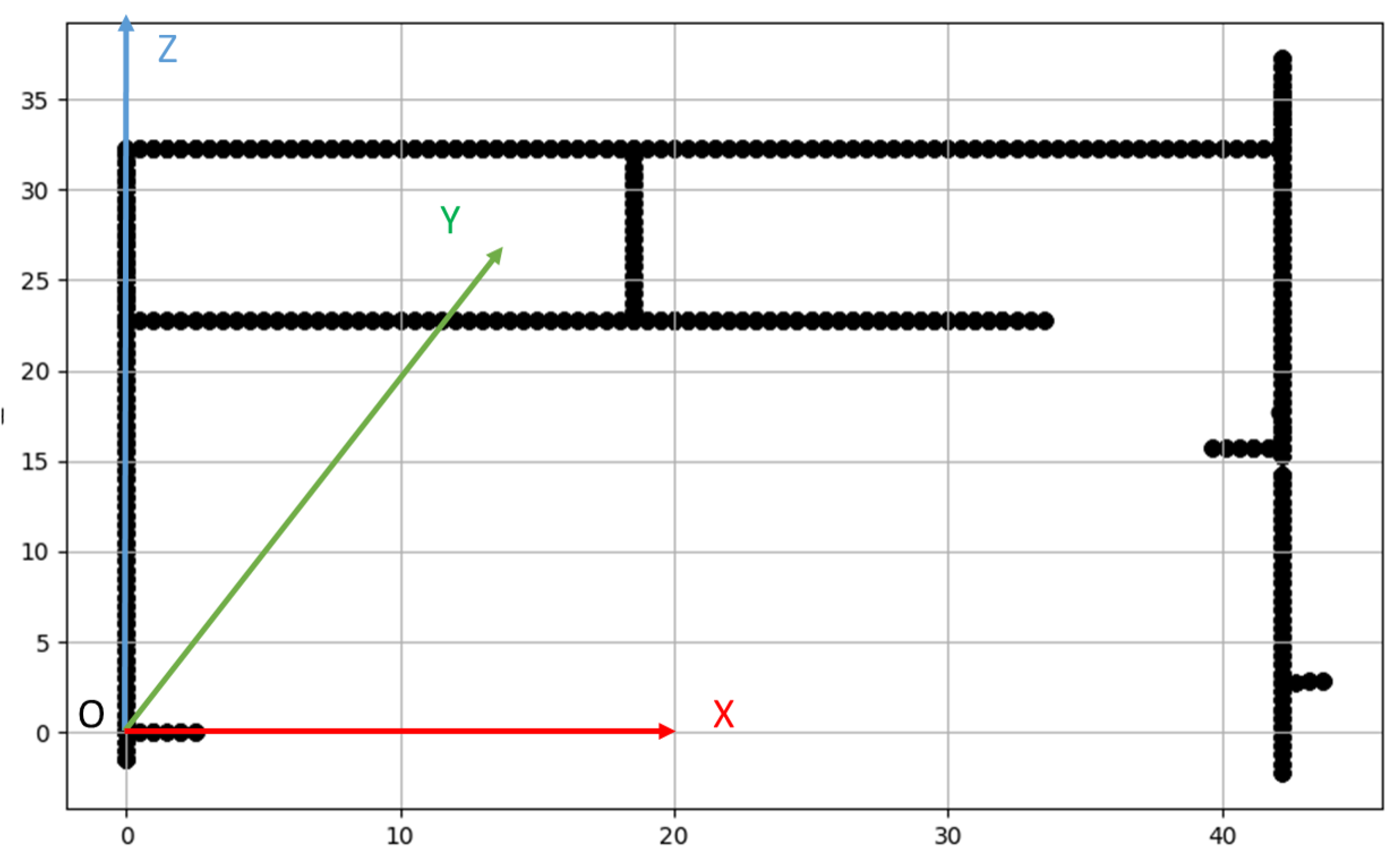
The ground-truth data results of the motion trajectory in the real-world coordinate system are shown in Figure 7.

4. Comparative Study of Building VO Based on Feature-Based Methods

As shown in Figure 1, the framework for constructing VO based on knowledge-based methods from the collected images of a monocular camera includes five steps. We present some recently published VO estimation techniques.

4.1. PySLAM

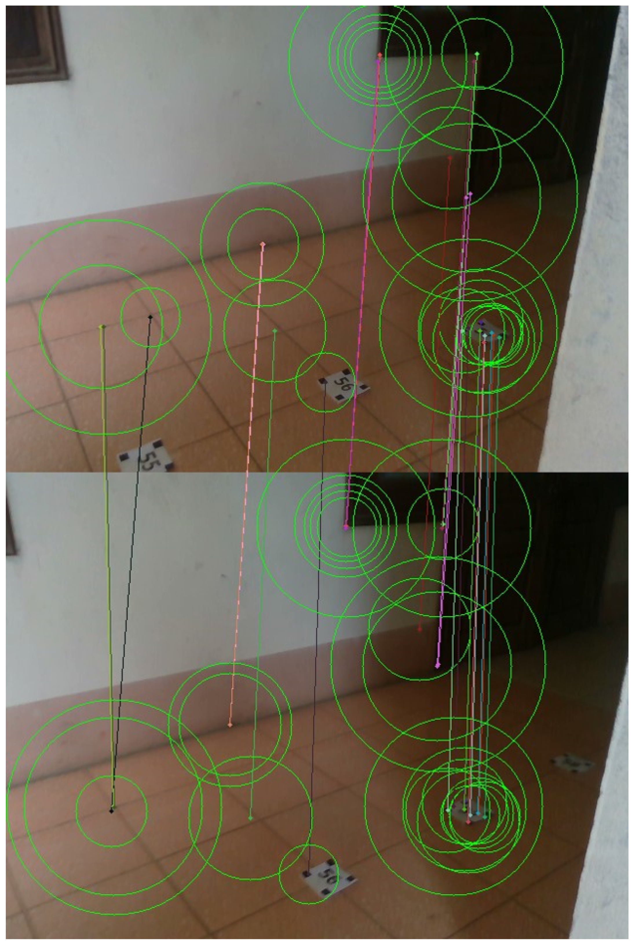
The PySLAM framework was proposed by Luigi [15,22]. It includes an open-source library developed for the PySLAM framework. The PySLAM framework allows the embedding of many types of features, including both traditional features automatically extracted from feature descriptors and DL features extracted from DL models. The source code of the PySLAM framework we used is shown in the link (https://github.com/luigifreda/pyslam, accessed on 6 May 2024). From there, it is possible to check and select good features for the process of building models to estimate a camera’s motion trajectory, helping to build pathfinding systems for robots and blind people. At the same time, PySLAM framework was developed in the C++ and Python programming languages. Just like the knowledge-based methods presented in Figure 1, the PySLAM framework also performs 6-DOF VO estimation with several steps. The feature-extraction step, or keypoint detection, comprises the process of detecting features/keypoints between two consecutive frames. The features can be edges, corners, or blobs. Typically, the features are detected and extracted according to a feature descriptor such as SHI_TOMASI, SIFT, SURF, ORB, ORB2, AKAZE, KAZE [18], or BRISK. At the same time, feature extraction through DL networks is also performed, for features such as VGG [19] and D2-Net [47]. Figure 8 shows the match between the corresponding ORB features in two consecutive frames of the TQU-SLAM benchmark dataset. The set of ORB features in two consecutive frames is small; the features can only be detected from the image area of the marker and railing in the moving journey. This also shows that the TQU-SLAM benchmark dataset contains many challenges for feature descriptors.
In the motion-estimation step, features are extracted from the monitored frame sequence, from which the camera motion is estimated through the transformation matrix in Equation (11):
T i , i 1 R o i , i 1 t i , i 1 0 1
where R o i , i 1 is the rotation matrix between two consecutive frames i and i 1 , and t i , i 1 is the translation vector between two consecutive frames i and i 1 .
The spatial correlation matrix between frames i and i 1 is calculated based on Equation (12):
E = α 0 t z t y t z 0 t x t y t x 0 R o
where t is a translation matrix in the x , y , z direction. The motion trajectory in 3D space is also calculated. A scale factor α is the shift factor between two consecutive frames.
The calculation of the essential matrix is performed in the epipolar plane system using “epipolar constraints”. To solve this problem, one can use the five-point algorithm, or 5-point RANSAC [22,48]. The RANSAC algorithm used here is to estimate the correspondence between two sets of keypoints. The points converted from the input set within a certain limit are called inliers. The algorithm iterates about K times [49] and outputs the largest number of inliers. K is calculated according to Equation (13):
K = l o g ( 1 p ) l o g ( 1 w s )
where p is the probability of finding a descriptors keypoints, s = 2 is the minimum number of samples needed to estimate a line model, and w is the likelihood ratio of the points being inliers.
In the local-optimization step, camera pose estimation and motion trajectory errors are accumulated from camera pose estimation and transformation. Currently, there are two methods commonly applied to optimize a camera’s movement trajectory in an environment. In the first method, the entire motion trajectory and camera pose are rechecked to minimize errors. The second method is to use the Kalman algorithm or particle filter to calibrate the map during data collection and edit the estimated camera pose when detecting new keypoints.

4.2. DPVO (Deep Patch Visual Odometry)

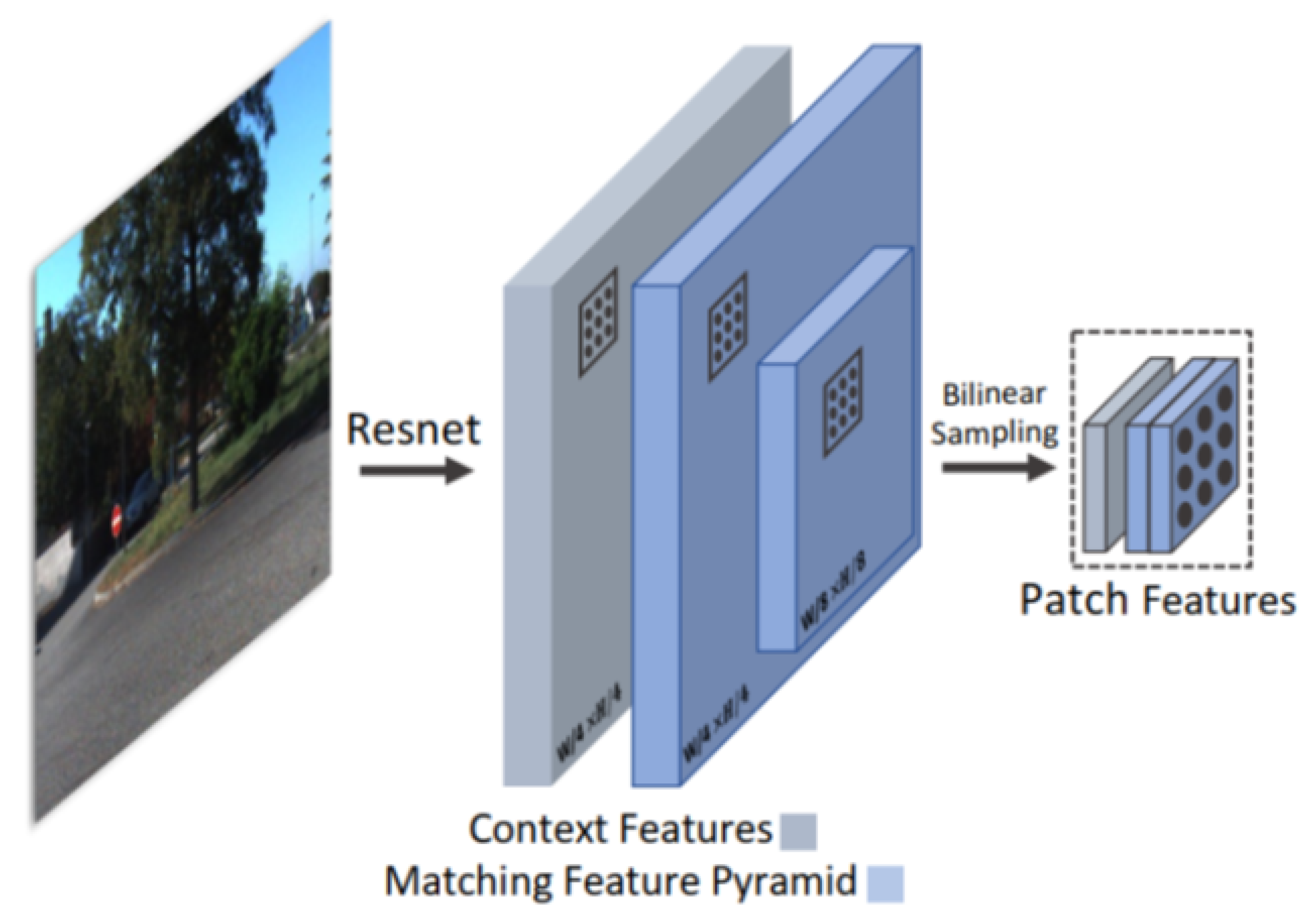
DPVO was proposed by Teed et al. [20]. DPVO is a deep learning framework that combines a CNN and a recurrent neural network (RNN). The architecture of DPVO is illustrated in Figure 9. With the input image data being an RGB image, DPVO performs per-pixel feature extraction using ResNet and uses it to calculate similarities between images in the frame sequence. Next, two residual networks are used: the first network is used to extract matching features, and the second network is used to extract contextual features. The first layer of each network performs convolution with a size of 7 × 7 , the next two residual blocks have a size of 32 × 32 , and the next two residual blocks have a size of 64 × 64 . Finally, the output of the feature vector is 1/4 the size of the input image. Next, a two-level feature pyramid is constructed with sizes 1/4 and 1/8, respectively, with the resolution of the input image based on a 4 × 4 filter with average pooling to the matching features to estimate the amount of optical flow.
Then, p × p patches are obtained from the feature map with random positions in the image space (pixel space) using the bilinear sampling technique. The patches map is created by linking patches, and it has the same size as the feature map with regard to pixels. Furthermore, DPVO uses a patch graph to represent the relationship between patches and video frames. The projections of patches on the frames are the patches’ movement trajectories. At the same time, DPVO also proposes an update operator that is a recurrent network that iteratively fine-tunes the depth of each patch and the camera pose of each frame in the video. DPVO is rated to be 3x faster than DROID-SLAM [50]. In DPVO, the model is trained from several datasets such as the TartanAir [51], TUM RGB-D SLAM [12], EuRoC [52], and ICL-NUIM [14] datasets.

4.3. TartanVO

TartanVO was proposed by Wang et al. [21]. This network has an architecture consisting of two stages: the first is a matching network to match the features between two consecutive frames ( i 1 , i ) , thereby estimating the optical flow. Second, the pose network is used to predict the camera pose based on the estimated optical flow. The architecture of TartanVO is shown in Figure 10.
In the TartanVO model, the authors built a pretrained model trained on large datasets: the EuRoC [52], KITTI [9,10,11], Cityscapes [45], and TartanAir [51] datasets. From these, they enriched the contexts and environmental conditions in which the model was trained. To increase the model’s generalization ability, TartanVO proposes two up-to-scale loss functions. The first is the cosine similarity loss to calculate the cosine angle between the estimated translation and the displacement label. The second is the normalized distance loss to calculate the distance between the estimated translation vector and translation label.

5. Experimental Results

5.1. Evaluation Measures

To evaluate the results of the VO algorithm based on feature-based methods, we use several evaluation metrics as follows:
  • The absolute trajectory error ( A T E ) [12] is the distance error between the ground-truth A T ^ i and the estimated motion A T i trajectory, aligned with an optimal S E ( 3 ) pose T . A T E is calculated according to Equation (14):
    A T E = min T S E ( 3 ) 1 I g t | i I g t | | T A T i A T ^ i | | 2
    where t r e l is the average translations R M S E drift (%) on a length of 100–800 m. r r e l is the average rotational RMSE drift (°/100 m) on a length of 100–800 m.
  • We calculate trajectory error ( E r r d ), being the distance error between the ground-truth A T ^ i and the estimated motion A T i trajectory. E r r d is calculated according to Equation (15):
    E r r d = 1 N | | A T i A T ^ i | | 2
    where N is the frame number of the frame sequence used to estimate the camera’s motion trajectory.
  • In addition, we also calculate the ratio of the number of frames with detected keypoints ( r d (%)).

5.2. Evaluation Parameters

In this paper, we use the PySLAM framework [22], with all the features integrated into this framework. PySLAM’s development source code is in Python v3.9 language and programmed on Ubuntu 20.04. For the DPVO build source code, we used the code at the link (https://github.com/princeton-vl/DPVO, accessed on 6 May 2024). For the TartanVO build source code, we used the code at the link (https://github.com/castacks/tartanvo, accessed on 6 May 2024). At the same time, there is support from several open-source libraries such as Numpy (1.18.2), OpenCV (4.5.1), PyTorch (≥1.4.0), and Tensorflow-gpu (1.14.0). The PySLAM framework was implemented on computers with the following configuration: CPU i5 12,400 f, 16 G DDr4, GPU RTX 3060 12 GB. In this paper, with the DPVO and TartanVO networks, we performed three experiments ( L 1 , L 2 , L 3 ) with each subset of the TQU-SLAM benchmark dataset for estimating the camera motion trajectory. The results are shown in the next section.

5.3. Results and Discussions

The results of estimating VO/camera pose/camera trajectory using the TQU-SLAM benchmark dataset when using SHI_TOMASI, SIFT, SURF, ORB, ORB2, AKAZE, KAZE [18], BRISK, and VGG to extract features are shown in Table 2. The average distance error of the ORB2 feature is the lowest ( E r r d = 5.74 mm).
The ratio of detected and extracted frames characterized for 6-DOF camera pose estimation is shown in Table 3. The average ratio of detected frames with the SHI_TOMASI feature is the highest ( r d = 98.97 % ).
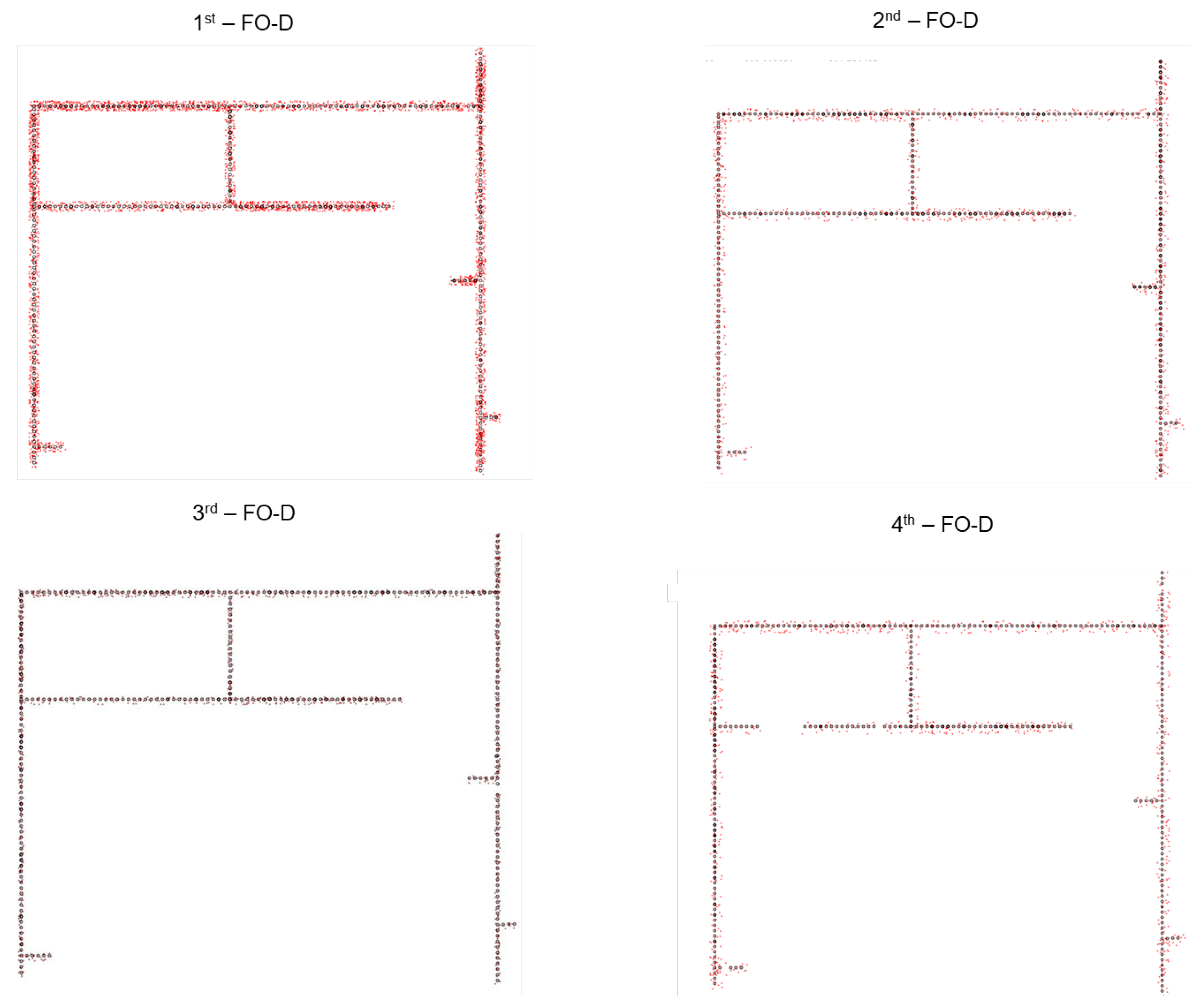
Figure 11 shows the results of estimating the VO of FO-D of the TQU-SLAM benchmark dataset when using the SHI_TOMASI features extracted from RGB images. Figure 11 also shows that SHI_TOMASI features are extracted better and more in the first FO-D compared to data at other times.
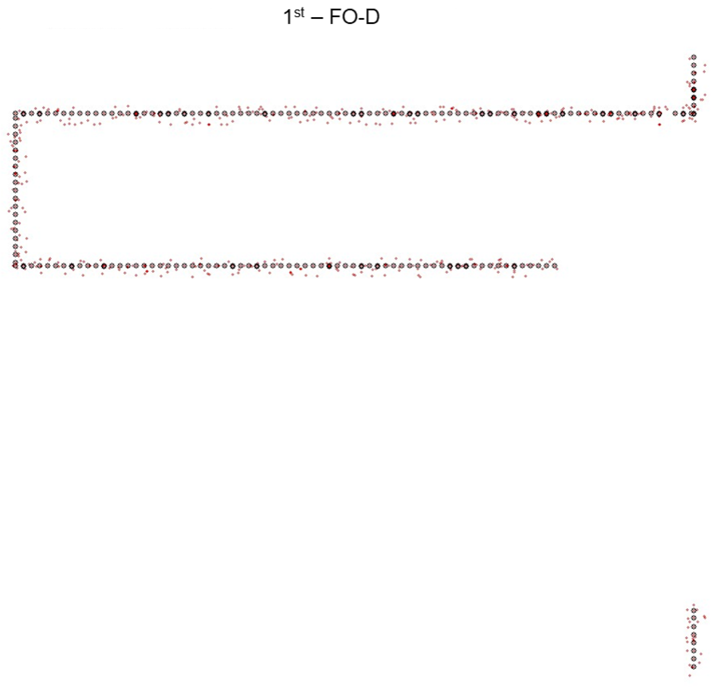
Figure 12 shows the results of estimating points on the moving trajectory on the 1st-FO-D of the TQU-SLAM benchmark dataset when using the features extracted from VGG.
The results in Figure 12 also show that the features extracted are limited when using VGG; there are many frames whose features cannot be extracted. Therefore, the camera’s position cannot be estimated. Figure 13 shows the difficult feature extraction in frame pairs when using VGG for feature extraction.
The results of the camera motion trajectory estimation error ( E r r d ) based on the DPVO and TartanVO networks on the TQU-SLAM benchmark dataset are shown in Table 4.
The results of the camera motion trajectory estimation error ( A T E ) based on the DPVO and TartanVO networks on the TQU-SLAM benchmark dataset are shown in Table 5.
The ratio of the number of detected and extracted frames characterized to estimate the VO of the DPVO is shown in Table 6. This rate is low, only 49.68%, while the characteristic extraction rate of the TartanVO is 100%.
As shown in Table 4, the average estimation error ( E r r d ) of DPVO is 13.7 m, and the ( E r r d ) of TartanVO is 14.96 m. Table 5 also shows that the average estimation error ( A T E ) of DPVO is 15.96 m, and the ( A T E ) of TartanVO is 17.46 m. These results show that DPVO is better than TartanVO in the estimation error, but the estimated realized frame rate of DPVO is only 49.68%.
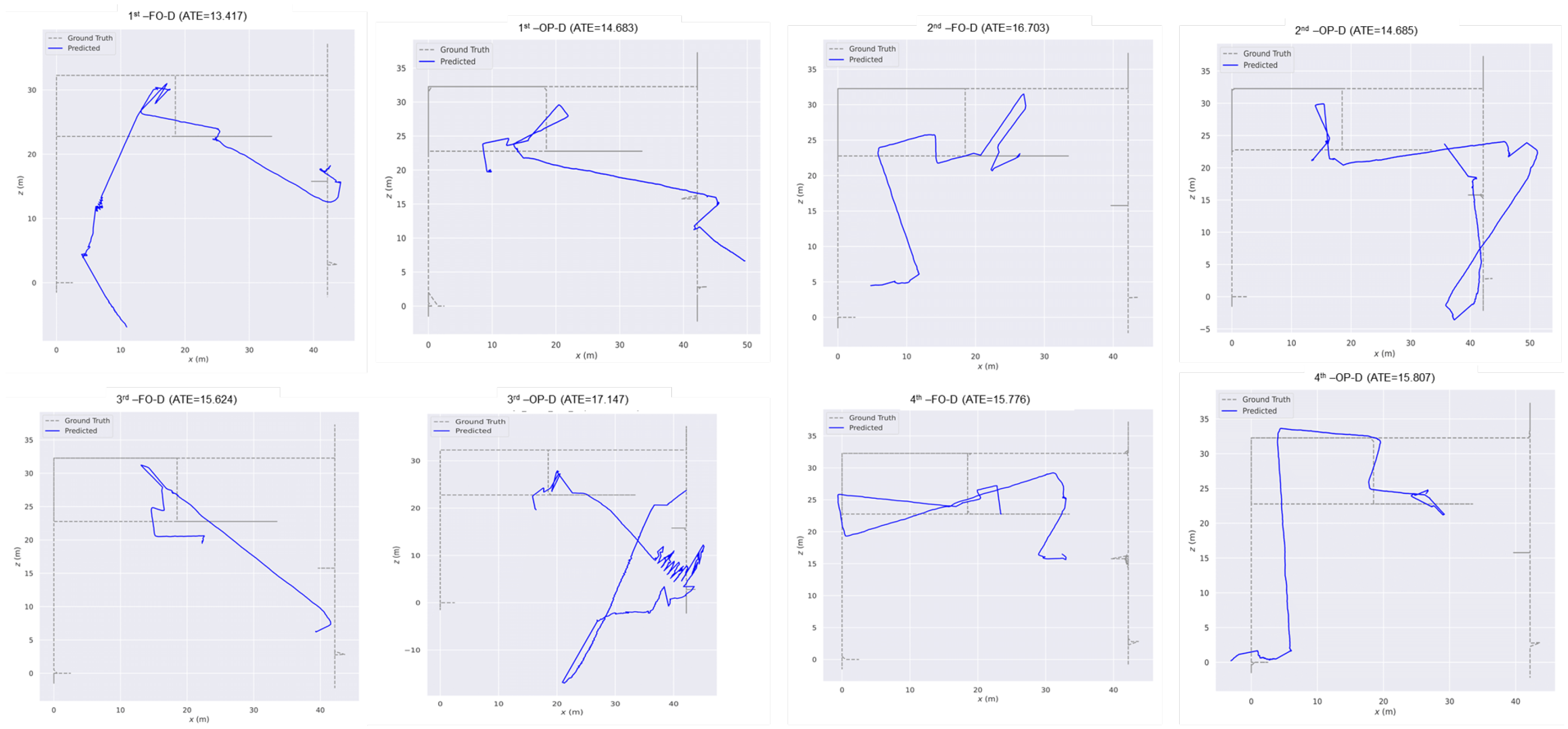
Figure 14 shows the results of estimating the camera’s motion trajectory based on the DPVO model when experimenting with L 1 of the TQU-SLAM benchmark dataset.
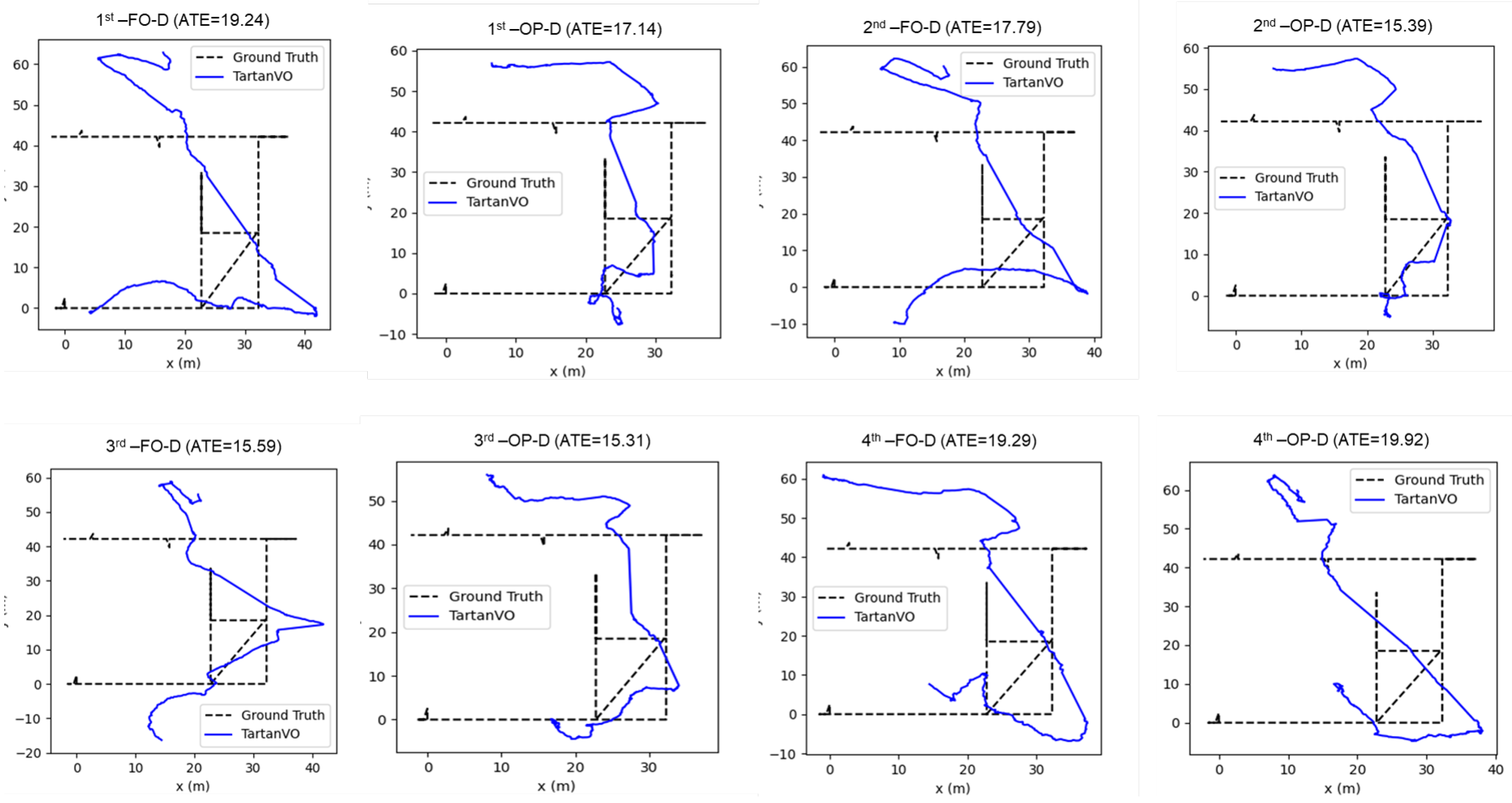
Figure 15 shows the results of estimating the camera’s motion trajectory based on the TartanVO model when experimenting with L 1 of the TQU-SLAM benchmark dataset.

5.4. Challenges

As shown in Figure 11, Figure 12, Figure 13 and Table 3, the TQU-SLAM benchmark dataset contains some challenges for VO construction as follows. Firstly, regarding lighting conditions, the obtained RGB images have very weak lighting conditions, and the light intensity is uneven. There are road sections with adequate lighting, but there are road sections where we had to use additional light from mobile phone lights to assist, as shown in Figure 13. Therefore, the keypoints between two consecutive frames are not detected. Second, the collected environment is highly homogeneous. The image data obtained by the Intel RealSense D435 are mainly floor data and a small part are wall and railing data. Therefore, the data do not have great discrimination between frames; in the scene, there are few objects in the environment. Although we posted markers on the floor, the number of keypoints detected in the two frames is not high. This leads to a failure to estimate the 6-DOF camera poses across multiple frames. Although, the DPVO and TartanVO networks were pretrained on many large datasets such as the EuRoC [52], KITTI [9,10,11], Cityscapes [45], and TartanAir [51] datasets, when performing feature extraction on the TQU-SLAM benchmark dataset, there is a large number of frames that cannot be detected and whose features cannot be extracted (more than 50% of DPVO). The results are shown in Table 4, Table 5 and Table 6. Figure 14 and Figure 15 illustrate that the misestimation results of DPVO and TartanVO are very large. This proves that the problem of data enrichment to train the VO estimation model still contains many challenges that need to be implemented.

6. Conclusions and Future Works

VO systems are widely applied in pathfinding robots, autonomous vehicles operating in industry, etc. DL has had impressive results in building visual SLAM and VO systems. However, DL requires a large amount of data to train the model. In this paper, we introduced the TQU-SLAM benchmark dataset, collected from an RGB-D image sensor (Intel RealSense D435) moving in the corridors of three buildings of a particular length (FO-D is 230.63 m, OP-D is 228.13 m). The ground-truth data of the TQU-SLAM benchmark dataset include 6-DOF camera poses/camera trajectory and a 3D point cloud. It was also tested to estimate VO using some traditional features and features extracted from DL, such as VGG based on the PySLAM framework. Among them, the ORB2 features have the best results ( E r r d = 5.74 mm), and the ratio of the number of frames with detected keypoints of the SHI_TOMASI feature is the best ( r d = 98.97 % ). Shortly, we will renormalize the TQU-SLAM benchmark dataset and prepare many types of ground-truth data for evaluating visual SLAM and VO models. We will build a pretrained model on the TQU-SLAM benchmark dataset and perform comparative research on DL models for visual SLAM and VO systems.

Author Contributions

Methodology, T.-H.N. and V.-H.L.; Writing—original draft, T.-H.N., V.-H.L., H.-S.D., T.-H.T. and V.-N.P.; Writing—review & editing, V.-H.L. and H.-S.D.; Visualization, H.-S.D., T.-H.T. and V.-N.P.; Supervision, V.-H.L. All authors have read and agreed to the published version of the manuscript.

Funding

This research is supported by Hung Vuong University under grant number HV23.2023.

Data Availability Statement

The data presented in this study are available in this paper.

Conflicts of Interest

The paper is our research, not related to any organization or individual. It is part of a series of studies on visual SLAM and VO systems.

References

  1. Wang, K.; Ma, S.; Chen, J.; Ren, F.; Lu, J. Approaches, Challenges, and Applications for Deep Visual Odometry: Toward Complicated and Emerging Areas. IEEE Trans. Cogn. Dev. Syst. 2022, 14, 35–49. [Google Scholar] [CrossRef]
  2. Neyestani, A.; Picariello, F.; Basiri, A.; Daponte, P.; Vito, L.D. Survey and research challenges in monocular visual odometry. In Proceedings of the 2023 IEEE International Workshop on Metrology for Living Environment, MetroLivEnv 2023, Milano, Italy, 29–31 May 2023; pp. 107–112. [Google Scholar] [CrossRef]
  3. Agostinho, L.R.; Ricardo, N.M.; Pereira, M.I.; Hiolle, A.; Pinto, A.M. A Practical Survey on Visual Odometry for Autonomous Driving in Challenging Scenarios and Conditions. IEEE Access 2022, 10, 72182–72205. [Google Scholar] [CrossRef]
  4. Low, D.G. Distinctive image features from scale-invariant keypoints. Int. J. Comput. Vis. 2004, 60, 91–110. [Google Scholar] [CrossRef]
  5. Bay, H.; Tuytelaars, T.; Van Gool, L. SURF: Speeded up robust features. In Proceedings of the Lecture Notes in Computer Science (Including Subseries Lecture Notes in Artificial Intelligence and Lecture Notes in Bioinformatics), Redondo Beach, CA, USA, 8–11 July 2006; Volume 3951 LNCS, pp. 404–417. [Google Scholar] [CrossRef]
  6. Rublee, E.; Rabaud, V.; Konolige, K.; Bradski, G. ORB: An efficient alternative to SIFT or SURF. In Proceedings of the IEEE International Conference on Computer Vision, Colorado Springs, CO, USA, 20–25 June 2011; pp. 2564–2571. [Google Scholar] [CrossRef]
  7. Leutenegger, S.; Chli, M.; Siegwart, R.Y. BRISK: Binary robust invariant scalable keypoints. In Proceedings of the IEEE International Conference on Computer Vision, Venice, Italy, 22–29 October 2011; pp. 2548–2555. [Google Scholar] [CrossRef]
  8. Lucas, B.D.; Kanade, T. An iterative image registration technique with an application to stereo vision. In Proceedings of the IJCAI’81: Proceedings of the 7th International Joint Conference on Artificial Intelligence, Vancouver, BC, Canada, 24–28 August 1981; pp. 674–679. [Google Scholar]
  9. Geiger, A.; Lenz, P.; Urtasun, R. Are we ready for autonomous driving? The KITTI vision benchmark suite. In Proceedings of the Conference on Computer Vision and Pattern Recognition (CVPR), Seattle, WA, USA, 14–19 June 2012. [Google Scholar]
  10. Geiger, A.; Lenz, P.; Stiller, C.; Urtasun, R. Vision meets robotics: The KITTI dataset. Int. J. Robot. Res. 2013, 32, 1231–1237. [Google Scholar] [CrossRef]
  11. Menze, M.; Geiger, A. Object scene flow for autonomous vehicles. In Proceedings of the Conference on Computer Vision and Pattern Recognition (CVPR), Boston, MA, USA, 7–12 June 2015. [Google Scholar]
  12. Sturm, J.; Engelhard, N.; Endres, F.; Burgard, W.; Cremers, D. A benchmark for the evaluation of RGB-D SLAM systems. In Proceedings of the 2012 IEEE/RSJ International Conference on Intelligent Robots and Systems, Vilamoura-Algarve, Portugal, 7–12 October 2012; Volume 32, pp. 315–326. [Google Scholar] [CrossRef]
  13. Silberman, N.; Hoiem, D.; Kohli, P.; Fergus, R. Indoor Segmentation and Support Inference from RGBD Images. Comput. Vis. ECCV2012 2012, 7578, 1–14. [Google Scholar]
  14. Handa, A.; Whelan, T.; McDonald, J.; Davison, A.J. A benchmark for RGB-D visual odometry, 3D reconstruction and SLAM. In Proceedings of the IEEE International Conference on Robotics and Automation, Hong Kong, China, 31 May–7 June 2014; pp. 1524–1531. [Google Scholar] [CrossRef]
  15. Hodne, L.M.; Leikvoll, E.; Yip, M.; Teigen, A.L.; Stahl, A.; Mester, R. Detecting and Suppressing Marine Snow for Underwater Visual SLAM. IEEE Comput. Soc. Conf. Comput. Vis. Pattern Recognit. Work. 2022, 2022, 5097–5105. [Google Scholar] [CrossRef]
  16. Mur-Artal, R.; Montiel, J.M.; Tardos, J.D. ORB-SLAM: A Versatile and Accurate Monocular SLAM System. IEEE Trans. Robot. 2015, 31, 1147–1163. [Google Scholar] [CrossRef]
  17. Mur-Artal, R.; Tardos, J.D. ORB-SLAM2: An Open-Source SLAM System for Monocular, Stereo and RGB-D Cameras. IEEE Trans. Robot. 2017, 33, 1255–1262. [Google Scholar] [CrossRef]
  18. Alcantarilla, P.F.; Bartoli, A.; Davison, A.J. KAZE features. Lect. Notes Comput. Sci. Including Subser. Lect. Notes Artif. Intell. Lect. Notes Bioinformatics 2012, 7577, 214–227. [Google Scholar] [CrossRef]
  19. Simonyan, K.; Zisserman, A. Very deep convolutional networks for large-scale image recognition. In Proceedings of the 3rd International Conference on Learning Representations, ICLR 2015—Conference Track Proceedings, San Diego, CA, USA, 7–9 May 2015; pp. 1–14. [Google Scholar]
  20. Teed, Z.; Lipson, L.; Deng, J. Deep Patch Visual Odometry. Available online: https://proceedings.neurips.cc/paper_files/paper/2023/hash/7ac484b0f1a1719ad5be9aa8c8455fbb-Abstract-Conference.html (accessed on 6 May 2024).
  21. Wang, W.; Hu, Y.; Scherer, S. TartanVO: A generalizable learning-based VO. In Proceedings of the Conference on Robot Learning, Online, 16–18 November 2020. [Google Scholar]
  22. Freda, L. pySLAM Contains a Monocular Visual Odometry (VO) Pipeline in Python. 2024. Available online: https://github.com/luigifreda/pyslam (accessed on 5 April 2024).
  23. He, M.; Zhu, C.; Huang, Q.; Ren, B.; Liu, J. A review of monocular visual odometry. Vis. Comput. 2020, 36, 1053–1065. [Google Scholar] [CrossRef]
  24. Davison, A.J.; Reid, I.D.; Molton, N.D.; Stasse, O. MonoSLAM: Real-Time Single Camera SLAM. IEEE Trans. Pattern Anal. Mach. Intell. 2007, 104, 1292–1296. [Google Scholar] [CrossRef]
  25. Klein, G.; Murray, D. Parallel tracking and mapping for small AR workspaces. In Proceedings of the 2007 6th IEEE and ACM International Symposium on Mixed and Augmented Reality, ISMAR, Nara, Japan, 13–16 November 2007; pp. 225–234. [Google Scholar] [CrossRef]
  26. Ganai, M.; Lee, D.; Gupta, A. DTAM: Dense tracking and mapping in real-time. In Proceedings of the The International Conference on Computer Vision (ICCV), Online, 6–13 November 2012; pp. 1–11. [Google Scholar] [CrossRef]
  27. Izadi, S.; Kim, D.; Hilliges, O.; Molyneaux, D.; Newcombe, R.; Kohli, P.; Shotton, J.; Hodges, S.; Freeman, D.; Davison, A.; et al. KinectFusion: Real-time 3D reconstruction and interaction using a moving depth camera. In Proceedings of the 24th Annual ACM Symposium on User Interface Software and Technology, Santa Barbara, CA, USA, 16–19 October 2011; Volume 11. [Google Scholar]
  28. Kerl, C.; Sturm, J.; Cremers, D. Dense visual SLAM for RGB-D cameras. In Proceedings of the 2013 IEEE/RSJ International Conference on Intelligent Robots and Systems, Tokyo, Japan, 3–7 November 2013; Volume 41, pp. 306–308. [Google Scholar] [CrossRef]
  29. Forster, C.; Pizzoli, M.; Scaramuzza, D. SVO: Fast semi-direct monocular visual odometry. In Proceedings of the IEEE International Conference on Robotics and Automation, Hong Kong, China, 31 May–7 June 2014. [Google Scholar]
  30. Bloesch, M.; Omari, S.; Hutter, M.; Siegwart, R. Robust visual inertial odometry using a direct EKF-based approach. In Proceedings of the 2015 IEEE/RSJ International Conference on Intelligent Robots and Systems (IROS), Hamburg, Germany, 28 September–2 October 2015. [Google Scholar]
  31. Bloesch, M.; Burri, M.; Omari, S.; Hutter, M.; Siegwart, R. IEKF-based Visual-Inertial Odometry using Direct Photometric Feedback. Int. J. Robot. Res. 2017, 36, 106705. [Google Scholar] [CrossRef]
  32. Whelan, T.; Leutenegger, S.; Salas-Moreno, R.F.; Glocker, B.; Davison, A.J. ElasticFusion: Dense SLAM without a pose graph. Robot. Sci. Syst. 2015, 11, 3. [Google Scholar] [CrossRef]
  33. Whelan, T.; Salas-Moreno, R.F.; Glocker, B.; Davison, A.J.; Leutenegger, S. ElasticFusion: Real-time dense SLAM and light source estimation. Int. J. Robot. Res. 2016, 35, 1697–1716. [Google Scholar] [CrossRef]
  34. Engel, J.; Koltun, V.; Cremers, D. Direct Sparse Odometry. IEEE Trans. Pattern Anal. Mach. Intell. 2018, 40, 611–625. [Google Scholar] [CrossRef]
  35. Campos, C.; Elvira, R.; Rodríguez, J.J.G.; Montiel, J.M.; Tardós, J.D. ORB-SLAM3: An Accurate Open-Source Library for Visual, Visual. IEEE Trans. Robot. 2021, 37, 1874–1890. [Google Scholar] [CrossRef]
  36. Schneider, T.; Dymczyk, M.; Fehr, M.; Egger, K.; Lynen, S.; Gilitschenski, I.; Siegwart, R. Maplab: An Open Framework for Research in Visual-Inertial Mapping and Localization. IEEE Robot. Autom. Lett. 2018, 3, 1418–1425. [Google Scholar] [CrossRef]
  37. Huang, W.; Wan, W.; Liu, H. Optimization-based online initialization and calibration of monocular visual-inertial odometry considering spatial-temporal constraints. Sensors 2021, 21, 2673. [Google Scholar] [CrossRef]
  38. Zhou, L.; Wang, S.; Kaess, M. DPLVO: Direct Point-Line Monocular Visual Odometry. IEEE Robot. Autom. Lett. 2021, 6, 1–8. [Google Scholar] [CrossRef]
  39. Ban, X.; Wang, H.; Chen, T.; Wang, Y.; Xiao, Y. Monocular Visual Odometry Based on Depth and Optical Flow Using Deep Learning. IEEE Trans. Instrum. Meas. 2021, 70, 1–19. [Google Scholar] [CrossRef]
  40. Lin, L.; Wang, W.; Luo, W.; Song, L.; Zhou, W. Unsupervised monocular visual odometry with decoupled camera pose estimation. Digit. Signal Process. Rev. J. 2021, 114, 103052. [Google Scholar] [CrossRef]
  41. Gadipudi, N.; Elamvazuthi, I.; Lu, C.K.; Paramasivam, S.; Su, S. WPO-net: Windowed pose optimization network for monocular visual odometry estimation. Sensors 2021, 21, 8155. [Google Scholar] [CrossRef] [PubMed]
  42. Kim, U.H.; Kim, S.H.; Kim, J.H. SimVODIS: Simultaneous Visual Odometry, Object Detection, and Instance Segmentation. IEEE Trans. Pattern Anal. Mach. Intell. 2022, 44, 428–441. [Google Scholar] [CrossRef] [PubMed]
  43. Turan, Y.A.M.; Sarı, A.E.; Saputra, M.R.U.; de Gusmo, P.P.B.; Markham, A.; Trigoni, N. SelfVIO: Self-Supervised Deep Monocular Visual-Inertial Odometry and Depth Estimation. Neurocomputing 2021, 421, 119–136. [Google Scholar]
  44. Saxena, A.; Sun, M.; Ng, A.Y. Make3D: Learning 3D scene structure from a single still image. IEEE Trans. Pattern Anal. Mach. Intell. 2009, 31, 824–840. [Google Scholar] [CrossRef] [PubMed]
  45. Ramos, S.; Rehfeld, T.; Enzweiler, M.; Benenson, R.; Roth, S. The cityscapes dataset for semantic urban scene understanding. In Proceedings of the CVPR, Las Vegas, NV, USA, 27–30 June 2016. [Google Scholar]
  46. Linear. Linear Regression. Available online: https://machinelearningcoban.com/2016/12/28/linearregression/ (accessed on 5 April 2024).
  47. Dusmanu, M.; Rocco, I.; Pajdla, T.; Pollefeys, M.; Sivic, J.; Torii, A.; Sattler, T. D2-Net: A trainable CNN for joint detection and description of local features. In Proceedings of the 2019 IEEE/CVF Conference on Computer Vision and Pattern Recognition, Long Beach, CA, USA, 15–20 June 2019. [Google Scholar]
  48. Fraundorfer, F.; Scaramuzza, D. Visual odometry: Part II: Matching, robustness, optimization, and applications. IEEE Robot. Autom. Mag. 2012, 19, 78–90. [Google Scholar] [CrossRef]
  49. Le, V.H.; Vu, H.; Nguyen, T.T.; Le, T.L.; Tran, T.H. Acquiring qualified samples for RANSAC using geometrical constraints. Pattern Recognit. Lett. 2018, 102, 58–66. [Google Scholar] [CrossRef]
  50. Teed, Z.; Deng, J. DROID-SLAM: Deep Visual SLAM for Monocular, Stereo, and RGB-D Cameras. Adv. Neural Inf. Process. Syst. 2021, 20, 16558–16569. [Google Scholar]
  51. Wang, W.; Zhu, D.; Wang, X.; Hu, Y.; Qiu, Y.; Wang, C.; Hu, Y.; Kapoor, A.; Scherer, S. TartanAir: A dataset to push the limits of visual SLAM. In Proceedings of the International Conference on Intelligent Robots and Systems (IROS), International Conference on Intelligent Robots and Systems (IROS), Las Vegas, NV, USA, 24 October 2020–24 January 2021. [Google Scholar]
  52. Burri, M.; Nikolic, J.; Gohl, P.; Schneider, T.; Rehder, J.; Omari, S.; Achtelik, M.W.; Siegwart, R. The EuRoC micro aerial vehicle datasets. Int. J. Robot. Res. 2016, 35, 1157–1163. Available online: http://ijr.sagepub.com/content/early/2016/01/21/0278364915620033.full.pdf+html (accessed on 6 May 2024). [CrossRef]
Figure 1. VO framework to build camera motion trajectory from image sequence.
Futureinternet 16 00174 g001
Figure 2. The tree of the methods to build VO from images obtained from a camera.
Futureinternet 16 00174 g002
Figure 3. Illustration of the hallway environment of Building A, Building B, and Building C of Tan Trao University in Vietnam for data collection. In the environment, we highlight 15 keypoints. The direction of movement according to the blue arrow is in the forward direction, and the direction of movement according to the red arrow is in the opposite direction.
Futureinternet 16 00174 g003
Figure 4. Illustration of an Intel RealSense D435 camera with an infrared projector, a color (RGB) camera, and two cameras to collect stereo depth (D) images.
Futureinternet 16 00174 g004
Figure 5. Illustration of a vehicle equipped with a camera and computer when collecting data.
Futureinternet 16 00174 g005
Figure 6. Illustration of marker application and the marker results collected on a color image.
Futureinternet 16 00174 g006
Figure 7. Illustration of the real-world coordinate system we defined and the camera’s motion trajectory. The ground truth of the camera’s motion trajectory is the black points.
Futureinternet 16 00174 g007
Figure 8. Illustration of ORB feature matching of two consecutive frames from the TQU-SLAM benchmark dataset.
Futureinternet 16 00174 g008
Figure 9. Illustration of DPVO architecture.
Futureinternet 16 00174 g009
Figure 10. Illustration of TartanVO architecture [21].
Futureinternet 16 00174 g010
Figure 11. Illustration of the results of estimating VO of TQU-SLAM benchmark dataset when using the SHI_TOMASI features. The results are presented on FO-D data. The black points belong to the ground-truth trajectory, and the red points are the estimated camera position.
Futureinternet 16 00174 g011
Figure 12. Illustration of the results of estimating VO of the first FO-D of the TQU-SLAM benchmark dataset when using the features extracted by VGG. The black points belong to the ground-truth trajectory, and the red points are the estimated camera position.
Futureinternet 16 00174 g012
Figure 13. Illustration of the feature matching extracted from the VGG of frame pair of 1st FO-D of the TQU-SLAM benchmark dataset. The lines connecting two features on two consecutive frames represent two corresponding locations on two consecutive frames detected by the feature descriptor.
Futureinternet 16 00174 g013
Figure 14. Illustration of the results of estimating the camera’s moving trajectory on the TQU-SLAM benchmark dataset when using the DPVO model. The ground-truth motion trajectory is the black line, and the estimated trajectory of the DPVO model is the blue line.
Futureinternet 16 00174 g014
Figure 15. Illustration of the results of estimating the camera’s moving trajectory on the TQU-SLAM benchmark dataset when using the TartanVO model. The ground-truth motion trajectory is the black line, and the estimated trajectory of the TartanVO model is the blue line.
Futureinternet 16 00174 g015
Table 1. The number of frames of four data acquisition times for the TQU-SLAM benchmark dataset.
Data Acquisition TimesDirectionNumber of RGB-D Frames
1stFO-D21,333
OP-D22,948
2ndFO-D19,992
OP-D21,116
3rdFO-D17,995
OP-D20,814
4thFO-D17,885
OP-D18,548
Table 2. The results of estimating VO on the TQU-SLAM benchmark dataset when using the extracted features: SHI_TOMASI, SIFT, SURF, ORB, ORB2, AKAZE, KAZE, BRISK, and VGG.
Dataset/MethodsFeaturesDistance Error ( Err d  (mm)) of the TQU-SLAM Benchmark Dataset
1st2nd3rd4th
FO-DOP-DFO-DOP-DFO-DOP-DFO-DOP-D
PySLAMSHI_TOMASI6.0192.9035.9386.83614.4210.9788.2243.050
SIFT38.9313.0237.6313.5823.551.6332.022.11
SURF39.2613.5938.0713.5727.7338.8138.9814.29
ORB1.4214.6732.4812.1925.9313.290.752.07
ORB28.4210.147.549.168.542.948.473.10
AKAZE40.346.7237.7512.6730.606.7837.152.11
KAZE38.3215.5531.3012.4515.8930.8741.6617.22
BRISK1.6214.3828.8713.5612.431.679.542.16
VGG11.6711.6611.6611.670.6511.660.752.11
Table 3. The ratio of frames with detected features/keypoints in the TQU-SLAM benchmark dataset when using the following extracted features: SHI_TOMASI, SIFT, SURF, ORB, ORB2, AKAZE, KAZE, BRISK, and VGG.
Dataset/MethodsFeaturesAspect Ratio Fails to Detect Keypoints of the TQU-SLAM Benchmark Dataset ( r d (%))
1st2nd3rd4th
FO-DOP-DFO-DOP-DFO-DOP-DFO-DOP-D
PySLAMSHI_TOMASI99.1799.0299.7299.8598.9798.9797.9698.09
SIFT99.6979.5797.1876.6544.5042.5886.6351.80
SURF99.6797.8495.5194.6695.7698.9596.7697.66
ORB2.8434.8445.3949.787.0238.481.533.04
ORB298.9799.2398.4899.2895.6497.9594.8797.02
AKAZE88.669.7176.4234.2067.658.9454.613.08
KAZE90.3625.5175.8346.1589.299.0476.3619.20
BRISK1.8216.266.259.3239.8128.9812.183.10
VGG6.8845.0236.9040.2645.9239.391.3517.86
Table 4. The results of the camera motion trajectory estimation error ( E r r d ) are based on the DPVO and TartanVO networks on the TQU-SLAM benchmark dataset.
Dataset/
Measure/
Methods/
ExperimentalDistance Error ( Err d (m)) of
the TQU-SLAM Benchmark Dataset
1st2nd3rd4th
FO-DOP-DFO-DOP-DFO-DOP-DFO-DOP-D
DPVOL110.8712.8514.5812.7213.4914.6113.4912.73
L216.3114.9412.8912.8815.9615.0614.1312.21
L314.2413.7212.6313.7115.1114.2513.5112.01
Average13.8113.8413.3713.1014.8514.6413.7112.32
TartanVOL115.8214.1615.2113.2613.8213.1216.5717.70
L215.8214.1615.2113.2613.8213.1216.5717.7
L315.8216.1615.2113.2613.8213.1316.5717.7
Average15.8214.1615.2113.2613.8213.1216.5717.70
Table 5. The results of the camera motion trajectory estimation error ( A T E ) based on the DPVO and TartanVO networks on the TQU-SLAM benchmark dataset.
Dataset/
Measure/
Methods/
ExperimentalDistance Error ( ATE (m)) of
the TQU-SLAM Benchmark Dataset
1st2nd3rd4th
FO-DOP-DFO-DOP-DFO-DOP-DFO-DOP-D
DPVOL113.4214.6816.7014.6915.6216.4615.7815.81
L218.1417.2015.8315.2518.0817.1515.5214.51
L316.7215.3515.4415.6517.4116.4815.8715.25
Average16.0915.7415.9915.2017.0416.7015.7215.19
TartanVOL119.2417.1417.7915.3915.6015.3119.3019.92
L219.2417.1417.7915.3915.6015.3119.3019.92
L319.2417.1417.7915.3915.6015.3219.2919.92
Average19.2417.1417.7915.3915.6015.3119.3019.92
Table 6. The ratio of frames with detected features/keypoints on the TQU-SLAM benchmark dataset when using the DPVO model to extract the features.
Dataset/
Measure/
Methods/
ExperimentalAspect Ratio Fails to Detect Keypoints
of the TQU-SLAM Benchmark Dataset ( r d (%))
1st2nd3rd4th
FO-DOP-DFO-DOP-DFO-DOP-DFO-DOP-D
DPVOAverage49.8549.4450.0050.0050.0050.0050.9047.23
Disclaimer/Publisher’s Note: The statements, opinions and data contained in all publications are solely those of the individual author(s) and contributor(s) and not of MDPI and/or the editor(s). MDPI and/or the editor(s) disclaim responsibility for any injury to people or property resulting from any ideas, methods, instructions or products referred to in the content.