Enhanced Beacons Dynamic Transmission over TSCH

Abstract

Time slotted channel hopping (TSCH) has become the standard multichannel MAC protocol for low-power lossy networks. The procedure for associating nodes in a TSCH-based network is not included in the standard and has been defined in the minimal 6TiSCH configuration. Faster network formation ensures that data packet transmission can start sooner. This paper proposes a dynamic beacon transmission schedule over the TSCH mechanism that achieves a shorter network formation time than the default minimum 6TiSCH static schedule. A theoretical model is derived for the proposed mechanism to estimate the expected time for a node to get associated with the network. Simulation results obtained with different network topologies and channel conditions show that the proposed mechanism reduces the average association time and average power consumption during network formation compared to the default minimal 6TiSCH configuration.

1. Introduction

The Internet of things (IoT) paradigm has been experiencing rapid development in recent years. Nowadays, all kinds of objects are connected to the Internet and can communicate without human intervention. The autonomy and performance of these devices depend on the technologies present in each functional block of IoT systems [1,2,3]. Wireless sensor networks (WSNs) and low-power and lossy networks (LLNs) are the building blocks of the IoT. They provide scalability and support for diverse applications, such as environmental monitoring and remote sensing, patient monitoring and telemedicine, logistics and transportation industries, asset tracking, and other smart city applications [4]. Maintaining good performance to face this type of adverse scenario despite the limitations of the devices imposes challenges in terms of hardware design, protocols, and applications.

Communication in LLNs is unreliable due to the error-prone wireless media, with high bit error rates and variable link capacity. To work properly, an LLN network must implement protocols that, depending on the application, allow it to deliver information reliably. To facilitate the efficient deployment of LLNs in the context of IoT and address their resource constraints, the IEEE 802.15.4 standard was proposed [5]. IEEE 802.15.4 defines the medium access control (MAC) and physical (PHY) layers for low-rate wireless local area networks (WLANs) as part of the IEEE standardization effort for LLN networks. Ease of installation, data transfer reliability, and reasonable battery life are some benefits of the IEEE 802.15.4 standard. On the other hand, ref. [6] discusses some limitations such as poor communication reliability, no recovery from external interference and multipath fading, and large data delay.

To improve the performance of the standard in applications that demand strict requirements in terms of latency and reliability, the IEEE 802.15.4e task group was created to define a MAC amendment to the existing standard. This amendment offers functional improvements like radio duty cycling, multichannel operation, node synchronization through enhanced beacons, flexible frame format, and a mechanism for feedback on channel quality [6]. Time slotted channel hopping (TSCH) stands out against other access mechanisms defined in the IEEE 802.15.4 standard, meeting strict requirements in terms of power consumption with a good balance for overall performance [7]. Additionally, the scheduling of communications in the time slots tries to avoid internal interference (collisions), whereas the channel hopping tries to mitigate external interference [8]. To participate in a TSCH network, a node needs to synchronize with the network. This synchronization is handled through the reception of enhanced beacons. The absence of a standard scheduling mechanism to disseminate enhanced beacons has motivated several researchers to find an optimized algorithm for network formation and synchronization.

In the present paper, a dynamic association mechanism is proposed to enhance the formation process of TSCH-based networks. The rest of the paper is organized as follows. Section 2 describes the TSCH mode and related work. Section 3 presents TSCH implementation in Contiki-NG. In Section 4, a dynamic association method is presented. Section 5 illustrates the experimental results obtained from the multi-scenario performance comparison between the proposed mechanism and the TSCH default association algorithm. Finally, conclusions are presented in Section 6.

2. Time Slotted Channel Hopping Background and Related Work

2.1. TSCH Background

In the TSCH mode, the time slotting process reduces the nodes’ radio duty cycle (RDC) and saves power. Meanwhile, frequency hopping allows frequency diversity to mitigate the effect of channel fading and increases network reliability. Indeed, if a transmission that fails the retransmission is conducted on a different frequency, it generally has a higher chance of success if the cause of the problem was multipath fading or external interference. Furthermore, due to the availability of multiple orthogonal channels, more nodes can communicate at the same time (i.e., the same slot) using different channels (identified by different channel offsets).

TSCH proposes a slotted multichannel MAC protocol for low-range wireless personal area networks (LR-WPAN), where the time is divided into slots whose duration is sufficient to send a data packet of maximum length and receive the corresponding acknowledgment. The slots can be shared or dedicated, and three actions can be performed as follows: transmit, receive, or sleep in each slot [9]. Dedicated slots are contention-free, i.e., only a single sender–receiver pair is supported. On the other hand, shared slots can be contention prone, allowing multiple sender nodes to reach the same receiver, for a sender node to reach many receivers (link layer multicast), or for having a common slot for organizing broadcasting at MAC level [10].

In a given time slot, multiple packets cannot be exchanged simultaneously on the same channel (if the receiver is in the interference range of non-intended transmitters); the operation of each node must be organized to avoid collisions and achieve high reliability and efficiency. For this purpose, TSCH uses a two-dimensional scheduling table called a slotframe. A slotframe is defined in [11] as a sequence of time slots that repeat periodically. Duty cycling is achieved by introducing sleeping slots in each slotframe.

In TSCH, channel offset allows two nodes to communicate while another pair of nodes communicate simultaneously in the same time interval, but using a different frequency. The frequency on which a pair of nodes meets depends on the channel hopping pattern stored. Each slot of a slotframe is identified by a combination of a slot offset ($slotOffset$), a channel offset ($chOffset$), and the Absolute Slot Number ($ASN$) which is the total number of slots that have elapsed since the start of the network. The channel offset is an integer constant that is used to determine the channel hopping pattern in the following way:

$$CH=\mathcal{F}\left(\left(ASN+chOffset\right)\mathrm{mod}\left(m\right)\right),$$

(1)

where m is the total number of available channels and function $\mathcal{F}(·)$ is a lookup table containing the available channels. An example is illustrated in Figure 1, where each slotframe has 7 slots and $m=16$ channels available in the channel hopping sequence. Nodes A and B have channel offset 1 and slot offset 3. The $slotOffset=3$ indicates that the active slot is programmed in the fourth slot of each slotframe, then following (1) and assuming an arbitrary vector $\mathcal{F}=\left[21,14,17,23,12,11,19,25,13,26,16,24,15,18,20,22\right]$ where $\left|\mathcal{F}\right|=m=16$, the physical frequency used for said link during the cycle of slotframe k in the fourth slot ($slotOffset=3$) would be $\mathcal{F}\left(\left(4+1\right)\mathit{mod}16\right)=\mathcal{F}\left(5\right)$, which represents the sixth frequency within the channel hopping sequence, corresponding to channel 11. At the slotframe $k+1$ also in the fourth slot, the corresponding channel would be $\mathcal{F}\left(\left(11+1\right)\mathit{mod}16\right)=\mathcal{F}\left(12\right)=15$. Nodes C and D are also configured with $slotOffset=3$ but its channel offset is 15. So, they can communicate at the same time as nodes A and B but using different frequencies, i.e., $\mathcal{F}\left(3\right)$ = 23 and $\mathcal{F}\left(10\right)=16$ at slotframe k and $k+1$, respectively.

If a node is configured to send all enhanced beacon (EB) frames on the same $chOffset$, due to the channel hopping nature of TSCH, this $chOffset$ translates to a different frequency on different slotframe cycles. As a result, EB frames will be sent on all available frequencies, increasing the probability of successful reception.

The TSCH coordinator is in charge of forming the TSCH network. The coordinator establishes important values such as the network ID, the slotframe size, and the frequency hopping sequence (the $\mathcal{F}$ vector), which will be shared by the nodes incorporated in the network. Then, it creates the network by setting the $ASN$ to 0, a value that increases by one at the end of each slot [12].

The coordinator and other nodes associated with the network (also known as synchronizers) periodically transmit EBs, which include important information needed to manage the time-synchronized network. If a node wants to join the network, it must turn on its radio and start looking for possible EB messages, going through the channels of the channel hopping sequence. Upon receipt of a valid EB, the node associates with the network and begins sending EB frames periodically to announce the presence of that network.

Figure 2 shows a linear TSCH network whose coordinator node is node 0, and each node can only communicate with its adjacent neighbor. The actions of sending and receiving EBs are illustrated, as well as the scanning of available channels (in this case, four channels) in search of EBs. As shown in the figure, the coordinating node starts sending EBs. Nodes seeking to associate with the network “listen” to each channel for a certain amount of time and only manage to associate when an EB is being transmitted on the channel that is being scanned. Once the EB is received, they become synchronizers and send EBs to broadcast the presence of the network. However, the IEEE 802.15.4e standard does not define the EB advertising policy; that is, it does not indicate which cells in the slotframe to use to send EBs, nor does it define the rate at which they should be sent.

2.2. Related Work

Several researchers have focused their attention on improving network formation time, also taking into account its contribution to counteract the energy restrictions of the nodes. The network completes its formation when all the devices are associated and establish effective communication. A shorter duration of the network formation process is guaranteed by reducing the association time of the nodes, contributing to extending their useful life and immediate information transmission. In [13,14], the authors proposed mechanisms to decrease the network’s formation time by properly manipulating the scheduling for beacon transmissions. Specifically, in [14] it is assumed that the network coordinator has no energy constraints and can reserve more slots for beacon transmissions. Duy et al. manipulate the scheduling and divide the slotframe into the advertisement and communication planes in [15,16]. All beacons are transmitted in the advertisement plane while the communication plane is used for data transmissions. In [17], the authors also consider the estimated link quality before transmitting the beacons.

The authors of [18,19] proposed that once a node receives a beacon it immediately retransmits the beacon, increasing the number of beacon transmissions in the network, decreasing the association time. The increase in the number of beacons in the network to maximize the association opportunities was also explored by other authors. In [20], an increase in shared slots is proposed. Meanwhile, in [21,22], the slots for beacon transmissions are divided into multiple sub-slots. In each sub-slot, a beacon is transmitted using a different channel; this strategy increases the number of beacons in the network, decreasing the association time.

In [23], the idea of sending beacons more frequently is explored. In this work, the time between beacons is modified, according to the estimated channel occupation rate. The occupation rate is computed as a function of the occupied and empty slots. In this proposal, the association time decreases at the expense of complexity. In [24], the authors propose that nodes that try to associate execute an active channel scan by transmitting beacon request packets. The active scan increases the probability that the node already associated with the network detects new nodes, resulting in a shorter association time but increasing the node energy consumption.

The research mentioned above mostly involves reducing node association time by increasing the beacon transmission rate. However, permanently increasing this rate increases energy consumption and traffic, which could limit both slot availability in the schedule and the communication between other network devices in networks with high node density. In our work, a dynamic beacon scheduling algorithm is proposed. In the intensive phase, the beacon transmission rate is high to accelerate the network formation. In the predetermined phase, this rate is decreased to avoid unnecessary traffic and corresponding energy consumption. The main contributions of our work are the following:

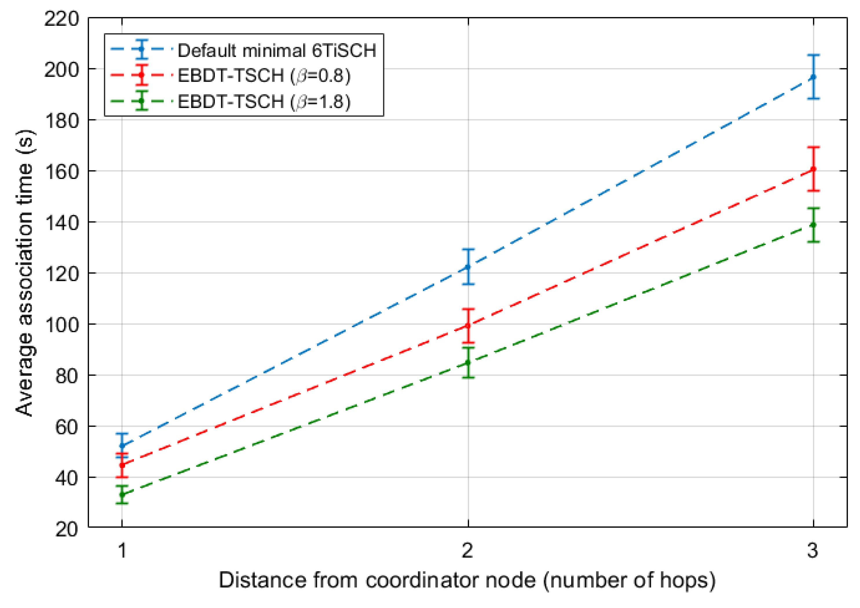
• The proposed mechanism achieves a shorter network formation time than the default association mechanism (i.e., default minimal 6TiSCH configuration) without a relevant increase in implementation complexity.
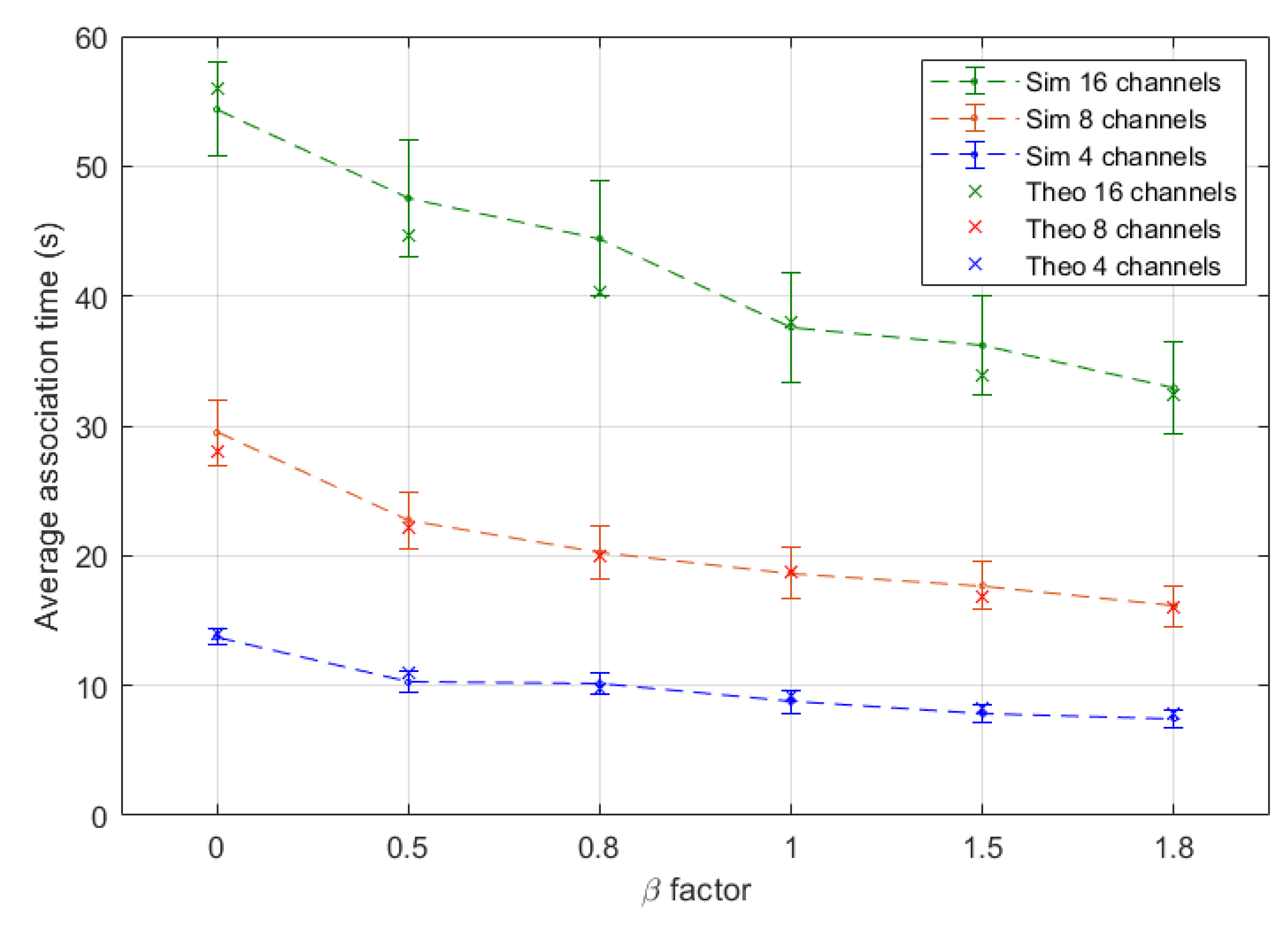
• The proposal is accompanied by a mathematical model validated through simulation, showing a good correspondence between theoretical and simulation results.
• Simulation results demonstrated that the proposed mechanism not only reduces the network formation time, resulting in data packets beginning to be transmitted earlier, but also reduces the energy consumption during the network formation process.

3. TSCH Implementation in Contiki-NG

The IETF IPv6 over the TSCH mode of IEEE 802.15.4e (6TiSCH) working group has standardized protocols to enable low-power, industrial-grade IPv6 networks [25]. 6TiSCH proposes a protocol stack rooted in the TSCH mode of the IEEE 802.15.4-2015 standard, supports multi-hop topologies with routing protocols for low-power and lossy networks (RPL), and is IPv6-ready via 6LoWPAN. 6TiSCH has defined the missing control plane protocols to match link layer resources with the routing topology and the communication needs of the application [26].

The Contiki-NG implementation uses minimal 6TiSCH [27] to define the sublayer for node management and TSCH scheduling. This is described in IETF RFC 8180 [28]. The schedule is outside the scope of the TSCH standard and is not fully covered by 6TiSCH, but does provide a security architecture and simple static programming, including the association process [29]. The IEEE 802.15.4 specification neither defines which EBs are sent nor their content. It is specified that in a minimum TSCH configuration, a node must send an EB within a certain period, which allows a balance between join time and power consumption. Figure 2 illustrates the transmission of EBs in the time domain that a node would carry out to broadcast the presence of the network according to minimal 6TiSCH configuration.

The default minimal 6TiSCH configuration implemented in Contiki-NG establishes a maximum period between transmissions of EBs called $Teb$. The time between the ${(j-1)}^{th}$ and $j^{th}$ EB, denoted $Tebj$, follows a uniform distribution, such that $Tebj\sim U(T_{min},Teb)$, where $T_{min}$ is typically defined as a fraction of $Teb$ (e.g., $0.75Teb$). $Teb$ can be previously defined and remains unchanged during execution. This minimal mode of operation uses a single slotframe. The TSCH slotframe is composed of an adjustable number of time slots and its structure is advertised in the EB, influencing power consumption. The way to adjust it is outside the scope of RFC 8180, but it is implemented in Contiki-NG. RFC 8180 states that there is only one scheduled cell in each slotframe.

Regarding the scanning algorithm, nodes with the minimum 6TiSCH configuration follow a basic network synchronization method, proposed by IEEE 802.15.4, known as passive TSCH scan (PS-TSCH). In [30], the PS-TSCH algorithm is described in detail. A node seeking to join a TSCH network “listens” for EBs transmitted by an associated (synchronizer or coordinator) node on channels available in the channel hopping sequence. This scan is performed over the sequence in a round-robin way, starting at a random point. Initially, the nodes initialize an index variable, denoted $Ic$, randomly selected between 0 and $m-1$. $Ic$ is used to loop through the hopping sequence and the channels involved during the scanning process. Nodes select a channel from the sequence each time they change the channel being scanned following a round-robin strategy, incrementing $Ic$ by 1 and using the module operation to keep it between 0 and $m-1$. Join-seeker nodes listen on each channel for a configurable period called the $Tchscan$. This time can be configured in the Contiki-NG implementation.

When a join-seeker node receives an EB, it joins the network. It then starts following the defined schedule, which implements RDC by having idle slots in which the radio can sleep to save energy. It sends its EBs to advertise the network and help other nodes to join. EBs can only be sent if there is a previously configured schedule. The increase in EB transmission rate has a positive impact on the reduction of the average association time per node, as well as on the network formation time.

4. Proposed Enhanced Beacons Dynamic Transmission Mechanism

In [31], the contribution consists of a theoretical model to estimate the average time required for a node to associate with a synchronizer. This depends on the available channels and the average number of EBs transmitted until the association is achieved. The theoretical analysis is based on demonstrating that both the channel used by a synchronizer to send the $jth$ EB and the channel being scanned by the join-seeker when the $jth$ EB is sent are independent and identically distributed random variables. Results in [31] show that the average association time depends on m and the average time between EB transmissions. There is a trade-off between the average association time, the time between EB transmissions, and the number of channels used for communication. The use of fewer channels reduces the association time, but also the resilience of the network in the presence of interference. On the other hand, for a fixed number of channels, sending EBs more frequently reduces association time. However, when the association process ends, the frequent EB transmissions cause unnecessary energy consumption in the nodes. Additionally, a high EB transmission rate increases network traffic, which could limit slot availability in the schedule and communications between other network devices in networks with high node density.

This enhanced beacons dynamic transmission over TSCH (EBDT-TSCH) algorithm aims to make dynamic $Teb$ in two phases: the intensive phase and the predetermined phase. The predetermined phase has a transmission period of EBs, upper-bounded by $Teb$ similarly to the 6TiSCH. The intensive phase, on the other hand, presents a period of intensive transmission of EBs in which the maximum time between EBs represents a fraction of $Teb$, so the EBs transmission period in the intensive phase is $Tebi=\alpha Teb$, where $0<\alpha <1$. This algorithm intends to use the intensive phase to decrease the network formation time, whereas the predetermined phase is used to avoid excess power consumption after network formation.

A synchronizer running EBDT-TSCH starts in the intensive phase to associate, in a short time, as many nodes within its reach as possible. As part of the EBDT-TSCH implementation, a threshold parameter (u) delimits the end of the intensive phase and the beginning of the predetermined phase. The u parameter constitutes the number of EBs that will be sent during the intensive phase and is computed as $u=\lfloor \beta m\rfloor$, whereas the previously discussed m is the number of available network channels and $\beta \in \Re ,\beta ⩾0$. After u EBs have been sent, the predetermined phase begins, in which the synchronizer reconfigures the maximum EB transmission period to $Teb$. Let us denote $t_i\sim U(\rho Tebi,Tebi)$ and $t_p\sim U(\rho Teb,Teb)$$0<\rho <1$, as the time between successive EB transmission in the intensive phase and the predetermined phase, respectively. Algorithm 1 shows the steps to be followed by a synchronizing node that implements EBDT-TSCH.

Figure 3 illustrates an example of the timeline of EB transmissions performed by a synchronizing node following the EBDT-TSCH algorithm. In this example, $m=4$, $\alpha =0.5$, $\rho =0.75$, and $\beta =1$ are considered. In this way, four EBs are sent ($u=4$) in the intensive phase, and the time between them ($t_i$) follows a uniform distribution and maximum period equal to $Tebi=0.5Teb$. After that, the predetermined phase starts, and the time between successive EBs is also uniformly distributed, but with maximum value $Teb$.

The proposed EBDT-TSCH does not imply a significant increase in implementation complexity and can be used in any network that uses the TSCH association mechanism. Achieving rapid association is particularly important in TSCH-based solutions that consider mobility in the network nodes. The proposed EBDT-TSCH mechanism can be used in conjunction with the proposals presented in [32,33,34] to accelerate the network formation process and to improve mobility management. Variants of TSCH have also been proposed to expand its use in long-range networks such as LoRa [35,36]. In these scenarios, the proposed EBDT-TSCH mechanism can also be used.

Algorithm 1 EBDT-TSCH

Input: $\alpha$, $\beta$, $\rho$, $Teb$ $Tebi\leftarrow \alpha Teb$ $u\leftarrow \lfloor \beta m\rfloor$ $j=0$ while$true$do     if $j<u$ then         $EB\_Period\leftarrow U(\rho Tebi,Tebi)$     else         $EB\_Period\leftarrow U(\rho Teb,Teb)$     end if     $j=j+1$      send EB using $EB\_Period$ end while

4.1. Theoretical Network Formation Expected Time

The analytical model developed in [31] proves that in a network with m channels, the probability for a join-seeker to get associated with a synchronizer after exactly j EB transmissions can be computed following [31] (Equation (5)):

$$P_j=P_n{(1-P_n)}^{j-1},$$

(2)

where $P_n=m^{-1}$ is the probability of the synchronizer sending an EB on the channel scanned by the join-seeker.

In the following, we develop an analytical model for the proposed EBDT-TSCH (the code used to validate the mathematical model as well as to obtain the figures associated with it is available at https://github.com/erikortiz84/EBDT-TSCH.git). The maximum time between successive EBs changes dynamically in EBDT-TSCH. In the intensive phase ($j\le u$), the average elapsed time to send the j EBs is $jE\left(t_i\right)$. Meanwhile, in the predetermined phase, the average elapsed time to send j EBs, $j>u$ EB can be computed as the time needed to send the first u EBs plus the time to send the rest of the $j-u$ EBs. Therefore, we can formalize the average elapsed time to send the $j^{th}$ EB at any phase as the following:

$$E\left(t_j\right)=\left\{\begin{array}{cc}jE\left(t_i\right),\hfill & j\le u\hfill \\ uE\left(t_i\right)+(j-u)E\left(t_p\right),\hfill & j>u,\hfill \end{array}\right.$$

(3)

where $E\left(x\right)$ is the expected value of x. As both, $t_i$ and $t_p$ follow a uniform distribution:

$$E\left(t_i\right)={\displaystyle \frac{\rho +1}{2}}Tebi;$$

(4)

$$E\left(t_p\right)={\displaystyle \frac{\rho +1}{2}}Teb.$$

(5)

Using (2), (3), and the expected value definition, we derive the average time needed for a join-seeker to get associated with a synchronizer as the following:

$$\begin{array}{cc}\hfill E\left(t\right)& =\sum _{j=1}^{\infty }{P}_{j}E\left(t_j\right),\hfill \\ \hfill & =\sum _{j=1}^u{P}_n{(1-P_n)}^{j-1}jE\left(t_i\right)+\sum _{j=u+1}^{\infty }{P}_n{(1-P_n)}^{j-1}\left(uE\left(t_i\right)+(j-u)E\left(t_p\right)\right).\hfill \end{array}$$

(6)

Working on (6) and using (4) and (5) for the proposed EBDT-TSCH, the expected time needed for a join-seeker to get associated with the network is as follows (see proof in Appendix A):

$$E\left(t\right)={\displaystyle \frac{Teb(1+\rho )m}{2}}\left(\alpha -(\alpha -1){\left(1-{\displaystyle \frac{1}{m}}\right)}^{\lfloor \beta m\rfloor }\right).$$

(7)

4.2. EBDT-TSCH Configuration Parameters

The configuration parameters of EBDT-TSCH (i.e., $\alpha$ and $\beta$) and the theoretical expected time for a join-seeker to get associated to a synchronizer ($E\left(t\right)$) are shown in Figure 4. Greater $\alpha$ values reduce the differences in the maximum time between successive EB transmissions in the intensive and predetermined phases, reducing the positive impact of using the proposed EBDT-TSCH. When $\beta$ increases, the number of EB transmissions in the intensive phase also increases, increasing the probability of getting associated in the intensive phase and reducing the average elapsed time to get associated. However, after certain values of $\beta$, the impact in the elapsed association time decreases.

Using (2), we derive the probability of getting associated during the intensive phase as the following:

$$P_{intensive}=\sum _{j=1}^u{P}_n{(1-P_n)}^{j-1},$$

(8)

working in (8) and substituting $u=\lfloor \beta m\rfloor$ and $P_n=m^{-1}$, $P_{intensive}$ can be rewritten as follows:

$$P_{intensive}=1-{\left({\displaystyle \frac{m-1}{m}}\right)}^{\lfloor \beta m\rfloor }.$$

(9)

Figure 5 shows the impact of $\beta$ on the probability of getting associated at the intensive phase given by (9). Smaller $\beta$ values reduce the impact of the intensive phase because the probability of joining at this phase becomes low. On the other hand, there is no incentive to make $\beta >2.8$ because the joining probability at the intensive phase does not increase significantly, causing an increase in the number of EBs transmitted without a relevant reduction in the elapsed time to get associated. The probability of getting associated at the intensive phase in the range of 0.75–0.95 offers a good trade-off between the number of EBs transmitted and the probability of getting associated at the intensive phase; therefore, $\beta$ must be in the range 1.4–2.8 to fulfill this requirement.

5. Experimental Results and Discussion

To assess the performance of the proposed method, comparisons are made by performing multiple simulations. For this purpose, the Cooja simulator, included in the Contiki-NG kernel (The Contiki-NG version used for this research is the Develop v4.0, available at https://github.com/contiki-ng/contiki-ng/tree/develop/v4.0), is used to emulate the communication among Zolertia Z1 nodes. A computer with 16GB of RAM and an Intel Core i7-1185G7 processor was used to run 500 independent simulations, ensuring a maximum mean error of $10\%$ for a $95\%$ confidence interval. Three different scenarios are used to evaluate the performance of the proposed EBDT-TSCH. The parameters used in the simulation are shown in

Table 1. Simulation parameters.

Parameter	Symbol	Value/Calculation
Slotframe length	L	11 slots
Number of network channels	m	4, 8, 16
Maximum time between beacons	$Teb$	4 s
Minimum time between beacons	$\rho Teb$	$0.75Teb$
Maximum time between beacons in the intensive phase	$Tebi$	$\alpha Teb$, $\alpha =0.5$
Minimum time between beacons in the intensive phase	$\rho Tebi$	$0.75Tebi$
Number of EBs sent in the intensive phase	u	$\lfloor \beta m\rfloor$, $0\le \beta \le 1.8$
Join-seeker scan period	-	${\displaystyle \frac{Teb-\rho Teb}{2Lm}}$

.

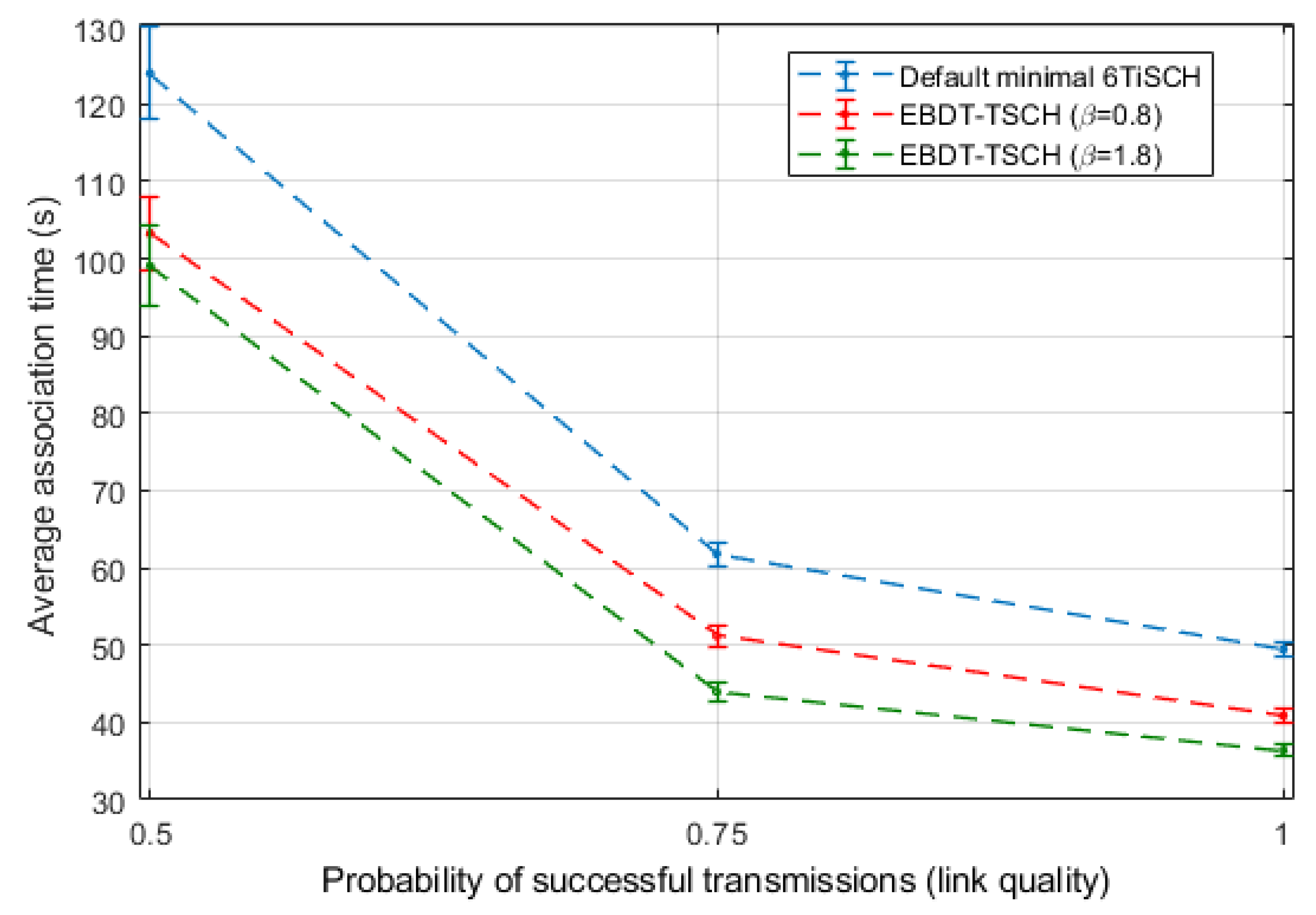
5.1. A Synchronizer–Join-Seeker Pair Scenario

The first scenario is composed of a pair of nodes (a synchronizer and a join-seeker), as shown in Figure 6. The green circle depicts the transmission range of node 1 and the grey circle the interference range. The values of the total number of available channels m and the threshold $u=\lfloor \beta m\rfloor$ that delimits the intensive and the predetermined phases are varied through the simulations.

In this scenario, theoretical results obtained using expression (7) are compared with the simulation results as a function of the number of available channels and $\beta$ values. Figure 7 shows that the theoretical results are inside the confidence interval of the simulation results, thus validating the analytic model developed in Section 4.1. Regardless of the number of available channels, the association time decreases as the $\beta$ factor increases, which implies more transmissions of EBs during the intensive phase. Note that for $\beta =0$ there is no intensive phase, and its results correspond to the behavior of the TSCH with the default minimal 6TiSCH configuration.

There is a trade-off between the number of available network channels, the increase in $\beta$, and the corresponding improvement in the average association time. When there are 16 available network channels, the improvement in the average association time for $\beta =1.8$ versus $\beta =1.5$ is $3.2$ s, but this is only $0.4$ s when 4 channels are compared, for the same values of the $\beta$ factor.

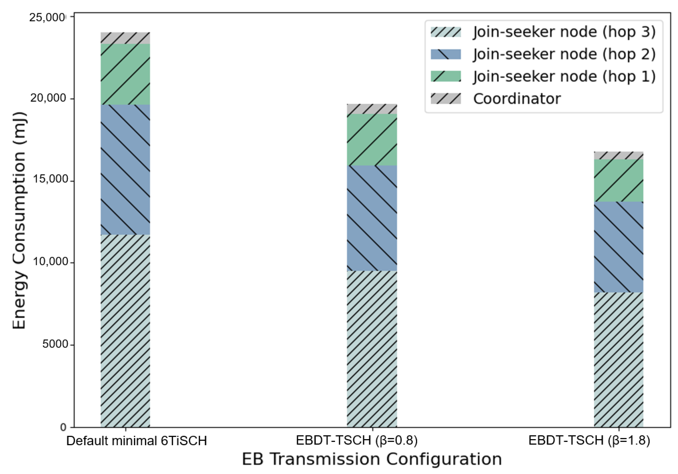
5.2. A Linear Network Scenario

In a second scenario, the behavior of the association process of a linear topology network is evaluated as Figure 8 shows. In this case, the network has a coordinator node and three linearly distributed nodes that seek to associate. The coordinator node’s coverage area is highlighted in green. Each join-seeker node can only listen to EBs generated from its adjacent nodes. In this way, beacons transmitted by node 2 take one hop to reach the coordinator, whereas beacons transmitted by node 4 need to take three hops to reach the coordinator. From now on, the number of hops necessary to reach the coordinator will be called the distance from the coordinator node.

To evaluate the impact of EBDT-TSCH in linear networks, a comparison is made using the default method in Contiki-NG, which follows the 6TiSCH minimal configuration. Figure 9 shows the average association time as a function of distance to coordinator node for three configurations being EBDT-TSCH with $\beta =0.8$, EBDT-TSCH $\beta =1.8$, and default minimal 6TiSCH. The number of available channels is set to 16 and $Teb$ is set to 4 s.

As shown in Figure 9, the average association time increases linearly as the network depth increases. The results show a reduction in the association time between nodes with the proposed EBDT-TSCH mechanism, compared to the default 6TiSCH minimal configuration. The implementation of the proposed algorithm decreases the average association time of the node located three hops away from the coordinator by $18.33\%$ and $29.46\%$ for $\beta =0.8$ and $\beta =1.8$, respectively, compared to the results obtained with minimal 6TiSCH default implementation.

The improvement provided by EBDT-TSCH allows for faster network formation, which results in earlier data packet transmission. The decrease in network formation time is also reflected in energy consumption during network formation. This can be observed in Figure 10, which shows the energy consumption of the network, which is the sum of the average energy consumption of each node during network formation. It is lower for the proposed method when compared with default implementation of minimal 6TiSCH, reducing it up to 18.25% and 30.16% for $\beta =0.8$ and $\beta =1.8$, respectively.

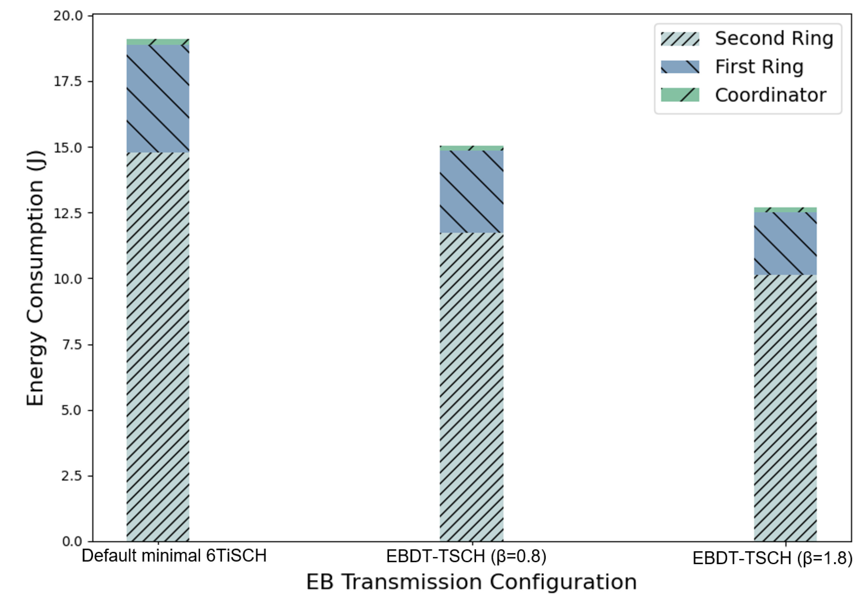
5.3. A Ring Network Scenario

To have a closer look at the network topologies implemented in the real scenarios, simulations of scenarios where the nodes belonging to the network are distributed in the form of rings are also presented. The join-seekers are deployed forming rings around the coordinator node, which acts as a sink as shown in Figure 11. In addition, the link quality is also considered to provide the simulations with a metric that allows the representation of deficiencies in the communication channel. The link quality parameter indicates the probability of successful transmissions.

The scenario displays two rings of nodes, accumulating ten join-seekers and one coordinator node. As in the previous case, a comparison is made between the same three different configurations, $Teb=4$ s, and a total of 4 available channels are set. Figure 12 shows the average network association time.

Also in this scenario, the network performance under the implementation of EBDT-TSCH improves the behavior obtained by default minimal 6TiSCH during the network formation process despite the link quality between nodes. For example, in the scenario that has $0.75$ probability of successful transmission, the configurations of EBDT-TSCH with $\beta =0.8$ and $\beta =1.8$ manage to reduce the average network formation time obtained by 6TiSCH by $17.20\%$ and $28.77\%$, respectively.

Figure 13 shows the average energy consumption during network formation corresponding to the scenario whose link quality value is $0.75$. The consumption generated by the network is shown, composed of the contribution of each ring of join-seekers and the coordinator. The contribution of each ring is estimated as the sum of the average energy consumption of each join-seeker node of the ring. The simulation results show that the EBDT-TSCH configurations decrease energy consumption obtained by the default minimal 6TiSCH configuration by $21.27$% for $\beta =0.8$ and $33.65$% for $\beta =1.8$, respectively.

6. Conclusions and Future Work

The minimal 6TiSCH configuration describes the association mechanism for TSCH through the periodic sending of enhanced beacons. The configuration of the time between beacons has a direct impact on the network formation time. The shorter the time between beacons, the less time necessary for a node to associate with the network and consequently the less time it will take for the network formation. Reducing the time required for a node to associate with the network guarantees that data packet transmission can start earlier. On the other hand, permanently reducing the time between beacons also implies an increase in traffic and energy consumption for the devices.

The EBDT-TSCH mechanism proposed in this work performs dynamic management of the time between EB transmissions that permits starting with a high EB transmission rate to shorten the average time necessary for the nodes to get associated. After the intensive phase, during which all or most of the nodes could associate, the EB transmission rate is decreased to avoid unnecessary energy consumption.

Both the theoretical model and simulation results confirm the effectiveness of the proposed approach. In scenarios where communication between nodes may fail due to channel conditions, the EBDT-TSCH mechanism also demonstrated a reduction in network formation time and energy consumption required for association compared to the minimal 6TiSCH configuration. The implementation of EBDT-TSCH is a simple solution that does not imply a high implementation cost and can be used in any application that uses the association mechanism proposed by 6TiSCH.

A future extension of our work aims to combine the proposed mechanism with the information extracted from the routing protocol to optimize the duration of the intensive phase. We also intend to evaluate the performance of the proposed mechanism in scenarios with greater node density and consider mobile nodes to determine the impact of our proposal on the performance of the handover mechanisms.

References

1. Shafique, K.; Khawaja, B.A.; Sabir, F.; Qazi, S.; Mustaqim, M. Internet of Things (IoT) for Next-Generation Smart Systems: A Review of Current Challenges, Future Trends and Prospects for Emerging 5G-IoT Scenarios. IEEE Access 2020, 8, 23022–23040. [Google Scholar] [CrossRef]
2. Li, X.; Xu, L.D. A Review of Internet of Things—Resource Allocation. IEEE Internet Things J. 2021, 8, 8657–8666. [Google Scholar] [CrossRef]
3. Ud Din, I.; Guizani, M.; Hassan, S.; Kim, B.S.; Khurram Khan, M.; Atiquzzaman, M.; Ahmed, S.H. The Internet of Things: A Review of Enabled Technologies and Future Challenges. IEEE Access 2019, 7, 7606–7640. [Google Scholar] [CrossRef]
4. Kandris, D.; Nakas, C.; Vomvas, D.; Koulouras, G. Applications of Wireless Sensor Networks: An Up-to-Date Survey. Appl. Syst. Innov. 2020, 3, 14. [Google Scholar] [CrossRef]
5. 802.15.4c-2009; IEEE Standard for Information Technology, Part 15.4: Wireless Medium Access Control (MAC) and Physical Layer (PHY) Specifications for Low-Rate Wireless Personal Area Networks (LRWPANS). IEEE: Piscataway, NJ, USA, 2009. [CrossRef]
6. De Guglielmo, D.; Brienza, S.; Anastasi, G. IEEE 802.15.4e: A survey. Comput. Commun. 2016, 88, 1–24. [Google Scholar] [CrossRef]
7. Mantilla Gonzalez, I.A.; Meyer, F.; Turau, V. A Comprehensive Performance Comparison of IEEE 802.15.4 DSME and TSCH in a Realistic IoT Scenario for Industrial Applications. ACM Trans. Internet Things 2023, 4, 1–30. [Google Scholar] [CrossRef]
8. Vera-Pérez, J.; Silvestre-Blanes, J.; Sempere-Payá, V. TSCH and RPL Joining Time Model for Industrial Wireless Sensor Networks. Sensors 2021, 21, 3904. [Google Scholar] [CrossRef] [PubMed]
9. Algora, C.M.G.; Lopez, E.P.; Reguera, V.A.; Nowe, A.; Steenhaut, K. Poster: Comparative study of EM-MAC and TSCH/Orchestra for IoT. In Proceedings of the 2016 Symposium on Communications and Vehicular Technologies (SCVT), Mons, Belgium, 22 November 2016; pp. 1–6. [Google Scholar]
10. Raza, S.; van Der Lee, T.; Exarchakos, G.; Güneş, M. A reliability analysis of TSCH protocol in a mobile scenario. In Proceedings of the 2019 16th IEEE Annual Consumer Communications & Networking Conference (CCNC), Las Vegas, NV, USA, 11–14 January 2019; pp. 1–6. [Google Scholar]
11. 802.15.4e-2012; IEEE Standard for Local and Metropolitan Area Networks–Part 15.4: Low-Rate Wireless Personal Area Networks (LR-WPANs) Amendment 1: MAC Sublayer. IEEE: Piscataway, NJ, USA, 2012. [CrossRef]
12. Elsts, A.; Kim, S.; Kim, H.S.; Kim, C. An empirical survey of autonomous scheduling methods for TSCH. IEEE Access 2020, 8, 67147–67165. [Google Scholar] [CrossRef]
13. Vogli, E.; Ribezzo, G.; Grieco, L.A.; Boggia, G. Fast join and synchronization schema in the IEEE 80215.4e MAC. In Proceedings of the 2015 IEEE Wireless Communications and Networking Conference Workshops (WCNCW), New Orleans, LA, USA, 9–12 March 2015; pp. 85–90. [Google Scholar] [CrossRef]
14. Vogli, E.; Ribezzo, G.; Grieco, L.A.; Boggia, G. Fast network joining algorithms in industrial IEEE 802.15.4 deployments. Ad. Hoc. Netw. 2018, 69, 65–75. [Google Scholar] [CrossRef]
15. Duy, T.P.; Kim, Y. An efficient joining scheme in IEEE 80215.4e. In Proceedings of the 2015 International Conference on Information and Communication Technology Convergence (ICTC), Jeju, Republic of Korea, 28–30 October 2015; pp. 226–229. [Google Scholar] [CrossRef]
16. Duy, T.P.; Dinh, T.; Kim, Y. A rapid joining scheme based on fuzzy logic for highly dynamic IEEE 802.15.4e time-slotted channel hopping networks. Int. J. Distrib. Sens. Netw. 2016, 12, 1550147716659424. [Google Scholar] [CrossRef]
17. Kim, J.Y.; Chung, S.H.; Ha, Y.V. A fast joining scheme based on channel quality for IEEE80215.4e TSCH in severe interference environment. In Proceedings of the 2017 Ninth International Conference on Ubiquitous and Future Networks (ICUFN), Milan, Italy, 4–7 July 2017; pp. 427–432. [Google Scholar] [CrossRef]
18. Khoufi, I.; Minet, P.; Livolant, E.; Rmili, B. Building an IEEE 80215.4e TSCH network. In Proceedings of the 2016 IEEE 35th International Performance Computing and Communications Conference (IPCCC), Las Vegas, NV, USA, 9–11 December 2016; pp. 1–2. [Google Scholar] [CrossRef]
19. Khoufi, I.; Minet, P.; Rmili, B. Beacon advertising in an IEEE 802.15.4e TSCH network for space launch vehicles. Acta Astronaut. 2019, 158, 76–88. [Google Scholar] [CrossRef]
20. Vallati, C.; Brienza, S.; Anastasi, G.; Das, S.K. Improving Network Formation in 6TiSCH Networks. IEEE Trans. Mob. Comput. 2019, 18, 98–110. [Google Scholar] [CrossRef]
21. Karalis, A. ATP: A Fast Joining Technique for IEEE80215. 4-TSCH Networks. In Proceedings of the 2018 IEEE 19th International Symposium on “A World of Wireless, Mobile and Multimedia Networks” (WoWMoM), Chania, Greece, 12–15 June 2018; pp. 588–599. [Google Scholar] [CrossRef]
22. Karalis, A.; Zorbas, D.; Douligeris, C. Collision-Free Advertisement Scheduling for IEEE 802.15.4-TSCH Networks. Sensors 2019, 19, 1789. [Google Scholar] [CrossRef] [PubMed]
23. Kalita, A.; Khatua, M. Channel Condition Based Dynamic Beacon Interval for Faster Formation of 6TiSCH Network. IEEE Trans. Mob. Comput. 2021, 20, 2326–2337. [Google Scholar] [CrossRef]
24. Mohamadi, M.; Djamaa, B.; Senouci, M.R.; Mellouk, A. FAN: Fast and Active Network Formation in IEEE 802.15.4 TSCH Networks. J. Netw. Comput. Appl. 2021, 183–184, 103026. [Google Scholar] [CrossRef]
25. 802.15.4w-2020; IEEE Standard for Low-Rate Wireless Networks. IEEE Standard: Piscataway, NJ, USA, 2020. [CrossRef]
26. Vilajosana, X.; Watteyne, T.; Chang, T.; Vučinić, M.; Duquennoy, S.; Thubert, P. Ietf 6tisch: A tutorial. IEEE Commun. Surv. Tutorials 2019, 22, 595–615. [Google Scholar] [CrossRef]
27. Hussain, S.J.; Roopa, M. Performance Assessment of the Minimal 6TiSCH Configuration. In Proceedings of the 2022 International Conference on Computing, Communication, Security and Intelligent Systems (IC3SIS), Communication, Kochi, India, 23–25 June 2022; pp. 1–4. [Google Scholar] [CrossRef]
28. Vilajosana, X.; Pister, K.; Watteyne, T. Minimal IPv6 over the TSCH Mode of IEEE 802.15.4e (6TiSCH) Configuration. 2017. Available online: https://www.rfc-editor.org/info/rfc8180 (accessed on 1 April 2024).
29. Duquennoy, S.; Elsts, A.; Al Nahas, B.; Oikonomo, G. Tsch and 6tisch for contiki: Challenges, design and evaluation. In Proceedings of the 2017 13th International Conference on Distributed Computing in Sensor Systems (DCOSS), Ottawa, ON, Canada, 5–7 June 2017; pp. 11–18. [Google Scholar]
30. Algora, C.M.G.; Reguera, V.A.; Fernández, E.M.G.; Steenhaut, K. Parallel rendezvous-based association for IEEE 802.15. 4 TSCH networks. IEEE Sensors J. 2018, 18, 9005–9020. [Google Scholar] [CrossRef]
31. Algora, C.M.G.; Guerra, E.O.; Montejo-Sánchez, S.; Fernández, E.M.G.; Steenhaut, K. A Theoretical Association Time Model for IEEE 802.15. 4 TSCH Networks. IEEE Commun. Lett. 2020, 25, 656–659. [Google Scholar] [CrossRef]
32. Pettorali, M.; Righetti, F.; Vallati, C.; Das, S.K.; Anastasi, G. Mobility Management in TSCH-based Industrial Wireless Networks. IEEE Trans. Mob. Comput. 2024, 1–18. [Google Scholar] [CrossRef]
33. Tavallaie, O.; Taheri, J.; Zomaya, A.Y. Design and Optimization of Traffic-Aware TSCH Scheduling for Mobile 6TiSCH Networks. In Proceedings of the International Conference on Internet-of-Things Design and Implementation, New York, NY, USA, 18–21 May 2021; IoTDI ’21. pp. 234–246. [Google Scholar] [CrossRef]
34. Pettorali, M.; Righetti, F.; Vallati, C.; Das, S.K.; Anastasi, G. Mobility Management in Industrial IoT Environments. In Proceedings of the 2022 IEEE 23rd International Symposium on a World of Wireless, Mobile and Multimedia Networks (WoWMoM), Belfast, UK, 14–17 June 2022; pp. 271–280. [Google Scholar] [CrossRef]
35. Haubro, M.; Orfanidis, C.; Oikonomou, G.; Fafoutis, X. TSCH-over-LoRA: Long range and reliable IPv6 multi-hop networks for the internet of things. Internet Technol. Lett. 2020, 3, e165. [Google Scholar] [CrossRef]
36. Iglesias-Rivera, A.; Van Glabbeek, R.; Guerra, E.O.; Braeken, A.; Steenhaut, K.; Cruz-Enriquez, H. Time-Slotted Spreading Factor Hopping for Mitigating Blind Spots in LoRa-Based Networks. Sensors 2022, 22, 2253. [Google Scholar] [CrossRef] [PubMed]
Figure 1. Slotframe structure example with parameters: slotframe length 7 slots, s l o t O f f s e t = 3 , and m = 16 available channels.
Futureinternet 16 00187 g001
Figure 2. TSCH linear network association process.
Futureinternet 16 00187 g002
Figure 3. EBDT-TSCH with α = 0.5 , ρ = 0.75 , and β = 1 for 4 available network channels.
Futureinternet 16 00187 g003
Figure 4. Trade-off between α , β , and E ( t ) with m = 16 available channels, T e b = 4 s , and ρ = 0.75 .
Futureinternet 16 00187 g004
Figure 5. Probability of getting associated at the intensive phase for different network available channels, represented by the symbol “x” in discrete values of β .
Futureinternet 16 00187 g005
Figure 6. Pair synchronizer–join-seeker network scenario. Node 1 is the network coordinator and node 2 is a join-seeker. The green circle depicts the transmission range of node 1, while the grey circle depicts the interference range.
Futureinternet 16 00187 g006
Figure 7. EBDT-TSCH association time. Pair synchronizer–join-seeker scenario.
Futureinternet 16 00187 g007
Figure 8. Linear network scenario. The nodes are on a line and each node can only communicate with its adjacent nodes. Node 1 is the network coordinator and nodes 2–4 are join-seekers. The green circle depicts the transmission range of node 1, while the grey circle depicts the interference range.
Futureinternet 16 00187 g008
Figure 9. Association time in a linear network topology.
Futureinternet 16 00187 g009
Figure 10. Average energy consumption of the linear network scenario until all nodes get associated.
Futureinternet 16 00187 g010
Figure 11. Simulation scenario with ring topology. Node 1 is the network coordinator and nodes 2–11 are join-seekers. The green circle depicts the transmission range of node 1, while the grey circle depicts the interference range.
Futureinternet 16 00187 g011
Figure 12. Network formation time in a ring topology for different link quality values.
Futureinternet 16 00187 g012
Figure 13. Average energy consumption of the network in ring topology.
Futureinternet 16 00187 g013