
Metric Space Indices for Dynamic Optimization in a Peer to Peer-Based Image Classification Crowdsourcing Platform

Abstract
1. Introduction
1.1. Research Objectives
1.2. Contribution
1.3. Outline
2. Metric Spaces
3. Previous Work
4. P2P-Based Crowdsourcing Platform
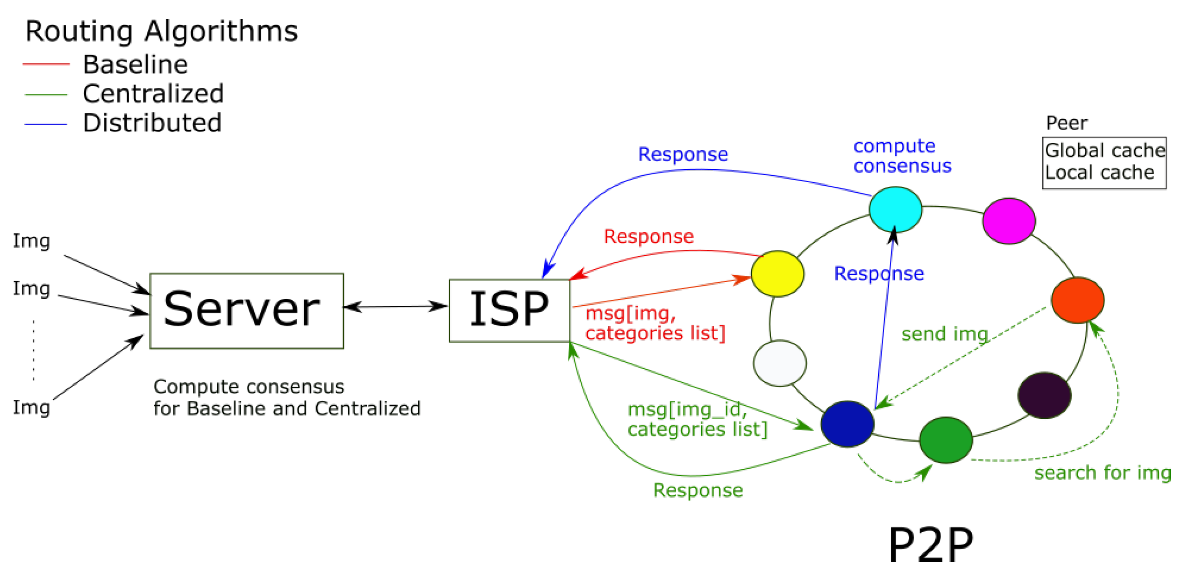
4.1. P2P-Based Platform Architecture
4.2. Routing Algorithms
5. Dynamic Optimization of the Crowdsourcing Platform
5.1. Dynamic Optimization Engine Based on Metric Indices
Building Phase

| Algorithm 1 Algorithm used for the building phase of the dynamic optimization engine. |
|
| Algorithm 2 Algorithm used to build the pivot-based indices. |
|
5.2. Crowdsourcing Platform Parameter Configuration: Scheme of Two Metric Indices
Search Phase
| Algorithm 3 Algorithm used for the search phase of the dynamic optimization engine. |
|
| Algorithm 4 Top-k search algorithm for a pivot-based index. |
|
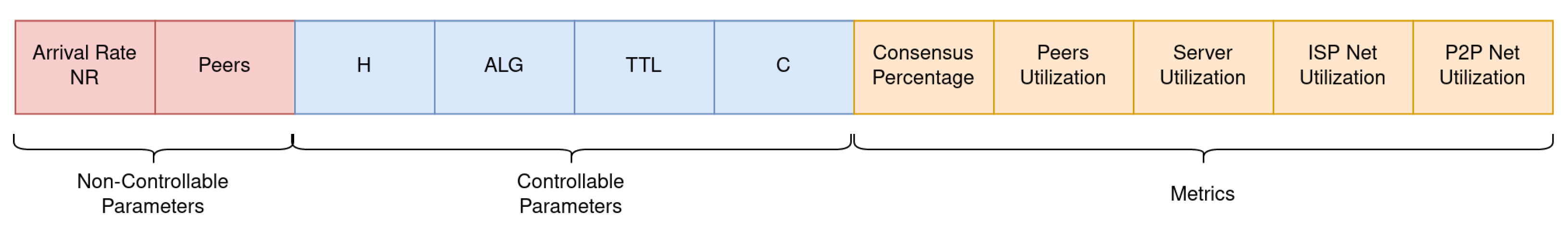
6. Experimental Settings
Alternative Dynamic Optimization Approaches
- IndexLimit: Based on the proposed Index optimization algorithm, but between successive optimization actions the parameter H changes at most 5 units, the parameter can vary 24 units, and the parameter C can vary at most by 5%.
- IndexF: Similar to Index, but during situations without stress, the new configuration vector is applied if the metrics do not match a stress situation.
- Analytic Ad Hoc Controller: This uses Equation (3) to adjust the value of H. This equation is based on the difference between the average utilization of the ISP () and the utilization requested by the data center engineer (e.g., 40%).
- DQL: Deep Q-Learning (DQL) model with Experience Replay, trained with a minimum of 1500 episodes. The model input variables are the same as those presented in Figure 4.
- DQL-O: This is similar to DQL, but we added to the state vector the original values of the controllable parameters set by the data center engineer.
- DQL-Act: We included in the state vector of the model the size of the queue of active tasks on the server. In this way, we evaluated the hypothesis that knowing the number of active tasks can allow the agent to more adequately estimate the server workload.
- DQL-O-Act: This combines the -O and - approaches. The state vector is built with the original values of the controllable parameters and with the size of the list of active tasks of the server.
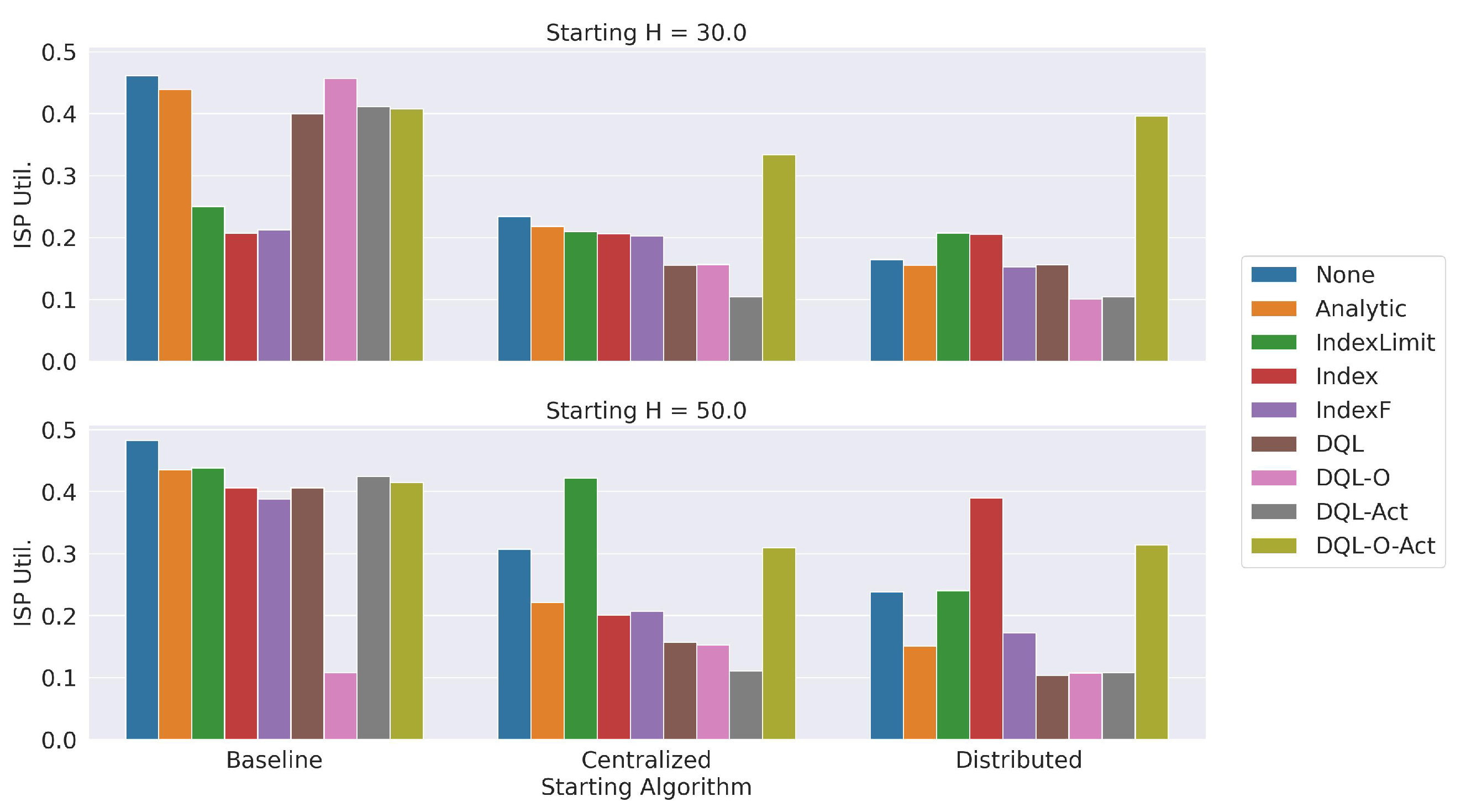
7. Results
7.1. Effectiveness Evaluation
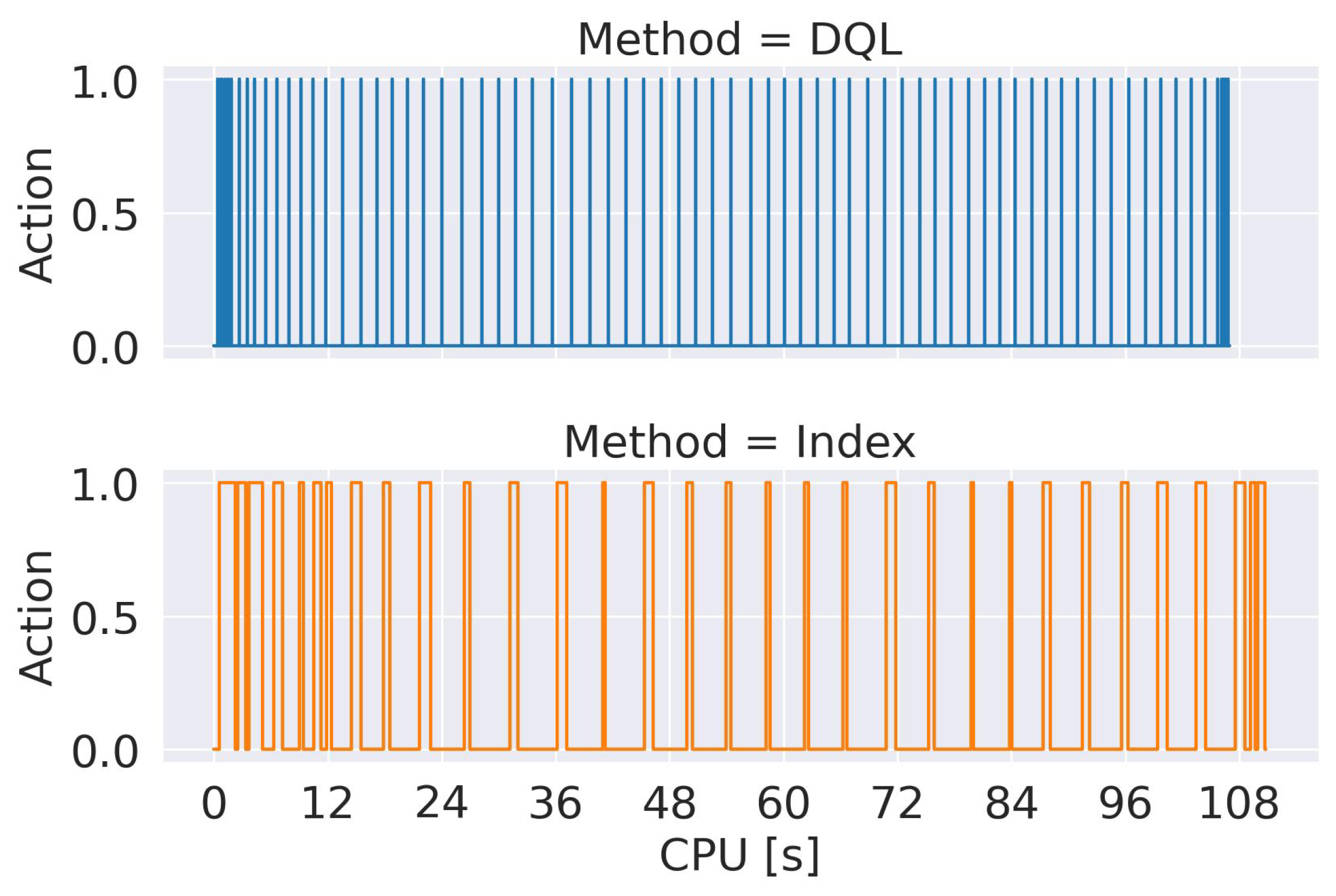
7.2. Execution Time of the Dynamic Optimization Approaches
7.3. Scalability
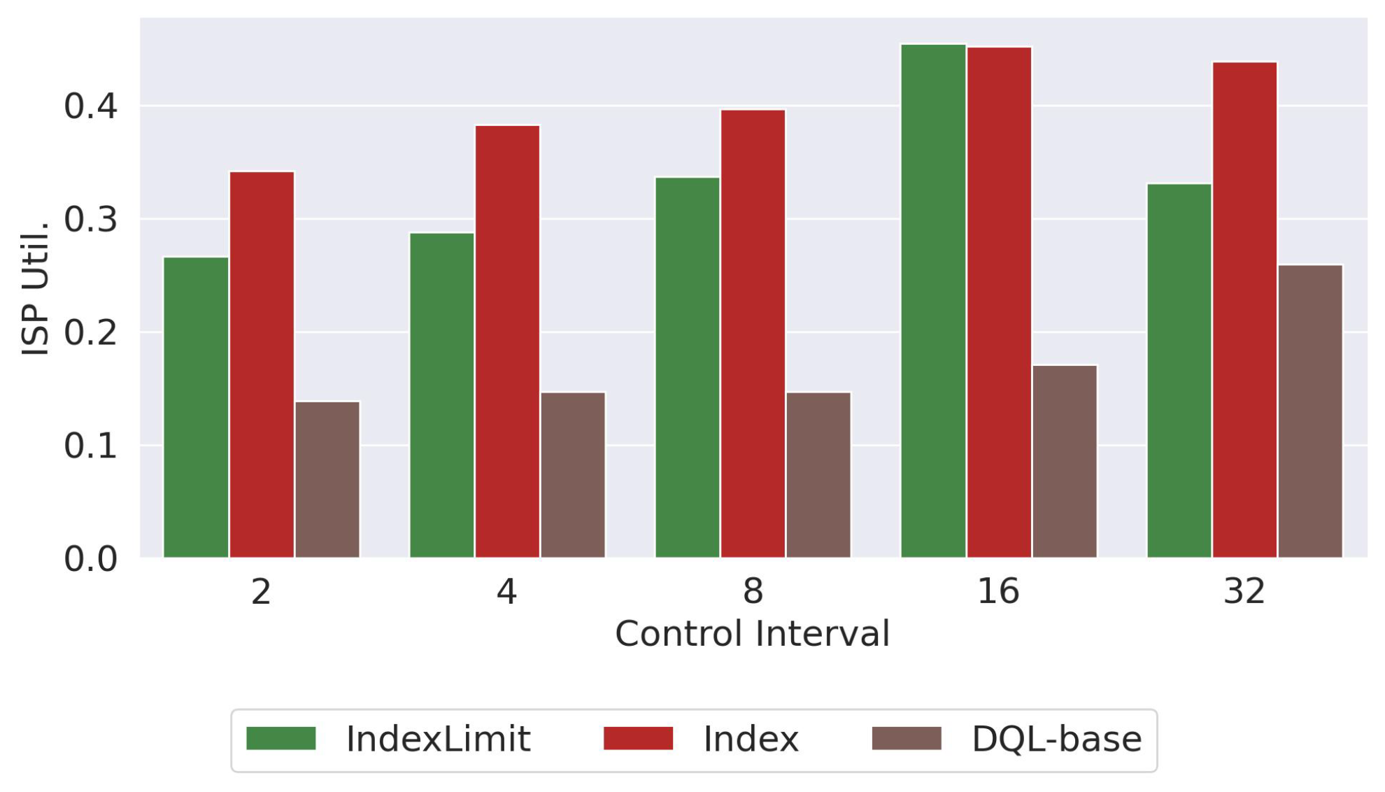
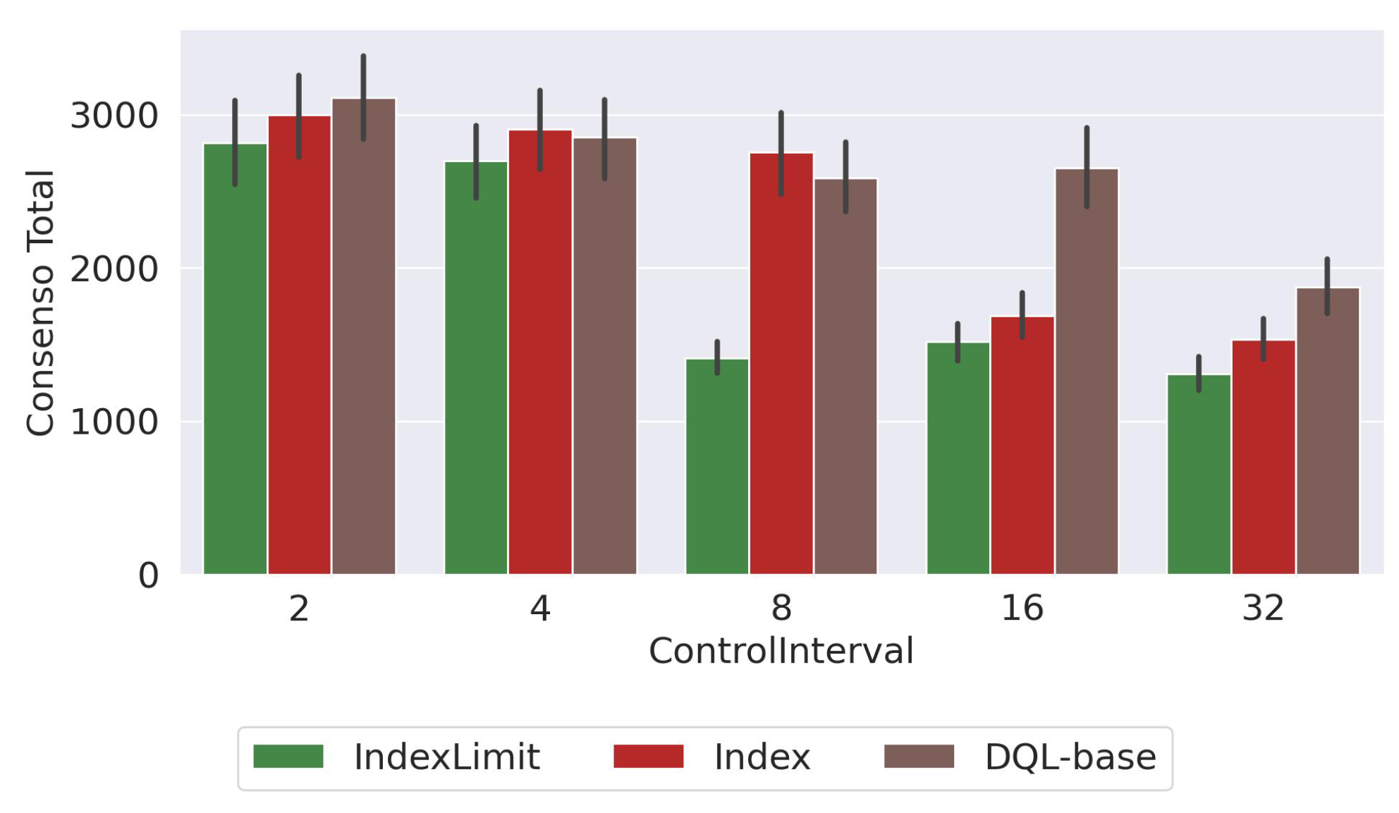
7.4. Size of the Control Window
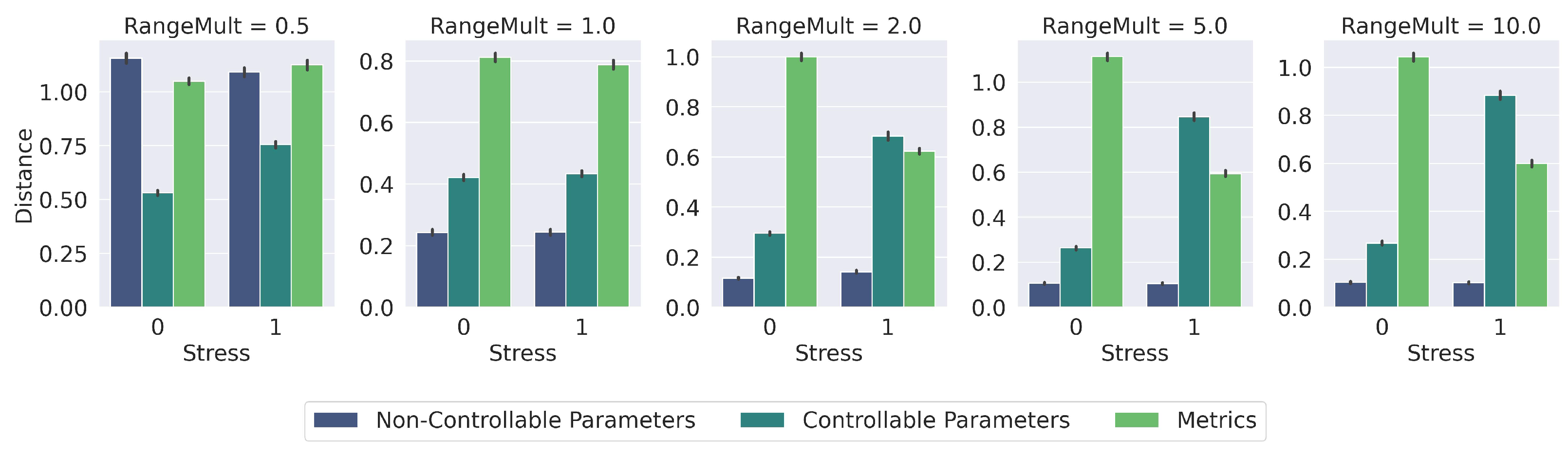
7.4.1. Constants , and
7.4.2. Metric Index Evaluation
8. Conclusions
Author Contributions
Funding
Data Availability Statement
Acknowledgments
Conflicts of Interest
References
- Jamal, A.; Al-Ahmadi, H.M.; Butt, F.M.; Iqbal, M.; Almoshaogeh, M.; Ali, S. Metaheuristics for Traffic Control and Optimization: Current Challenges and Prospects. In Search Algorithm—Essence of Optimization; Harkut, D.D.G., Ed.; IntechOpen: Rijeka, Croatia, 2021; Chapter 2. [Google Scholar] [CrossRef]
- Li, F.; Su, Z.; Wang, G.M. An effective integrated control with intelligent optimization for wastewater treatment process. J. Ind. Inf. Integr. 2021, 24, 100237. [Google Scholar] [CrossRef]
- Song, D.; Liu, J.; Yang, Y.; Yang, J.; Su, M.; Wang, Y.; Gui, N.; Yang, X.; Huang, L.; Hoon Joo, Y. Maximum wind energy extraction of large-scale wind turbines using nonlinear model predictive control via Yin-Yang grey wolf optimization algorithm. Energy 2021, 221, 119866. [Google Scholar] [CrossRef]
- Yazdani, D.; Cheng, R.; Yazdani, D.; Branke, J.; Jin, Y.; Yao, X. A survey of evolutionary continuous dynamic optimization over two decades—Part A. IEEE Trans. Evol. Comput. 2021, 25, 609–629. [Google Scholar] [CrossRef]
- Yazdani, D.; Cheng, R.; Yazdani, D.; Branke, J.; Jin, Y.; Yao, X. A survey of evolutionary continuous dynamic optimization over two decades—Part B. IEEE Trans. Evol. Comput. 2021, 25, 630–650. [Google Scholar] [CrossRef]
- Wang, P.; Qin, J.; Li, J.; Wu, M.; Zhou, S.; Feng, L. Dynamic Optimization Method of Wireless Network Routing Based on Deep Learning Strategy. Mob. Inf. Syst. 2022, 2022. [Google Scholar] [CrossRef]
- Tuli, S.; Poojara, S.R.; Srirama, S.N.; Casale, G.; Jennings, N.R. COSCO: Container Orchestration Using Co-Simulation and Gradient Based Optimization for Fog Computing Environments. IEEE Trans. Parallel Distrib. Syst. 2022, 33, 101–116. [Google Scholar] [CrossRef]
- Karthick, T.; Charles Raja, S.; Jeslin Drusila Nesamalar, J.; Chandrasekaran, K. Design of IoT based smart compact energy meter for monitoring and controlling the usage of energy and power quality issues with demand side management for a commercial building. Sustain. Energy Grids Netw. 2021, 26, 100454. [Google Scholar]
- Marín, M.; Gil-Costa, V.; Inostrosa-Psijas, A.; Bonacic, C. Hybrid capacity planning methodology for web search engines. Simul. Model. Pract. Theory 2019, 93, 148–163. [Google Scholar] [CrossRef]
- Gosavi, A. Simulation-Based Optimization; Springer: Berlin/Heidelberg, Germany, 2015. [Google Scholar]
- Shi, Y.; Sagduyu, Y.E.; Erpek, T. Reinforcement learning for dynamic resource optimization in 5G radio access network slicing. In Proceedings of the 2020 IEEE 25th International Workshop on Computer Aided Modeling and Design of Communication Links and Networks (CAMAD), Pisa, Italy, 14–16 September 2020; IEEE: Piscataway, NJ, USA, 2020; pp. 1–6. [Google Scholar]
- Mosavi, A.; Faghan, Y.; Ghamisi, P.; Duan, P.; Ardabili, S.F.; Salwana, E.; Band, S.S. Comprehensive review of deep reinforcement learning methods and applications in economics. Mathematics 2020, 8, 1640. [Google Scholar] [CrossRef]
- Loor, F.; Manriquez, M.; Gil-Costa, V.; Marín, M. Feasibility of P2P-STB based crowdsourcing to speed-up photo classification for natural disasters. Clust. Comput. 2022, 25, 279–302. [Google Scholar] [CrossRef]
- Chávez, E.; Navarro, G.; Baeza-Yates, R.; Marroquín, J.L. Searching in metric spaces. ACM Comput. Surv. 2001, 33, 273–321. [Google Scholar] [CrossRef]
- Bebis, G. Fingerprint Indexing. In Encyclopedia of Biometrics; Li, S.Z., Jain, A., Eds.; Springer: Boston, MA, USA, 2009; pp. 491–496. [Google Scholar] [CrossRef]
- Gil-Costa, V.; Santos, R.L.; Macdonald, C.; Ounis, I. Modelling efficient novelty-based search result diversification in metric spaces. J. Discret. Algorithms 2013, 18, 75–88. [Google Scholar] [CrossRef]
- Echihabi, K.; Zoumpatianos, K.; Palpanas, T. High-dimensional similarity search for scalable data science. In Proceedings of the 2021 IEEE 37th International Conference on Data Engineering (ICDE), Chania, Greece, 19–22 April 2021; IEEE: Piscataway, NJ, USA, 2021; pp. 2369–2372. [Google Scholar]
- Zezula, P.; Amato, G.; Dohnal, V.; Batko, M. Similarity Search: The Metric Space Approach; Advances in Database Systems; Springer: New York, NY, USA, 2006; Volume 32. [Google Scholar]
- Samet, H. Foundations of Multidimensional and Metric Data Structures (The Morgan Kaufmann Series in Computer Graphics and Geometric Modeling); Morgan Kaufmann Publishers Inc.: Burlington, MA, USA, 2005. [Google Scholar]
- Mamede, M.; Barbosa, F. Range queries in natural language dictionaries with recursive lists of clusters. In Proceedings of the 22nd International Symposium on Computer and Information Sciences, ISCIS, Ankara, Turkey, 7–9 November 2007. [Google Scholar]
- Baeza-Yates, R.; Cunto, W.; Manber, U.; Wu, S. Proximity Matching Using Fixed-Queries Trees. In Proceedings of the 5th Annual Symposium on Combinatorial Pattern Matching, CPM, LNCS 807, Asilomar, CA, USA, 5–8 June 1994; pp. 198–212. [Google Scholar]
- Mico, L.; Oncina, J.; Vidal, E. A new version of the nearest-neighbor approximating and eliminating search (AESA) with linear preprocessing-time and memory requirements. Pattern Recogn. Lett. 1994, 15, 9–17. [Google Scholar] [CrossRef]
- Gennaro, C.; Mordacchini, M.; Orlando, S.; Rabitti, F. A Scalable Distributed Data Structure for Multi-Feature Similarity Search. In Proceedings of the Sixteenth Italian Symposium on Advanced Database Systems, SEBD, Mondello, PA, Italy, 22–25 June 2008; pp. 302–309. [Google Scholar]
- Chen, L.; Gao, Y.; Zheng, B.; Jensen, C.S.; Yang, H.; Yang, K. Pivot-based metric indexing. In Proceedings of the VLDB Endowment: 43rd International Conference, Munich, Germany, 28 August–1 September 2017. [Google Scholar]
- Gil-Costa, V.; Marin, M.; Reyes, N. Parallel query processing on distributed clustering indexes. J. Discret. Algorithms 2009, 7, 3–17. [Google Scholar] [CrossRef]
- Argentina, S.; Quinteros, A.; García, R.H.; Frati, F.E.; Barrientos, R.J. A Comparative Analysis of Massive Finger-Vein Recognition Algorithms: From Energy Consumption Perspective. In Proceedings of the 2022 41st International Conference of the Chilean Computer Science Society (SCCC), Santiago, Chile, 21–25 November 2022; pp. 1–6. [Google Scholar]
- Artigas-Fuentes, F.J.; Badía, J.M. Accessing very high dimensional spaces in parallel. J. Supercomput. 2017, 73, 176–189. [Google Scholar] [CrossRef]
- Safaee, S.; Mirabi, M.; Safaei, A.A. StreamFilter: A framework for distributed processing of range queries over streaming data with fine-grained access control. Clust. Comput. 2024, 73, 1573–7543. [Google Scholar] [CrossRef]
- Novak, D.; Batko, M.; Zezula, P. Large-scale similarity data management with distributed Metric Index. Inf. Process. Manag. 2012, 48, 855–872. [Google Scholar] [CrossRef]
- Catalyurek, U.V.; Boman, E.G.; Devine, K.D.; Bozdağ, D.; Heaphy, R.T.; Riesen, L.A. A repartitioning hypergraph model for dynamic load balancing. Parallel Distrib. Comput. 2009, 69, 711–724. [Google Scholar] [CrossRef]
- Yang, K.; Ding, X.; Zhang, Y.; Chen, L.; Zheng, B.; Gao, Y. Distributed similarity queries in metric spaces. Data Sci. Eng. 2019, 4, 93–108. [Google Scholar] [CrossRef]
- Gadaleta, M.; Chiariotti, F.; Rossi, M.; Zanella, A. D-DASH: A deep Q-learning framework for DASH video streaming. IEEE Trans. Cogn. Commun. Netw. 2017, 3, 703–718. [Google Scholar] [CrossRef]
- Ding, D.; Fan, X.; Zhao, Y.; Kang, K.; Yin, Q.; Zeng, J. Q-learning based dynamic task scheduling for energy-efficient cloud computing. Future Gener. Comput. Syst. 2020, 108, 361–371. [Google Scholar] [CrossRef]
- Luong, N.C.; Hoang, D.T.; Gong, S.; Niyato, D.; Wang, P.; Liang, Y.C.; Kim, D.I. Applications of deep reinforcement learning in communications and networking: A survey. IEEE Commun. Surv. Tutor. 2019, 21, 3133–3174. [Google Scholar] [CrossRef]
- Wang, L.; Pan, Z.; Wang, J. A review of reinforcement learning based intelligent optimization for manufacturing scheduling. Complex Syst. Model. Simul. 2021, 1, 257–270. [Google Scholar] [CrossRef]
- Yang, H.; Li, W.; Wang, B. Joint optimization of preventive maintenance and production scheduling for multi-state production systems based on reinforcement learning. Reliab. Eng. Syst. Saf. 2021, 214, 107713. [Google Scholar] [CrossRef]
- Rabault, J.; Ren, F.; Zhang, W.; Tang, H.; Xu, H. Deep reinforcement learning in fluid mechanics: A promising method for both active flow control and shape optimization. J. Hydrodyn. 2020, 32, 234–246. [Google Scholar] [CrossRef]
- Yu, C.; Liu, J.; Nemati, S.; Yin, G. Reinforcement learning in healthcare: A survey. ACM Comput. Surv. (CSUR) 2021, 55, 1–36. [Google Scholar] [CrossRef]
- Kompella, V.; Capobianco, R.; Jong, S.; Browne, J.; Fox, S.; Meyers, L.; Wurman, P.; Stone, P. Reinforcement learning for optimization of COVID-19 mitigation policies. arXiv 2020, arXiv:2010.10560. [Google Scholar]
- Boulesnane, A.; Meshoul, S. Reinforcement learning for dynamic optimization problems. In Proceedings of the Genetic and Evolutionary Computation Conference Companion, Lille, France, 10–14 July 2021; pp. 201–202. [Google Scholar]
- Forootani, A.; Zarch, M.G.; Tipaldi, M.; Iervolino, R. A stochastic dynamic programming approach for the machine replacement problem. Eng. Appl. Artif. Intell. 2023, 118, 105638. [Google Scholar] [CrossRef]
- Rowstron, A.; Druschel, P. Pastry: Scalable, Decentralized Object Location, and Routing for Large-Scale Peer-to-Peer Systems. In Proceedings of the Middleware 2011, Lisbon, Portugal, 12–16 December 2011; Guerraoui, R., Ed.; Springer: Berlin/Heidelberg, Germany, 2001; pp. 329–350. [Google Scholar]
- Corradi, A.; Fanelli, M.; Foschini, L. VM consolidation: A real case based on OpenStack Cloud. Future Gener. Comput. Syst. 2014, 32, 118–127. [Google Scholar] [CrossRef]
- Marzolla, M. Libcppsim: A Simula-like, portable process-oriented simulation library in C++. In Proceedings of the 18th European Simulation Multiconference, ESM’04, Magdeburg, Germany, 13–16 June 2004; pp. 222–227. [Google Scholar]
- Xia, G.S.; Bai, X.; Ding, J.; Zhu, Z.; Belongie, S.; Luo, J.; Datcu, M.; Pelillo, M.; Zhang, L. DOTA: A Large-Scale Dataset for Object Detection in Aerial Images. In Proceedings of the IEEE Conference on Computer Vision and Pattern Recognition (CVPR), Salt Lake City, UT, USA, 18–23 June 2018. [Google Scholar]
- Cheng, G.; Han, J. A survey on object detection in optical remote sensing images. ISPRS J. Photogramm. Remote Sens. 2016, 117, 11–28. [Google Scholar] [CrossRef]
- Alam, F.; Ofli, F.; Imran, M. Crisismmd: Multimodal twitter datasets from natural disasters. In Proceedings of the Twelfth International AAAI Conference on Web and Social Media, Palo Alto, CA, USA, 25–28 June 2018. [Google Scholar]
- Bhavaraju, S.K.T.; Beyney, C.; Nicholson, C. Quantitative analysis of social media sensitivity to natural disasters. Int. J. Disaster Risk Reduct. 2019, 39, 101251. [Google Scholar] [CrossRef]
- Imran, M.; Mitra, P.; Castillo, C. Twitter as a lifeline: Human-annotated twitter corpora for NLP of crisis-related messages. arXiv 2016, arXiv:1605.05894. [Google Scholar]
- Kurkcu, A.; Zuo, F.; Gao, J.; Morgul, E.F.; Ozbay, K. Crowdsourcing incident information for disaster response using twitter. In Proceedings of the Transportation Research Board 96th Annual Meeting, Washington, DC, USA, 8–12 January 2017; pp. 1–17. [Google Scholar]
- Murthy, D.; Gross, A.J. Social media processes in disasters: Implications of emergent technology use. Soc. Sci. Res. 2017, 63, 356–370. [Google Scholar] [CrossRef] [PubMed]
- Danylo, O.; Moorthy, I.; Sturn, T.; See, L.; Laso Bayas, J.C.; Domian, D.; Fraisl, D.; Giovando, C.; Girardot, B.; Kapur, R.; et al. The Picture Pile tool for rapid image assessment: A demonstration using Hurricane Matthew. ISPRS Ann. Photogramm. Remote Sens. Spat. Inf. Sci. 2018, 4, 27–32. [Google Scholar] [CrossRef]
- Rogstadius, J.; Vukovic, M.; Teixeira, C.A.; Kostakos, V.; Karapanos, E.; Laredo, J.A. CrisisTracker: Crowdsourced social media curation for disaster awareness. IBM J. Res. Dev. 2013, 57, 4:1–4:13. [Google Scholar] [CrossRef]
- Salk, C.F.; Sturn, T.; See, L.; Fritz, S. Limitations of majority agreement in crowdsourced image interpretation. Trans. GIS 2017, 21, 207–223. [Google Scholar] [CrossRef]
- Falcão, I.W.; Seruffo, M.C.; Souza, D.D.S.; Cardoso, D.L.; Ferreira, J.J.; Da Silva, M.S. A Comparative Analysis of Local and Cloud Access Assessment for Multimodal Interactive Application. In Proceedings of the 2018 4th International Conference on Cloud Computing Technologies and Applications, Cloudtech Brussels, Belgium, 26–28 November 2018. [Google Scholar]
- Qarout, R.K.; Checco, A.; Bontcheva, K. Investigating stability and reliability of crowdsourcing output. In Proceedings of the CEUR Workshop Proceedings, Zürich, Switzerland, 14 December 2018; Volume 2276, pp. 83–87. [Google Scholar]
- Mnih, V.; Kavukcuoglu, K.; Silver, D.; Rusu, A.A.; Veness, J.; Bellemare, M.G.; Graves, A.; Riedmiller, M.; Fidjeland, A.K.; Ostrovski, G.; et al. Human-level control through deep reinforcement learning. Nature 2015, 518, 529–533. [Google Scholar] [CrossRef]
- Pedreira, O.; Brisaboa, N.R. Spatial selection of sparse pivots for similarity search in metric spaces. In Proceedings of the International Conference on Current Trends in Theory and Practice of Computer Science, Harrachov, Czech Republic, 20–26 January 2007; Springer: Berlin/Heidelberg, Germany, 2007; pp. 434–445. [Google Scholar]
- Chávez, E.; Navarro, G. A compact space decomposition for effective metric indexing. Pattern Recognit. Lett. 2005, 26, 1363–1376. [Google Scholar] [CrossRef]


| Params | Fixed Value | Range of Possible Values |
|---|---|---|
| ALG | Centralized | Baseline/Centralized/Distributed |
| C | 40% | 10–90% |
| H | 50 | 10–100 |
| TTL | 24 h | 2–72 h |
| Params | Algorithm | Cons. | std | workT | std | ISP_Util | std |
|---|---|---|---|---|---|---|---|
| ALG | Index | 0.414 | 0.202 | 228,000 | 6.481 | 0.399 | 0.112 |
| ALG | IndexF | 0.478 | 0.262 | 227,333 | 7.202 | 0.420 | 0.069 |
| ALG | IndexLimit | 0.395 | 0.217 | 230,667 | 8.571 | 0.346 | 0.060 |
| ALG-C | Index | 0.437 | 0.293 | 231,333 | 8.892 | 0.368 | 0.057 |
| ALG-C | IndexF | 0.387 | 0.163 | 227,500 | 4.764 | 0.414 | 0.114 |
| ALG-C | IndexLimit | 0.513 | 0.231 | 226,000 | 3.950 | 0.455 | 0.096 |
| ALG-H | Index | 0.997 | 0.001 | 102,167 | 14.470 | 0.465 | 0.211 |
| ALG-H | IndexF | 0.998 | 0.002 | 128,167 | 25.810 | 0.285 | 0.067 |
| ALG-H | IndexLimit | 0.992 | 0.007 | 111,833 | 17.429 | 0.403 | 0.254 |
| ALG-H-C | Index | 0.972 | 0.023 | 104,500 | 13.531 | 0.517 | 0.245 |
| ALG-H-C | IndexF | 0.993 | 0.012 | 122,333 | 31.602 | 0.414 | 0.228 |
| ALG-H-C | IndexLimit | 0.980 | 0.008 | 126,833 | 24.425 | 0.277 | 0.033 |
| ALG-H-TLL | Index | 0.998 | 0.001 | 102,333 | 14.264 | 0.465 | 0.208 |
| ALG-H-TLL | IndexF | 0.963 | 0.091 | 180,000 | 68.230 | 0.547 | 0.241 |
| ALG-H-TLL | IndexLimit | 0.994 | 0.007 | 99.167 | 8.353 | 0.623 | 0.334 |
| ALG-TTL | Index | 0.169 | 0.060 | 166,333 | 18.970 | 0.630 | 0.267 |
| ALG-TTL | IndexF | 0.210 | 0.087 | 179,500 | 19.087 | 0.658 | 0.314 |
| ALG-TTL | IndexLimit | 0.297 | 0.145 | 188,667 | 7.711 | 0.491 | 0.098 |
| ALG-TTL-C | Index | 0.187 | 0.144 | 170,333 | 19.336 | 0.690 | 0.300 |
| ALG-TTL-C | IndexF | 0.285 | 0.116 | 194,333 | 20.432 | 0.522 | 0.226 |
| ALG-TTL-C | IndexLimit | 0.319 | 0.143 | 195,667 | 27.259 | 0.560 | 0.223 |
| All | Index | 0.964 | 0.022 | 108,667 | 14.720 | 0.535 | 0.214 |
| All | IndexF | 0.960 | 0.060 | 134,000 | 29.604 | 0.349 | 0.056 |
| All | IndexLimit | 0.987 | 0.009 | 123,667 | 21.417 | 0.421 | 0.144 |
| C | Index | 0.490 | 0.307 | 228,667 | 33.146 | 0.578 | 0.313 |
| C | IndexF | 0.496 | 0.319 | 229,667 | 33.068 | 0.575 | 0.316 |
| C | IndexLimit | 0.515 | 0.317 | 228,833 | 32.443 | 0.575 | 0.316 |
| H | Index | 0.997 | 0.002 | 124,167 | 47.864 | 0.477 | 0.313 |
| H | IndexF | 0.998 | 0.001 | 118,667 | 42.908 | 0.471 | 0.294 |
| H | IndexLimit | 0.992 | 0.005 | 109,667 | 24.080 | 0.472 | 0.326 |
| H-C | Index | 0.980 | 0.019 | 136,833 | 46.893 | 0.462 | 0.301 |
| H-C | IndexF | 0.976 | 0.013 | 132,167 | 42.832 | 0.455 | 0.281 |
| H-C | IndexLimit | 0.987 | 0.023 | 113,833 | 25.143 | 0.429 | 0.267 |
| H-TTL | Index | 0.776 | 0.331 | 114,000 | 36.006 | 0.505 | 0.279 |
| H-TTL | IndexF | 0.900 | 0.148 | 113,833 | 36.191 | 0.492 | 0.279 |
| H-TTL | IndexLimit | 0.993 | 0.004 | 109,167 | 23.507 | 0.482 | 0.323 |
| H-TTL-C | Index | 0.774 | 0.286 | 121,000 | 25.675 | 0.502 | 0.259 |
| H-TTL-C | IndexF | 0.921 | 0.142 | 122,833 | 26.739 | 0.480 | 0.258 |
| H-TTL-C | IndexLimit | 0.991 | 0.013 | 114,000 | 20.986 | 0.438 | 0.269 |
| TTL | Index | 0.350 | 0.339 | 194,333 | 44.148 | 0.615 | 0.291 |
| TTL | IndexF | 0.384 | 0.329 | 199,500 | 24.882 | 0.582 | 0.309 |
| TTL | IndexLimit | 0.384 | 0.312 | 213,000 | 37.709 | 0.586 | 0.309 |
| TTL-C | Index | 0.236 | 0.105 | 189,500 | 50.919 | 0.616 | 0.292 |
| TTL-C | IndexF | 0.240 | 0.116 | 190,167 | 11.548 | 0.591 | 0.297 |
| TTL-C | IndexLimit | 0.379 | 0.323 | 197,833 | 27.709 | 0.602 | 0.297 |
Disclaimer/Publisher’s Note: The statements, opinions and data contained in all publications are solely those of the individual author(s) and contributor(s) and not of MDPI and/or the editor(s). MDPI and/or the editor(s) disclaim responsibility for any injury to people or property resulting from any ideas, methods, instructions or products referred to in the content. |
© 2024 by the authors. Licensee MDPI, Basel, Switzerland. This article is an open access article distributed under the terms and conditions of the Creative Commons Attribution (CC BY) license (https://creativecommons.org/licenses/by/4.0/).
Share and Cite
Loor, F.; Gil-Costa, V.; Marin, M. Metric Space Indices for Dynamic Optimization in a Peer to Peer-Based Image Classification Crowdsourcing Platform. Future Internet 2024, 16, 202. https://doi.org/10.3390/fi16060202
Loor F, Gil-Costa V, Marin M. Metric Space Indices for Dynamic Optimization in a Peer to Peer-Based Image Classification Crowdsourcing Platform. Future Internet. 2024; 16(6):202. https://doi.org/10.3390/fi16060202
Chicago/Turabian StyleLoor, Fernando, Veronica Gil-Costa, and Mauricio Marin. 2024. "Metric Space Indices for Dynamic Optimization in a Peer to Peer-Based Image Classification Crowdsourcing Platform" Future Internet 16, no. 6: 202. https://doi.org/10.3390/fi16060202
APA StyleLoor, F., Gil-Costa, V., & Marin, M. (2024). Metric Space Indices for Dynamic Optimization in a Peer to Peer-Based Image Classification Crowdsourcing Platform. Future Internet, 16(6), 202. https://doi.org/10.3390/fi16060202