Article

Enhancing Autonomous Driving Navigation Using Soft Actor-Critic

by
Badr Ben Elallid
1,
Nabil Benamar
1,2,
Miloud Bagaa
3 and
Yassine Hadjadj-Aoul
4,*
1
School of Technology, Moulay Ismail University of Meknes, Meknes 50050, Morocco
2
School of Science and Engineering, Al Akhawayn University in Ifrane, P.O. Box 104, Hassan II Avenue, Ifrane 53000, Morocco
3
Department of Electrical and Computer Engineering, University of Quebec at Trois-Rivieres, Trois-Rivieres, QC G8Z 4M3, Canada
4
Department of Computer Science, University of Rennes, Inria, CNRS, IRISA, 35000 Rennes, France
*
Author to whom correspondence should be addressed.
Future Internet 2024, 16(7), 238; https://doi.org/10.3390/fi16070238
Submission received: 1 May 2024 / Revised: 2 June 2024 / Accepted: 1 July 2024 / Published: 4 July 2024

Abstract

:
Autonomous vehicles have gained extensive attention in recent years, both in academia and industry. For these self-driving vehicles, decision-making in urban environments poses significant challenges due to the unpredictable behavior of traffic participants and intricate road layouts. While existing decision-making approaches based on Deep Reinforcement Learning (DRL) show potential for tackling urban driving situations, they suffer from slow convergence, especially in complex scenarios with high mobility. In this paper, we present a new approach based on the Soft Actor-Critic (SAC) algorithm to control the autonomous vehicle to enter roundabouts smoothly and safely and ensure it reaches its destination without delay. For this, we introduce a destination vector concatenated with extracted features using Convolutional Neural Networks (CNN). To evaluate the performance of our model, we conducted extensive experiments in the CARLA simulator and compared it with the Deep Q-Network (DQN) and Proximal Policy Optimization (PPO) models. Qualitative results reveal that our model converges rapidly and achieves a high success rate in scenarios with high traffic compared to the DQN and PPO models.

1. Introduction

In the field of transportation, Intelligent Transport Systems (ITS) are seen as a guiding light for creativity, a guarantee that not only improved road safety but also enjoyable driving will be there. This technology centers on equipping road users with enough information to make informed decisions so as to prevent road accidents and enhance general road safety [1,2]. Nevertheless, the World Health Organization (WHO) has a more horrifying revelation, with over 1.3 million deaths annually attributed to traffic due to both motorized and non-motorized users such as walkers, cyclists, and motorbikers [3].
The invention of AVs offers hope for safer roads all over the world. It represents a global solution to this concern. These companies aim to significantly reduce road accidents by applying technology that can understand and interpret the behavior of road users, therefore, protecting them on the road, especially pedestrians, who are considered the most Vulnerable Road Users (VRUs) [4,5].
According to the transport revolution, AVs collaborate not only with each other but also with road infrastructure and VRUs by sharing vital information. Nevertheless, the challenge lies in navigating complex situations, especially in high-mobility areas. It is, therefore, important to have vehicle control systems that are efficient in making decisions while adapting to changing road conditions [6,7].
Artificial intelligence (AI) shows promise for safer roads, with techniques like Deep Learning (DL) [8] and Deep Reinforcement Learning (DRL) at the forefront. DL excels in environment perception and object identification [9], while DRL methods are successful in tasks such as motion planning [10], decision-making [11], and vehicle control [12], enabling agents to learn and optimize actions based on interaction with their environment [5,13].
Despite the significant advancement of AV technology, there still is a significant research gap in autonomous driving in relation to AV management in extremely complicated scenarios with high traffic density [14,15]. More research is still needed to determine if AI systems are effective in such demanding scenarios. Traditional traffic management systems have difficulty dealing with the complexity and unpredictability of modern highways [16] in the face of growing traffic volumes in cities [17]. Under such circumstances, machine learning, particularly deep reinforcement learning, seems like a viable direction for developing intelligent vehicle control systems that can adapt to changing environments in real-time [18].
By combining deep neural networks with reinforcement learning, DRL allows autonomous agents to take optimal actions through trial and error. In advance of vehicle control, DRL has the potential to guide how vehicles navigate in traffic, make critical decisions, and respond to several challenges [19]. Benefiting from the power of DRL models, the advanced control systems autonomously adapt to changing traffic conditions by improving traffic efficiency and safety.
The limitations of existing research reside in the absence of comprehensive efforts dedicated to guiding AVs in navigating roundabouts in dense traffic involving other vehicles, cyclists, and motorcycles. Additionally, the existing studies address simplistic scenarios, neglecting the complexities of real traffic in the city. To overcome these limitations, we propose a novel approach that aims to facilitate the entry of AVs into roundabouts, ensuring safety by minimizing the collision likelihood.
In summary, the main contributions of this paper are as follows:
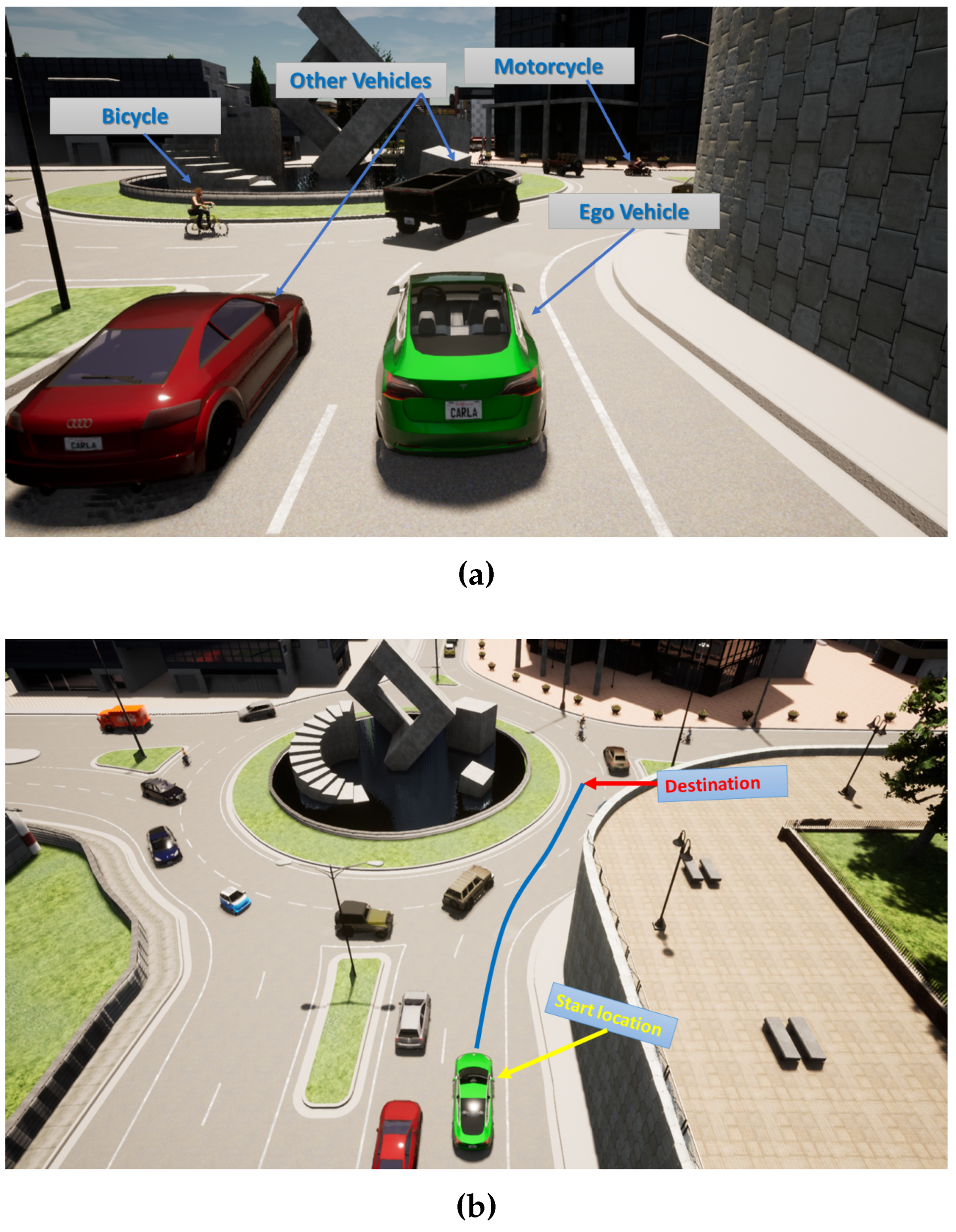
  • We address the problem of entering roundabouts with dense traffic involving other vehicles, cyclists, and motorcycles.
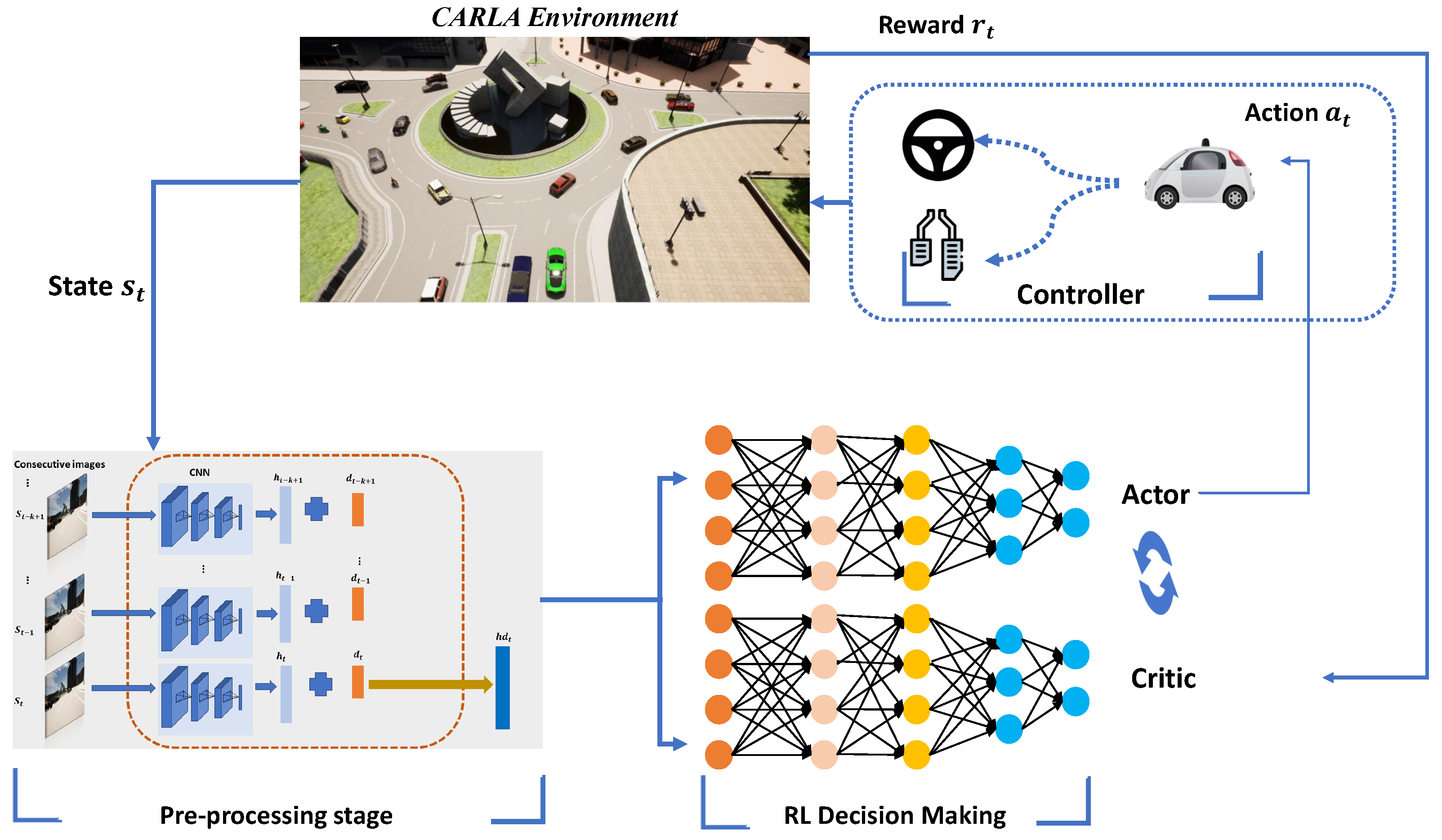
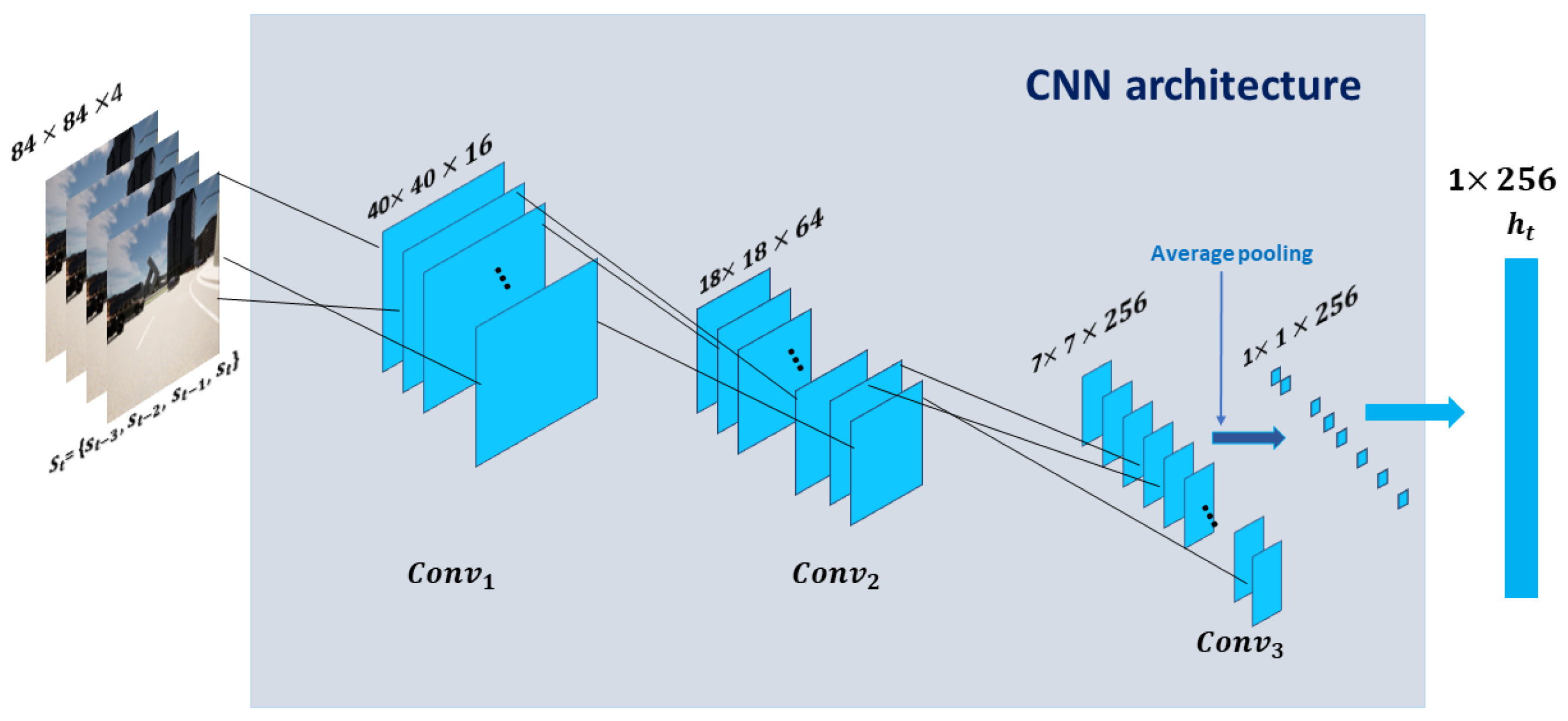
  • We propose a modified SAC algorithm in combination with CNN to extract the main features of images captured by the front camera of the AV. We combine those features with the description vector to help the AV reach its destination quickly.
  • We compare our model with DQN and PPO algorithms. The results demonstrate that SAC outperforms traditional DQN and PPO models.
The remainder of the paper is organized as follows. Section 2 discusses the related work on applying DRL algorithms for autonomous navigation and decision-making in the context of AVs while shedding light on the novelty of our proposed approach compared to existing ones. Section 3 presents an overview of reinforcement learning. Section 4 introduces our approach by presenting the Soft Actor-Critic (SAC) model, the state space, the action space, and the reward function. Section 5 presents the simulator used to train and validate our model, discusses our results obtained by SAC, and compares them with the DQN and PPO models. The last Section 6, concludes our paper and discusses future perspectives.

2. Related Work

The reason behind the widespread interest in DRL algorithms is their exceptional data handling capacity and ability to capture intricate states in high-dimensional spaces, specifically in the robotics field [20]. Their application in Unmanned Ground Vehicles (UGV) [21] is particularly noteworthy; DRL algorithms are increasingly being investigated for autonomous navigation tasks.
An example of such behavior in this domain is the number of works showing new ways of extracting decision-making and control commands from laser scans [22,23]. What distinguishes them from other methods used is that they can smoothly switch between simulated models and actual situations that demonstrate good performance over time in terms of transferability. This further underscores the robustness and effectiveness of these algorithms in practical applications.
According to [24], the study addresses the issue of mixed traffic involving human-driven vehicles (HVs) and AVs. It advocates for an approach based on deep Q-networking for managing AV movement through intersections aimed at enhancing the efficiency of road utilization as well as safety levels. It shows its superiority over existing methods, especially in dynamic traffic environments, effectively reducing driving distance, time, and waiting time for AVs.
Elallid et al. [25] presents an approach that uses DRL to control AV driving through intersections with high traffic. Their DRL framework is implemented based on DQN to achieve an effective navigation strategy in the presence of other road users. The results show that their model reduces travel time delays while avoiding collisions when compared with existing traffic control methods.
Wang et al. [26] introduced a reinforcement-learning (RL) method for self-driving cars in complex traffic conditions. The paper aimed to speed up learning by using motion skills and the prior knowledge of experts. It used expert demonstrations and a double initialization strategy in order to optimize leveraging expert priors. According to their experiments, it is shown that this model outperforms other models with regard to learning efficiency and driving performance in heavy traffic.
Chen et al. [27] address the challenge of on-ramp merging for AVs in mixed traffic. They formulate the problem as a MARL task and develop an efficient MARL algorithm with features such as action masking, local rewards, curriculum learning, and parameter sharing. The proposed approach consistently outperforms state-of-the-art benchmarks in terms of training efficiency and collision rate.
Wang et al. [28] present a DRL-based lane-changing model for autonomous vehicles in mixed traffic. The model uses an analysis of natural driving trajectories to build a lane-changing environment at the vehicle group level. In order to mimic mixed flow situations, it uses the SAC algorithm to adjust velocity while taking into account the trajectories of surrounding vehicles. Training and testing on real-world data show that the model achieves a 90% success rate in lane-changing without a collision. In terms of safety and efficiency evaluation indicators, the system improves both safety and efficiency when compared to human driving.
Zengrong et al. [29] tackle the challenge of ensuring both safety and efficiency for AVs navigating unsignaled roundabouts. They propose a driving policy based on the SAC algorithm, enhanced with interval prediction and self-attention mechanisms, to focus on potential conflict vehicles and predict driving risks. The algorithm was trained in a low-dimensional environment and validated in the CARLA simulator. Results show a 15% reduction in collisions, improved safety, and effective decision-making at roundabout entrances and exits. However, their work is tested only in CARLA without training to catch more skills and did not include the perception model or take into account high mobility.
The paper by [30] explores optimizing traffic dynamics with a mix of AVs and human-driven vehicles (HVs) using the PPO algorithm. In a roundabout scenario, the study found that a higher presence of AVs of 80% reduces travel time and pollution and is perceived as safer and smoother by human participants compared to a lower presence of 20%. The results indicate that AVs can significantly improve urban traffic efficiency and safety. However, this work did not include a perception model and did not take into consideration dense traffic, which is the most complex scenario
Jingpeng et al. [31] address the challenge of improving the efficiency and safety of AVs in navigating unsignaled roundabout scenarios with low penetration. They propose an optimization-based behavioral choice model using the PPO algorithm. They used the CoordConv network for spatial perception to capture and store low-dimensional environmental information. The results demonstrate that their model achieves an improvement in reward value function, training efficiency, and traversal time in simulations with varying numbers of vehicles, outperforming the PPO+CCMR algorithm, especially when fewer vehicles are present.
The paper [32] addresses the problem of predicting potential conflict risks in roundabout merging scenarios to enhance active safety. It develops a hybrid deep learning framework using a CNN and a long short-term memory network (LSTM), integrated with the convolutional block attention module (CBAM). The framework utilizes an improved 2D-TTC indicator and analyzes vehicle characteristics through a roundabout coordinate system. The findings show that the proposed model outperforms benchmark models, with segmental predictions being more accurate than overall predictions. Additionally, specific vehicle groups significantly impact conflict risk prediction, and understanding these dynamics can improve safety management at roundabouts.
In light of the existing literature, it is important to acknowledge that previous studies have mostly focused on controlling AVs in simplified environments, frequently ignoring the complex dynamics involving various road participants, such as other vehicles, cyclists, and motorcyclists. Furthermore, some approaches have not been trained and tested in dense traffic scenarios.
In light of these limitations, we are motivated to provide a novel solution that can address high-mobility scenarios, especially those that arise in roundabouts with heavy traffic. To improve the realism of our model, we chose to use the three-dimensional CARLA simulator for both the training and validation stages.

3. Deep Reinforcement Learning: An Overview

In recent years, DRL has made significant progress, becoming widely embraced across various fields, particularly robotics. Previous studies have highlighted the effectiveness of the model-free DRL approach in enabling autonomous acquisition of motion control strategies. This recognition has led to substantial efforts to advance methodologies based on DRL. At its core, a reinforcement learning algorithm operates based on the principles of a Markov decision process (MDP), where the system’s current state depends solely on the preceding state, regardless of the specific path taken. MDPs are typically represented as a tuple ( S , A , R , P ) , where S denotes the state space of the environment, A represents the available actions, R indicates the rewards or feedback received from taking actions at each time step, and P characterizes the probability distribution governing state transitions [33].
At each time step, the RL agent observes the state s t from the set S and takes action a t from the set A , subsequently receiving an immediate reward r t = R ( s t , a t ) where R is a function mapping states and actions to real numbers: S × A R . Additionally, the agent transitions to the next state s t + 1 S based on the transition probability P ( s t + 1 | s t , a t ) , which is a function mapping state-action pairs to probabilities in the range [ 0 , 1 ] : S × A [ 0 , 1 ] .
In RL, the agent typically determines its action through a policy denoted as a t π ( · | s t ) wherein π is considered a probability distribution reflecting the agent’s beliefs regarding its decisions at each time step within its environment. The objective for the RL agent is to maximize the cumulative reward or total return as it progresses from an initial state s. This cumulative reward, denoted as V π ( s ) , is expressed as the expected value under the distribution P , calculated across successive time steps from t = 0 to T, wherein each reward r t is discounted by a factor γ t . The expression for V π ( s ) is as follows:
V π ( s ) = E s t P t = 0 T γ t · r t
The function denoted as V π is recognized as the value function, while γ is the discounting factor, which must adhere to the constraint of 0 < γ 1 . In a similar vein, the state-value function, Q π , is contingent upon the state s t and the action a t at time step t, as follows:
Q π ( s t , a t ) = r t + γ · E s t + 1 P [ V π ( s t + 1 ) ] = r t + γ · E s t + 1 P , a t + 1 π [ Q π ( s t + 1 , a t + 1 ) ]
DRL algorithms are generally categorized into two main types: discrete algorithms, such as Deep Q-Network (DQN) and its variant Double Deep Q-Network (DDQN) and continuous algorithms, which include diverse methods like stochastic policy techniques (e.g., Asynchronous Advantage Actor-Critic (A3C)) and deterministic techniques (e.g., Deep Deterministic Policy Gradient (DDPG)). In the actor-critic framework, a fundamental RL paradigm, two distinct neural networks are employed: the actor-network takes the state as input and predicts optimal actions, while the critic network evaluates the quality of the actor’s actions.

4. Methodology

The objective of this study is to ensure the safe navigation of AVs as they approach roundabouts, reducing the risk of collisions with other vehicles by using the SAC algorithm. Our proposed framework is represented in Figure 1.
We start by introducing the SAC algorithm, followed by describing the state space, the action space, and the reward function of our model.

4.1. Soft Actor-Critic

Soft Actor-Critic (SAC) represents a progressed approach within advanced deep reinforcement learning, characterized by its policy-based and model-free nature. Compared to traditional RL methods, SAC uses the concept of soft strategy optimization. Rather than focusing on maximizing rewards, SAC integrates the notion of entropy into its optimization strategy to strike a balance between exploration and exploitation. This approach allows the agent to handle tasks with a degree of randomness by enhancing adaptability and flexibility. Consequently, SAC excels at tackling continuous action spaces, leading to notable enhancements in learning efficiency and stability [34].
Integrating maximum policy entropy into the SAC algorithm aims to encourage the agent’s exploration of its environment. This allows the agent to achieve optimal actions, improving the model’s capacity for generalization.
The primary objective of the RL algorithm is to learn a policy that maximizes the expected future accumulated return π * = arg max π V π ( s ) and V π , which is computed by the Equation (1). In addition to the fundamental objectives outlined earlier, the maximum entropy reinforcement learning approach necessitates maximizing the action entropy for every policy output as follows:
π * = arg max π t = 0 T γ t · r t + α H ( π ( · | s t ) )
The definition of every policy entropy H is as follows:
H ( π ( · | s ) ) = a A π ( a | s ) log ( π ( a | s ) ) d a = E a π ( · | s ) log ( π ( a | s ) )
This goal is to enhance how effectively the policy explores by boosting both the anticipated future rewards and policy unpredictability. The temperature parameter, represented by α , determines the significance of the unpredictability compared to the rewards. Maximum entropy RL methodically converges toward conventional RL as α 0 . According to the Bellman Equation (2), we can obtain the updated soft Bellman equation:
Q π ( s t , a t ) = r t + γ · E s t + 1 P , a t + 1 π [ Q π ( s t + 1 , a t + 1 ) α log ( π ( a t + 1 | s t + 1 ) ) ]
One common technique that is extensively utilized in the SAC algorithm is double Q-networks to address the overestimation issue. Hence, the parameters of the critic network of SAC are updated by minimizing the mean Bellman-squared error (MBSE) loss function:
L critic ( θ i ) = E s t P , a t π Q θ i π ( s t , a t ) r t + γ · Q ^ π 2
Where Q ^ π is the state-action value of the next step from double target Q-networks and computed as follows:
Q ^ π = E s t + 1 P , a t + 1 π min i = 1 , 2 Q target , i ( s t + 1 , a t + 1 ) α log π ( a t + 1 | s t + 1 )
Combining these equations, the total critic loss is the sum of the individual losses for each Q-network:
L critic ( θ ) = L critic , 1 ( θ 1 ) + L critic , 2 ( θ 2 )
The loss function for the actor in the SAC model is designed to maximize the expected return while integrating an entropy term to encourage exploration. The actor aims to learn a policy π ϕ that outputs actions that maximize the expected Q-value as estimated by the critics, adjusted by the entropy of the policy. The actor loss L actor is given by:
L actor ( ϕ ) = E s t P , a t π ϕ ( · s t ) α log π ϕ ( s t a t ) min i = 1 , 2 Q π ( s t , a t )

4.2. State Space

In our scenario, we process a stack of four RGB images captured by the front camera of the AV. Initially, these images have dimensions of 800 × 600 × 3 × 4 pixels. We resize and reduce them to 84 × 84 × 3 × 4 pixels, and then convert them to grayscale. This transformation yields a new state, denoted as s t , with dimensions of 84 × 84 × 4 , which are fed into the input of the neural network. The architecture comprises three convolutional (Conv) layers, all featuring kernel sizes of 5 × 5 . Each layer contains 16, 16, and 64 kernels, respectively. Strided convolutions with a stride value of 2 are applied across all three layers. Additionally, we employ average pooling with an output size of 1.
In the diagram provided (see Figure 2), the architecture comprises three Convolutional (Conv) layers followed by average pooling. The feature maps resulting from these layers have dimensions of 40 × 40 × 16 , 18 × 18 × 64 , 7 × 7 × 256 , and 1 × 1 × 256 , successively. Finally, these features are flattened into a vector denoted as h t , with a dimensionality of 1 × 1 × 256 . We can use the function f C N N s , depicted as follows:
f C N N s ( s t ) = h t
where s t R 84 × 84 × 4 and h t R 256 .
To ensure the AV reaches its intended destination effectively, it is crucial to integrate the current state h t with the destination vector dest t R 2 . This destination vector is expressed as dest t = [ X d e s t X A V , Y d e s t Y A V ] , where X d e s t and Y d e s t denote the x and y coordinates of the destination position, while X A V and Y A V represent the corresponding coordinates of the AV at each time step t as shown in Figure 3. Subsequently, the update function is as follows:
f C N N s ( s t , dest t ) = h d t , h d t R 258

4.3. Action Space

In the Carla simulator environment, the AV interacts with its environment using three main control commands: acceleration, steering, and braking. These commands are represented as float values with ranges: [ 0 , 1 ] for acceleration, [ 1 , 1 ] for steering, and [ 0 , 1 ] for braking. The SAC algorithm is known as a continuous DRL algorithm, and it necessitates selecting actions in a continuous manner. Hence, at each time step t, the agent’s action a t comprises a tuple ( acceleration t , steering t , brake t ) , with each one within its respective command range.
DQN is a discrete DRL algorithm, the agent must make discrete action choices as per Table 1.

4.4. Reward Function

Inspired by [35], we have designed our reward system to align with the challenges posed by urban traffic conditions. Our aim is to guide AVs safely through roundabouts without collisions while ensuring their timely arrival at their destinations. To achieve this objective, our reward system is structured as four pivotal components: maintaining the speed of the AV, penalizing collisions, ensuring the AV respects its lane by avoiding unauthorized lane changes and considering the remaining distance to the destination.
For simplification, we define the current distance to the destination as d cu and the previous distance as d pre . The AV’s forward speed is denoted by v speed , while the measure of the AV if moving off-road and in another lane is represented by M offroad and M otherlane . In the case of collisions, a penalty denoted as C collision = 100 is enforced, adjusting the reward ( R t 1 ) accordingly.
Furthermore, if the AV approaches the goal ( d p r e > d c u ), it receives an augmented reward ( R t 2 ) in order to encourage the AV to progress towards the destination. Moreover, the AV’s velocity should not surpass the speed limit value of 3 (derived from 30 divided by 10), designated as R t 3 .
Maintaining the AV to respect its lane is important; we penalize the agent with minor penalties if the AV is traveling in an unauthorized lane or off-road, as represented in R t 4 and R t 5 . Ultimately, if the AV arrives at the intended destination successfully, it is rewarded by R t 6 = 100 . The reward function can be represented as follows:
r e w a r d = R t 1 = C collison R t 2 = d pre d cu R t 3 = v speed 10 v speed [ 0 , v limit ] R t 4 = 0.05 × M offroad R t 5 = 0.05 × M otherlane R t 6 = 100 R t = R t 1 + R t 2 + R t 4 + R t 5 + R t 6

4.5. Training Models

DQN model: Our model training methodology aims to effectively train a neural network for decision-making in dynamic environments. Initially, the neural network is initialized with random weights. The agent starts taking random actions to explore the environment, and during episodes, it exploits the knowledge learned during exploration. Actions taken by the agent are stored in a replay buffer with their corresponding states. s t , destination vector d t , rewards r t , next destination vector d t + 1 , and next states s t + 1 , forming tuples of the form ( s t , d t , a t , r t , s t + 1 , d t + 1 ) .
During the training phase, the model selects a random batch, typically consisting of 128 samples, from the replay buffer. This batch is then fed through the policy network, which predicts Q-values associated with each action. Subsequently, to update the Q-value according to Equation (2), a second pass through the network is necessary to compute the maximum Q-value for the next action, a t + 1 . This additional pass is facilitated by what is known as the target network.
Following this, the loss between the predicted Q-value and the output from the target network is computed using the mean square error (MSE) metric. The ADAM optimizer [36] is then utilized to minimize this loss, enabling the updating of weights through backpropagation. This iterative process allows the neural network to progressively refine its Q-value predictions, thereby improving the agent’s decision-making capabilities throughout the training process. By iteratively adjusting the network’s weights based on experiences gathered from the replay buffer, the model adapts and learns to make more informed decisions in dynamic environments.
PPO model: The training process for the PPO algorithm follows several key steps. Initially, two neural networks are initialized: an actor and a critic. The actor-network uses a tanh activation function in the output layer to generate the probability distribution over actions, while the critic network, which estimates the state value, employs a tanh activation function in its output layer.
The agent interacts with the environment, then the samples are collected according to the current policy. The advantages are computed and returned for each time step in the collected trajectories. The PPO objective is defined as follows:
L ( θ ) = E t min π θ ( a t | s t ) π θ old ( a t | s t ) A t , clip π θ ( a t | s t ) π θ old ( a t | s t ) , 1 ϵ , 1 + ϵ A t
where A t the advantage function from the finite-horizon estimation of T steps is given as:
A t = μ t + ( γ λ ) μ t + 1 + ( γ λ ) 2 μ t + 2 + . . . + ( γ λ ) T t + 1 μ T 1
and μ t = r t + γ V ( s t + 1 ) V ( s t )
The objective function L ( θ ) is then used to update the parameters of both the actor and critic networks. This objective ensures stable policy updates by preventing large changes in the policy. By iterating through these steps, the policy and value function are gradually refined in order to enhance the agent’s performance in the environment.
SAC model: The agent interacts with the environment according to its probabilistic policy, denoted as π θ ( · | s t ) . This policy allows a balance between exploitation and exploration. In our implementation, we use Gaussian policy, wherein the policy network generates two parameters that define the mean and standard deviation of a Gaussian distribution, thus yielding actions represented as a t N ( μ θ ( s t ) , σ θ ( s t ) ) .
To preserve the differentiability of the stochastic policy, we employ the reparameterization trick. This technique involves deriving action samples from the stochastic policy by evaluating a deterministic function as follows:
a t = tanh ( μ θ ( s t ) + σ θ ( s t ) ξ ) , ξ N ( 0 , I )
Here, ξ indicates independent Gaussian noise, while the application of hyperbolic tangent ensures that actions are bounded within a finite range.
Our framework utilizes two Q-networks, the critic and target critic networks. Those networks are necessary to ensure the stability of the learning process. The network’s weights are updated through the Q-network to ensure the agent’s adaptation to the environment over time. Similar to the DQN approach, the tuple ( s t , d t , a t , r t , s t + 1 , d t + 1 ) is stored in a replay buffer. During training, the model randomly selects batches of data from this replay buffer. This allows the agent to learn from past experiences, breaking correlations in the data and promoting more robust and efficient learning. To better illustrate the implementation of our approach, we provide Algorithm 1.
The other settings of our models are represented in Table 2:
Algorithm 1 Soft Actor-Critic with Destination Vector
1:
Initialize actor network parameters ϕ and critic network parameters θ .
2:
Initialize the entropy coefficient α .
3:
Define the batch size N and create an empty replay buffer D .
4:
Set target network parameters equal to the critic parameters: θ target θ .
5:
for each episode e = 1 to E do
6:
    Initialize images state s t C a r l a E n v .
7:
    Initialize destination vector dest t C a r l a E n v .
8:
    for each step t from 1 to N steps  do
9:
          Select an action a t π ϕ ( a t | ( s t , dest t ) )
10:
        Interact with the environment:
11:
        Observe the next state s t + 1 , reward r t , and next destination dest t + 1
12:
        Store the transition in the replay buffer:
13:
         D D ( s t , dest t , a t , r t , s t + 1 , dest t + 1 )
14:
        if time to update the critic network then
15:
           Sample a batch of transitions ( s t i , dest t i , a t i , r t i , s t + 1 i , dest t + 1 i ) i = 1 N from D
16:
           Compute the loss for the critic L critic ( θ ) using Equations (6) and (8)
17:
           Update the critic network parameters θ
18:
        end if
19:
        if time to update the actor network then
20:
           Sample a batch of transitions ( s t i , dest t i , a t i , r t i , s t + 1 i , dest t + 1 i ) i = 1 N from D
21:
           Compute the loss for the actor L actor ( ϕ ) using Equation (9)
22:
           Update the actor network parameters ϕ
23:
           if automatic entropy tuning is enabled then
24:
               Adjust the entropy coefficient α
25:
           end if
26:
        end if
27:
        if time to update the target network then
28:
           Update the target network parameters: θ target θ
29:
        end if
30:
    end for
31:
end for

5. Experiments

In this section, we present our simulation setup, highlighting our simulator used for both training and validation purposes. Additionally, we provide a comprehensive analysis of results obtained in the training and testing phases.

5.1. Training Setting

We conducted extensive experiments in the CARLA simulator (version 0.9.10) with PyTorch for controlling autonomous driving within a challenging roundabout scenario. CARLA offers hyper-realistic physics to train and validate models in an environment close to the real world [37].
Within this scenario, vehicles encountered numerous complexities, including maneuvering through multiple lanes, navigating through oncoming traffic, merging seamlessly with existing flows, and prioritizing pedestrian safety at designated crosswalks. The complexity of these challenges stems from the real-time decisions and good responses required for safe and efficient navigation.
To ensure realism in our approach, we spawn diverse road participants in the traffic, including pedestrians, cars, bicycles, and motorcycles. This allows us to test and assess the performance of our autonomous driving algorithm across a wide range of traffic scenarios and obstacles.
To recreate challenging traffic scenarios, we adjusted various factors like how fast vehicles move, the distance between them, and how often new vehicles enter the simulation. This helps us simulate situations on the road that closely resemble real-world driving scenarios. Then, we test our model in complex driving situations to achieve a robust evaluation.
Furthermore, we integrated CARLA with Gym, an open-source Python library developed by OpenAI [38]. It was designed for reinforcement learning algorithm development and evaluation, and Gym served as an interface to facilitate communication between the DRL algorithm and the simulation environment.
Figure 4 represents a roundabout where the AV must navigate smoothly while ensuring the safety of all road users, including cyclists, motorcycles, and other vehicles. This scenario involves the presence of 120 vehicles moving in randomly, including motorcycles, cyclists, and four-wheeled vehicles, all controlled by the CARLA traffic manager.
All vehicles except our AV are in autopilot mode. Each vehicle maintains a safe distance of 2.5 m from others and respects a speed limit of 30 ms. The objective is to facilitate the AV’s entry into the roundabout without any collisions, thereby ensuring smooth and safe traffic flow.
The simulator begins by capturing images at an initial size of 800 × 600 pixels. To minimize data overload, we choose to capture 5 frames per second (fps) during both the training and testing phases. Training episodes end based on the following conditions: (1) If a collision occurs between the AV and other road users; (2) If the AV successfully arrives at its destination; (3) If the number of episodes exceeds the maximum number of training steps, which is set at 1100.

5.2. Training and Testing Results

In this section, we present the performance of our model SAC compared to the DQN model.
To show the learning performance in DRL, we often reward it as a standard criterion. Figure 5 shows the average reward of SAC, PPO, and DQN algorithms during training. We note that SAC converges faster than the PPO and DQN modes and achieves a high score of approximately 91.9. However, PPO achieves around 58.4, and its curve is not very similar to the curve of SAC. Furthermore, we notice that DQN is very low in terms of convergence and achieves only a 36.6 score, which shows the superiority of our model SAC compared to the two preceding models.
We employ the average success rate as the main assessment metric in order to fairly assess the performance of the suggested framework in various scenarios, and each scenario depends on the number of AVs spawned in our environment. We have selected four specific densities for evaluation as follows: AVs = 120 , AVs = 140 , AVs = 160 , and AVs = 210 .
Throughout the testing phase, we employ extra metrics, such as the collision rate, average time, average speed, average traveled distance, average steps, and average reward.
  • Success rate (Succ %): During testing, we test our model for 50 episodes, and we compute the percentage of episodes in which the AV successfully reaches its destination.
  • Collision rate ( Coll %): It computes the percentage of episodes when the AV collides with other vehicles. It is considered critical safety performance.
  • Average time (Avg. time): It counts the time it takes for the AV to reach its destination in each episode. We computed the average time of 50 episodes.
  • Average speed (Avg. Speed): It computes the average speed of the AV during episodes.
  • Average Traveled Distance (Avg. Dis): is the distance traveled by the AV from its start location to its destination.
  • Average Steps (Avg. Steps): the number of steps that it takes for the AV to attain its destination.
Table 3 illustrates the quantitative comparison between the SAC, PPO, and DQN models according to the previous metrics. We remark that the SAC model achieved the best results compared to the PPO and DQN models in all metrics. Despite the high density of AVs in the fourth scenario, we notice that SAC attains a 94% success rate, demonstrating the effectiveness of SAC compared to PPO and DQN, which reach 80% and 52% success rates, respectively. Moreover, SAC shows superior performance in controlling AVs to reach their destinations quickly, as shown by the average number of steps and average time spent in the four densities.
Furthermore, the collision rate is very low, at 2% in the first three densities and 6% in the last density, indicating that SAC successfully avoids collisions with other vehicles, ensuring safety on the road. In contrast, PPO and DQN have a high number of crashes with vehicles, especially in the last density where the number of AVs is very high.
Additionally, our model shows that the AV’s traveled distance from its start location to its destination is around 32 m in all directions, which demonstrates that our approach is successful in finding the optimal path to the destination. However, PPO and DQN achieve around 33 m and 34 m in the traveled distance, respectively.

6. Conclusions

This paper introduces DRL to enhance the vehicle control capabilities of AVs. Our focus is on addressing the slow convergence of traditional RL models in complex scenarios with dense traffic, particularly roundabout scenarios.
To overcome this challenge, we propose a Soft Actor-Critic to guide an AV to reach its destination quickly without colliding with other vehicles. To achieve this, we utilize a CNN model to extract the main features from four consecutive images captured by the front camera of the AV. Then, we concatenate these features with the destination vector and feed them to the SAC model to make decisions. We test and validate our model in the CARLA simulator, which is the most powerful simulator for autonomous driving applications. The results demonstrate the superiority of our model compared to the DQN and PPO models in terms of convergence, high success rate, and low collision rate.
In future work, we aim to tackle even more complex scenarios and improve the SAC algorithm by integrating CNN and attention mechanisms to benefit from previous information as AVs navigate within their environment.

Author Contributions

Conceptualization and methodology, B.B.E., N.B, M.B. and Y.H.-A.; investigation, N.B. and Y.H.-A.; writing—original draft preparation, B.B.E.; supervision, N.B., M.B. and Y.H.-A. All authors have read and agreed to the published version of the manuscript.

Funding

This research received no external funding.

Data Availability Statement

The data presented in this study are available in a controlled manner on request from the corresponding author due to the interests of confidentiality.

Conflicts of Interest

The authors declare no conflict of interest.

Abbreviations

The following abbreviations are used in this manuscript:
DRLDeep Reinforcement Learning
SACSoft Actor-Critic
DQNDeep Q-Network
DDPGDeep Deterministic Policy Gradient
DLDeep Learning
AIArtificial Intelligence
MDPMarkov Decision Process
CNNConvolutional Neural Networks
AVsAutonomous Vehicles

References

  1. Qureshi, K.N.; Abdullah, A.H. A survey on intelligent transportation systems. Middle-East J. Sci. Res. 2013, 15, 629–642. [Google Scholar]
  2. Fadhel, M.A.; Duhaim, A.M.; Saihood, A.; Sewify, A.; Al-Hamadani, M.N.; Albahri, A.; Alzubaidi, L.; Gupta, A.; Mirjalili, S.; Gu, Y. Comprehensive Systematic Review of Information Fusion Methods in Smart Cities and Urban Environments. Inf. Fusion 2024, 107, 102317. [Google Scholar] [CrossRef]
  3. Be. Road Traffic Injuries. 2021. Available online: https://www.who.int/news-room/fact-sheets/detail/road-traffic-injuries (accessed on 2 April 2024).
  4. Gulzar, M.; Muhammad, Y.; Muhammad, N. A survey on motion prediction of pedestrians and vehicles for autonomous driving. IEEE Access 2021, 9, 137957–137969. [Google Scholar] [CrossRef]
  5. Elallid, B.B.; El Alaoui, H.; Benamar, N. Deep Reinforcement Learning for Autonomous Vehicle Intersection Navigation. In Proceedings of the 2023 International Conference on Innovation and Intelligence for Informatics, Computing, and Technologies (3ICT), Sakheer, Bahrain, 20–21 November 2023; pp. 308–313. [Google Scholar]
  6. Sadaf, M.; Iqbal, Z.; Javed, A.R.; Saba, I.; Krichen, M.; Majeed, S.; Raza, A. Connected and automated vehicles: Infrastructure, applications, security, critical challenges, and future aspects. Technologies 2023, 11, 117. [Google Scholar] [CrossRef]
  7. Yu, G.; Li, H.; Wang, Y.; Chen, P.; Zhou, B. A review on cooperative perception and control supported infrastructure-vehicle system. Green Energy Intell. Transp. 2022, 1, 100023. [Google Scholar] [CrossRef]
  8. Bachute, M.R.; Subhedar, J.M. Autonomous driving architectures: Insights of machine learning and deep learning algorithms. Mach. Learn. Appl. 2021, 6, 100164. [Google Scholar] [CrossRef]
  9. Wang, L.; Zhang, X.; Song, Z.; Bi, J.; Zhang, G.; Wei, H.; Tang, L.; Yang, L.; Li, J.; Jia, C.; et al. Multi-modal 3d object detection in autonomous driving: A survey and taxonomy. IEEE Trans. Intell. Veh. 2023, 8, 3781–3798. [Google Scholar] [CrossRef]
  10. Aradi, S. Survey of deep reinforcement learning for motion planning of autonomous vehicles. IEEE Trans. Intell. Transp. Syst. 2020, 23, 740–759. [Google Scholar] [CrossRef]
  11. Garrido, F.; Resende, P. Review of decision-making and planning approaches in automated driving. IEEE Access 2022, 10, 100348–100366. [Google Scholar] [CrossRef]
  12. Kuutti, S.; Bowden, R.; Jin, Y.; Barber, P.; Fallah, S. A survey of deep learning applications to autonomous vehicle control. IEEE Trans. Intell. Transp. Syst. 2020, 22, 712–733. [Google Scholar] [CrossRef]
  13. Elallid, B.B.; Benamar, N.; Hafid, A.S.; Rachidi, T.; Mrani, N. A Comprehensive Survey on the Application of Deep and Reinforcement Learning Approaches in Autonomous Driving. J. King Saud-Univ.-Comput. Inf. Sci. 2022, 34, 7366–7390. [Google Scholar] [CrossRef]
  14. Berge, S.H.; de Winter, J.; Cleij, D.; Hagenzieker, M. Triangulating the future: Developing scenarios of cyclist-automated vehicle interactions from literature, expert perspectives, and survey data. Transp. Res. Interdiscip. Perspect. 2024, 23, 100986. [Google Scholar] [CrossRef]
  15. Chao, Q.; Bi, H.; Li, W.; Mao, T.; Wang, Z.; Lin, M.C.; Deng, Z. A survey on visual traffic simulation: Models, evaluations, and applications in autonomous driving. In Computer Graphics Forum; Wiley Online Library: Hoboken, NJ, USA, 2020; Volume 39, pp. 287–308. [Google Scholar]
  16. Yadav, P.; Mishra, A.; Kim, S. A comprehensive survey on multi-agent reinforcement learning for connected and automated vehicles. Sensors 2023, 23, 4710. [Google Scholar] [CrossRef]
  17. Elallid, B.B.; Abouaomar, A.; Benamar, N.; Kobbane, A. Vehicles control: Collision avoidance using federated deep reinforcement learning. In Proceedings of the GLOBECOM 2023-2023 IEEE Global Communications Conference, Kuala Lumpur, Malaysia, 4–8 December 2023; pp. 4369–4374. [Google Scholar]
  18. Han, Y.; Wang, M.; Leclercq, L. Leveraging reinforcement learning for dynamic traffic control: A survey and challenges for field implementation. Commun. Transp. Res. 2023, 3, 100104. [Google Scholar] [CrossRef]
  19. Teng, S.; Hu, X.; Deng, P.; Li, B.; Li, Y.; Ai, Y.; Yang, D.; Li, L.; Xuanyuan, Z.; Zhu, F.; et al. Motion planning for autonomous driving: The state of the art and future perspectives. IEEE Trans. Intell. Veh. 2023, 8, 3692–3711. [Google Scholar] [CrossRef]
  20. Huang, W.; Braghin, F.; Wang, Z. Learning to drive via apprenticeship learning and deep reinforcement learning. In Proceedings of the 2019 IEEE 31st International Conference on Tools with Artificial Intelligence (Ictai), Portland, OR, USA, 4–6 November 2019; pp. 1536–1540. [Google Scholar]
  21. Pfeiffer, M.; Shukla, S.; Turchetta, M.; Cadena, C.; Krause, A.; Siegwart, R.; Nieto, J. Reinforced imitation: Sample efficient deep reinforcement learning for mapless navigation by leveraging prior demonstrations. IEEE Robot. Autom. Lett. 2018, 3, 4423–4430. [Google Scholar] [CrossRef]
  22. Cimurs, R.; Suh, I.H.; Lee, J.H. Goal-driven autonomous exploration through deep reinforcement learning. IEEE Robot. Autom. Lett. 2021, 7, 730–737. [Google Scholar] [CrossRef]
  23. Reda, M.; Onsy, A.; Haikal, A.Y.; Ghanbari, A. Path planning algorithms in the autonomous driving system: A comprehensive review. Robot. Auton. Syst. 2024, 174, 104630. [Google Scholar] [CrossRef]
  24. Moon, S.; Koo, S.; Lim, Y.; Joo, H. Routing Control Optimization for Autonomous Vehicles in Mixed Traffic Flow Based on Deep Reinforcement Learning. Appl. Sci. 2024, 14, 2214. [Google Scholar] [CrossRef]
  25. Elallid, B.B.; Bagaa, M.; Benamar, N.; Mrani, N. A reinforcement learning based approach for controlling autonomous vehicles in complex scenarios. In Proceedings of the 2023 International Wireless Communications and Mobile Computing (IWCMC), Marrakesh, Morocco, 19–23 June 2023; pp. 1358–1364. [Google Scholar]
  26. Wang, L.; Liu, J.; Shao, H.; Wang, W.; Chen, R.; Liu, Y.; Waslander, S.L. Efficient Reinforcement Learning for Autonomous Driving with Parameterized Skills and Priors. arXiv 2023, arXiv:2305.04412. [Google Scholar]
  27. Chen, D.; Hajidavalloo, M.R.; Li, Z.; Chen, K.; Wang, Y.; Jiang, L.; Wang, Y. Deep multi-agent reinforcement learning for highway on-ramp merging in mixed traffic. IEEE Trans. Intell. Transp. Syst. 2023, 24, 11623–11638. [Google Scholar] [CrossRef]
  28. Wang, Z.; Huang, H.; Tang, J.; Hu, L. A deep reinforcement learning-based approach for autonomous lane-changing velocity control in mixed flow of vehicle group level. Expert Syst. Appl. 2024, 238, 122158. [Google Scholar] [CrossRef]
  29. Wang, Z.; Liu, X.; Wu, Z. Design of Unsignalized Roundabouts Driving Policy of Autonomous Vehicles Using Deep Reinforcement Learning. World Electr. Veh. J. 2023, 14, 52. [Google Scholar] [CrossRef]
  30. Ferrarotti, L.; Luca, M.; Santin, G.; Previati, G.; Mastinu, G.; Gobbi, M.; Campi, E.; Uccello, L.; Albanese, A.; Zalaya, P.; et al. Autonomous and Human-Driven Vehicles Interacting in a Roundabout: A Quantitative and Qualitative Evaluation. IEEE Access 2024, 12, 32693–32705. [Google Scholar] [CrossRef]
  31. Gan, J.; Zhang, J.; Liu, Y. Research on behavioral decision at an unsignalized roundabout for automatic driving based on proximal policy optimization algorithm. Appl. Sci. 2024, 14, 2889. [Google Scholar] [CrossRef]
  32. Li, Y.; Ge, C.; Xing, L.; Yuan, C.; Liu, F.; Jin, J. A hybrid deep learning framework for conflict prediction of diverse merge scenarios at roundabouts. Eng. Appl. Artif. Intell. 2024, 130, 107705. [Google Scholar] [CrossRef]
  33. Qi, J.; Zhou, Q.; Lei, L.; Zheng, K. Federated reinforcement learning: Techniques, applications, and open challenges. arXiv 2021, arXiv:2108.11887. [Google Scholar] [CrossRef]
  34. Haarnoja, T.; Tang, H.; Abbeel, P.; Levine, S. Reinforcement learning with deep energy-based policies. In Proceedings of the International Conference on Machine Learning, Sydney, Australia, 6–11 August 2017; pp. 1352–1361. [Google Scholar]
  35. Palanisamy, P. Hands-On Intelligent Agents with OpenAI Gym: Your Guide to Developing AI Agents Using Deep Reinforcement Learning; Packt Publishing: Birmingham, UK, 2018. [Google Scholar]
  36. Kingma, D.P.; Ba, J. Adam: A method for stochastic optimization. arXiv 2014, arXiv:1412.6980. [Google Scholar]
  37. Dosovitskiy, A.; Ros, G.; Codevilla, F.; Lopez, A.; Koltun, V. CARLA: An Open Urban Driving Simulator. In Proceedings of the 1st Annual Conference on Robot Learning, Mountain View, CA, USA, 13–15 November 2017; pp. 1–16. [Google Scholar]
  38. Brockman, G.; Cheung, V.; Pettersson, L.; Schneider, J.; Schulman, J.; Tang, J.; Zaremba, W. Openai gym. arXiv 2016, arXiv:1606.01540. [Google Scholar]
Figure 1. Overview of our RL framework: We receive the state s t from CARLA and feed it to a CNN model to extract the main features. These features are then concatenated with a destination vector. The SAC algorithm utilizes the concatenated vector from the previous step to make driving decisions, taking action a t , and subsequently receiving the reward r t .
Futureinternet 16 00238 g001
Figure 2. The CNN architecture consists of three convolutional layers and average pooling to extract features, followed by a fully connected layer to accommodate the data for the network model.
Futureinternet 16 00238 g002
Figure 3. The architecture of the state network employs CNNs to extract main features from images. These features are then concatenated with destination vectors to provide guidance for the AV to successfully navigate toward its intended destination.
Futureinternet 16 00238 g003
Figure 4. (a) The AV gracefully enters the bustling roundabout, navigating through the presence of other vehicles, including motorcycles and bicycles, with precision. (b) The AV dutifully adheres to the meandering blue curve, faithfully following its path until it arrives at its intended destination.
Futureinternet 16 00238 g004
Figure 5. The average reward of SAC, PPO, and DQN during episodes.
Futureinternet 16 00238 g005
Table 1. Actions and their Corresponding Values.
ActionControl Commands
Steering Throttle Brake
a 0 0.00.60.0
a 1 −0.50.50.0
a 2 0.50.50.0
a 3 0.00.30.0
a 4 −0.50.30.5
a 5 0.50.30.0
a 6 0.00.00.5
Table 2. The parameter settings of each model.
ParameterDQNSACPPO
Learning rate0.001--
Learning rate (actor)- 3 × 10 4 3 × 10 4
Learning rate (critic)- 3 × 10 4 10 3
Number of Episodes200020002000
Batch size12864-
Clipping ϵ --0.1
Num. epochs--4
Replay Buffer 10 5 2 × 10 5 -
Table 3. Quantitative evaluation of SAC performance compared to DQN. Best results, indicated by bold data.
ModelDens.Avg. ReAvg. TimeAvg. SpeedAvg. DisAvg. StepsSucc.Coll.
(s) (m/s) (m) (%) (%)
SAC A V s = 120 93.016.703.7731.5831.64982
A V s = 140 92.997.483.7831.7032.91982
A V s = 160 91.798.503.6431.7235.06962
A V s = 210 85.0710.363.7531.6330.80946
PPO A V s = 120 62.17.013.6032.5136.018812
A V s = 140 60.88.023.6832.6337.208614
A V s = 160 57.28.703.5532.7238.108317
A V s = 210 50.110.53.7032.5136.208020
DQN A V s = 120 35.747.893.5833.4847.137030
A V s = 140 24.989.283.5233.3547.816436
A V s = 160 29.408.633.4533.5749.06634
A V s = 210 1.8610.883.6333.5447.695248
Disclaimer/Publisher’s Note: The statements, opinions and data contained in all publications are solely those of the individual author(s) and contributor(s) and not of MDPI and/or the editor(s). MDPI and/or the editor(s) disclaim responsibility for any injury to people or property resulting from any ideas, methods, instructions or products referred to in the content.

