Abstract
This paper presents a fuzzy logic-based approach for replica scaling in a Kubernetes environment, focusing on integrating Edge Computing. The proposed FHS (Fuzzy-based Horizontal Scaling) system was compared to the standard Kubernetes scaling mechanism, HPA (Horizontal Pod Autoscaler). The comparison considered resource consumption, the number of replicas used, and adherence to latency Service-Level Agreements (SLAs). The experiments were conducted in an environment simulating Edge Computing infrastructure, with virtual machines used to represent edge nodes and traffic generated via JMeter. The results demonstrate that FHS achieves a reduction in CPU consumption, uses fewer replicas under the same stress conditions, and exhibits more distributed SLA latency violation rates compared to HPA. These results indicate that FHS offers a more efficient and customizable solution for replica scaling in Kubernetes within Edge Computing environments, contributing to both operational efficiency and service quality.
1. Introduction
The increasing demand for distributed services and applications highlights the importance of efficient resource management in cloud and edge computing environments. With the proliferation of Internet of Things (IoT) devices and the widespread adoption of edge computing technologies, the need for scalable and efficient solutions is becoming increasingly evident. In this context, Kubernetes (K8s) clusters have emerged as a robust solution for scalable management of cloud and edge applications, offering tools for horizontal scaling of resources [1,2,3,4]. Edge computing aims to bring data processing closer to the generation source, thereby reducing latency, network congestion, and the cost of sending large volumes of data to the cloud. This is particularly relevant in innovative city applications, where operational efficiency and service quality are crucial for the success of various initiatives. Effective horizontal scaling of these resources is crucial to optimizing performance and ensuring system responsiveness. Traditionally, this scaling has been based on CPU load; however, other factors such as packet reception rate and the current number of pods are also essential and can significantly affect system performance [1,2,3,5].
In [6], the authors conducted an extensive literature review and explored the use of Machine Learning techniques to predict workloads and automatically adjust computing resources. These techniques enable proactive resource management by anticipating changes in demand before they occur. Additionally, Reinforcement Learning (RL) was highlighted as an effective approach for developing scalability policies that dynamically adapt to workload conditions in real time, optimizing performance and costs during peak usage and low activity periods. The same article suggested future directions for horizontal pod scaling, such as the development of more adaptive strategies, integration with edge computing technologies to improve latency and data processing efficiency, and a focus on sustainability and cost efficiency.
In this context, recent studies have significantly contributed to the advancement of horizontal scaling in the K8s context employing RL-based techniques. For example, in [3,7,8] the authors explored the automatic scaling of serverless applications using RL, aiming to optimize resource usage and ensure Quality of Service (QoS). Approaches such as IScaler [9], which uses the RL Q-learning algorithm, and DScaler [10], which is based on Deep RL (DRL), demonstrate the ability to intelligently adapt to real-time resource demands, resulting in a significant improvement in response times and providing an automatic scaling solution with minimal user intervention.
Similarly, the authors of [11] proposed a framework called gym-hpa that utilizes reinforcement learning. In this case, the proposal’s efficiency was demonstrated through experiments with benchmark applications. The results showed that RL agents trained using the gym-hpa framework were able to reduce resource usage by 30% and application latency by 25% on average compared to the standard Kubernetes scaling mechanisms.
Another approach involves the use of time series prediction models with attention mechanisms, including GRU [12], BiGRU with attention [13], and Long Short-Term Memory (LSTM) models for cloud networks [14,15,16]. The authors of [14] demonstrated a high degree of accuracy in predicting resource demand, enabling more efficient and economical resource allocation. This category also includes the work conducted by [17], who proposed HPA+, an automatic scaling mechanism for Kubernetes based on prediction methods including auto-regressive models, supervised deep learning (LSTM), Hierarchical Temporal Memory (HTM), and Reinforcement Learning (RL), alternating between them based on prediction accuracy.
Finally, it is possible to find studies that have utilized fuzzy logic for automatic scaling of cloud solutions, such as the work conducted by [18], who aimed to dynamically adapt thresholds and cluster size according to the workload in order to reduce cloud resource usage and minimize Service Level Agreement (SLA) violations. However, their work applied to scaling VMs. On the other hand, the work developed by [19] proposed a self-scaling cluster architecture based on containers for lightweight edge devices. The architecture is centered around a serverless solution, where the auto-scaler is a key component that uses fuzzy logic to address the challenges of uncertain environments.
In this paper, we propose the use of fuzzy logic as an alternative approach for horizontal scaling in K8s clusters. Fuzzy logic allows for modeling the uncertainty and imprecision present in real systems, making it suitable for dealing with vague information and decision-making under uncertain conditions [20]. Additionally, fuzzy-based systems outperform artificial neural networks in the field of resource scheduling [21]. Thus, this work proposes a system called Fuzzy-based Horizontal Scaling (FHS) that uses a Mamdani-type fuzzy system with three inputs: CPU load, packet reception rate, and current number of pods, and an output that controls the increment or decrement of the number of replicas (pods) of a given application in the K8s cluster.
This article addresses a primary research gap, namely, the limited exploration of fuzzy logic systems for horizontal scaling in Kubernetes clusters within edge computing environments. While previous studies have extensively explored approaches based on machine learning, reinforcement learning, and deep learning, there needs to be more focus on the adaptability and interpretability of fuzzy logic systems. Fuzzy logic, particularly of the Mamdani type, can effectively handle uncertainty and resource demand variability. The proposed Fuzzy-based Horizontal Scaling (FHS) system addresses this by dynamically managing resources using real-time metrics such as the CPU load, packet rate, and pod count, thereby enhancing operational efficiency while maintaining service quality.
Comparing the results obtained by FHS with the Horizontal Pod Autoscaler (HPA) of K8s, FHS can provide better performance in terms of request response time and cluster resilience.
The highlights of this study can be summarized as follows:
- Use of fuzzy logic for automatic horizontal scaling in Kubernetes.
- Enhanced performance in resource usage and replica distribution compared to Kubernetes’ HPA.
- The experimental validation uses a Kubernetes setup, employing jMeter to generate traffic and Prometheus to gather metrics.
- Improved resource utilization while maintaining service quality (SLA).
2. Fuzzy-Based Horizontal Scaling Proposal
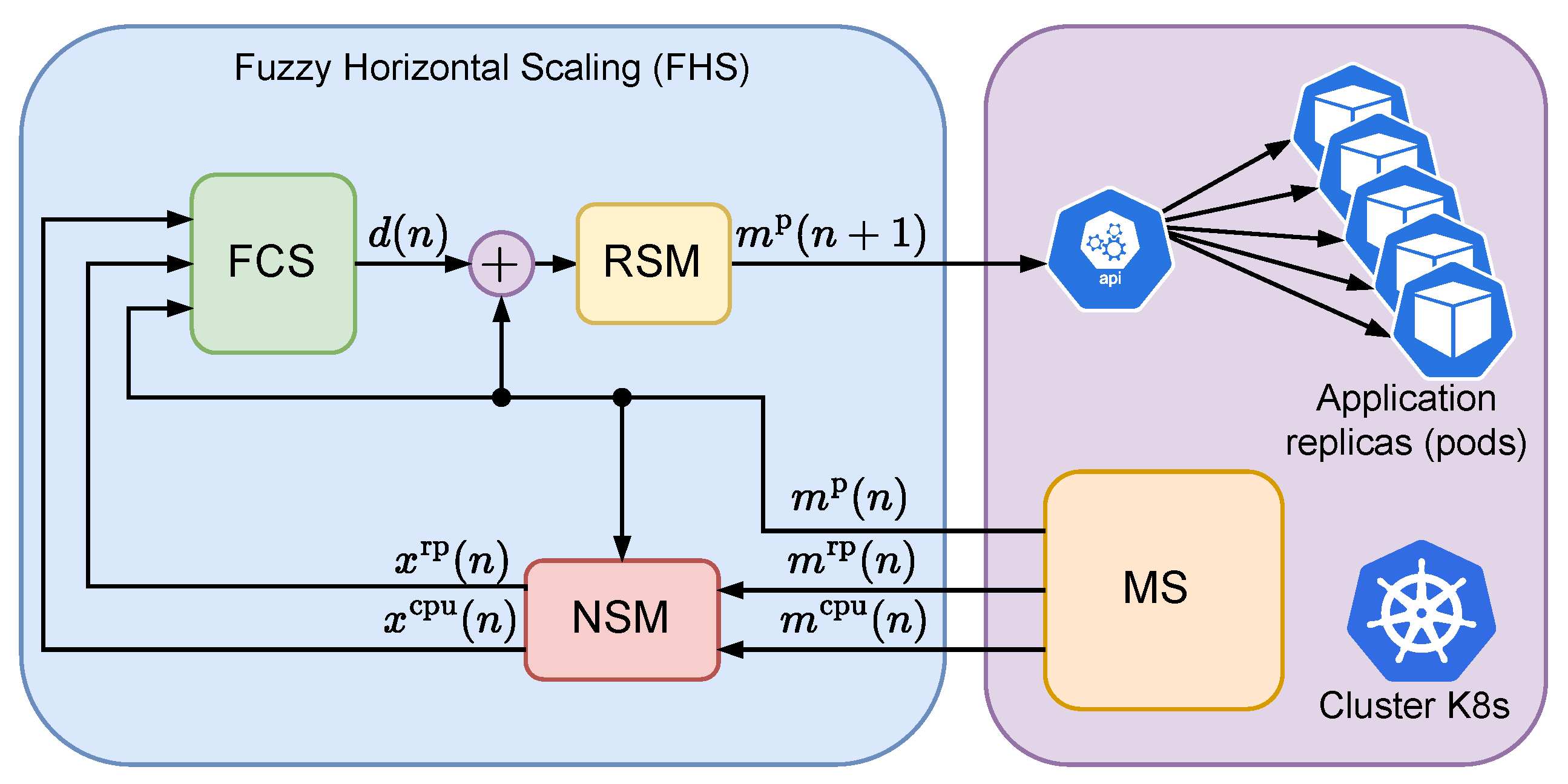
Figure 1 describes the architecture of the FHS, in which a fuzzy system, also known in the literature as a fuzzy control system (FCS), is used for horizontal scaling control of a given application in a Kubernetes cluster (K8s). At each n-th point in time, the FCS takes as input the variables , , and , respectively representing the CPU load in millicores, the rate of received packets per minute (rpm), and the number of replicas of a given application, with the first two terms normalized by the number of application replicas. The variables and are generated by a module which we call the Normalization and Saturation Module (NSM), which captures the application metrics through a Monitoring Service (MS) associated with the K8s cluster. The MS is responsible for capturing metrics related to the CPU load of all the application replicas , the rate of packets received by all the application replicas in rpm , and the number of application replicas . At every n-th moment, the FCS outputs the variable , which represents a possible increment to the number of application replicas. The increment value is added to the current number of replicas to generate the next number of replicas to be achieved by K8s. The value associated with the next number of instances, previously rounded to an integer, is then saturated using a module called the Round and Saturation Module (RSM) to produce the value , which is sent to the K8s cluster. Adjustments to the number of instances are made directly by the K8s API.
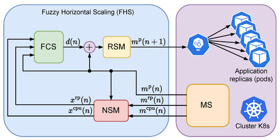
Figure 1.
Architecture of the proposed fuzzy control for horizontal scaling of applications in a Kubernetes cluster.
The variable can be expressed as follows:
where is the maximum expected load per application replica. Meanwhile, the variable can be expressed as
where is the maximum number of packets received per application replica in rpm. Finally, the variable can be expressed as follows:
where is the maximum number of instances associated with the application. The variable has an integer value between 1 and . Based on Figure 1, Equations (1) and (2) are implemented by the NSM and Equation (3) is implemented by the SM. As noted by Equations (1) and (2), the values of and are normalized between 0 and 1; meanwhile, the values of are limited between and , where K is the maximum number of increments that can be performed at each n-th moment.
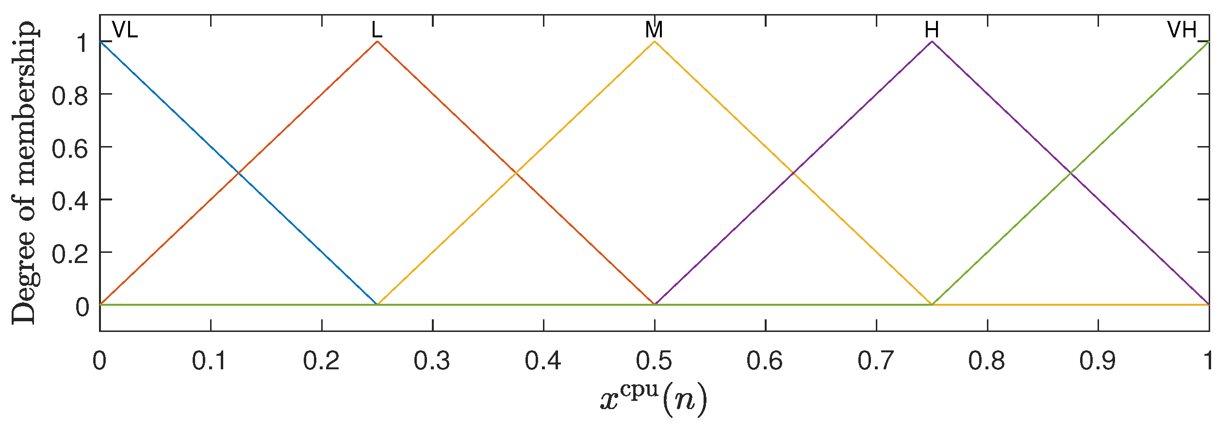
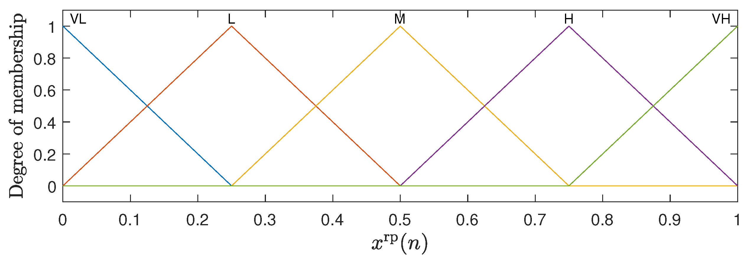
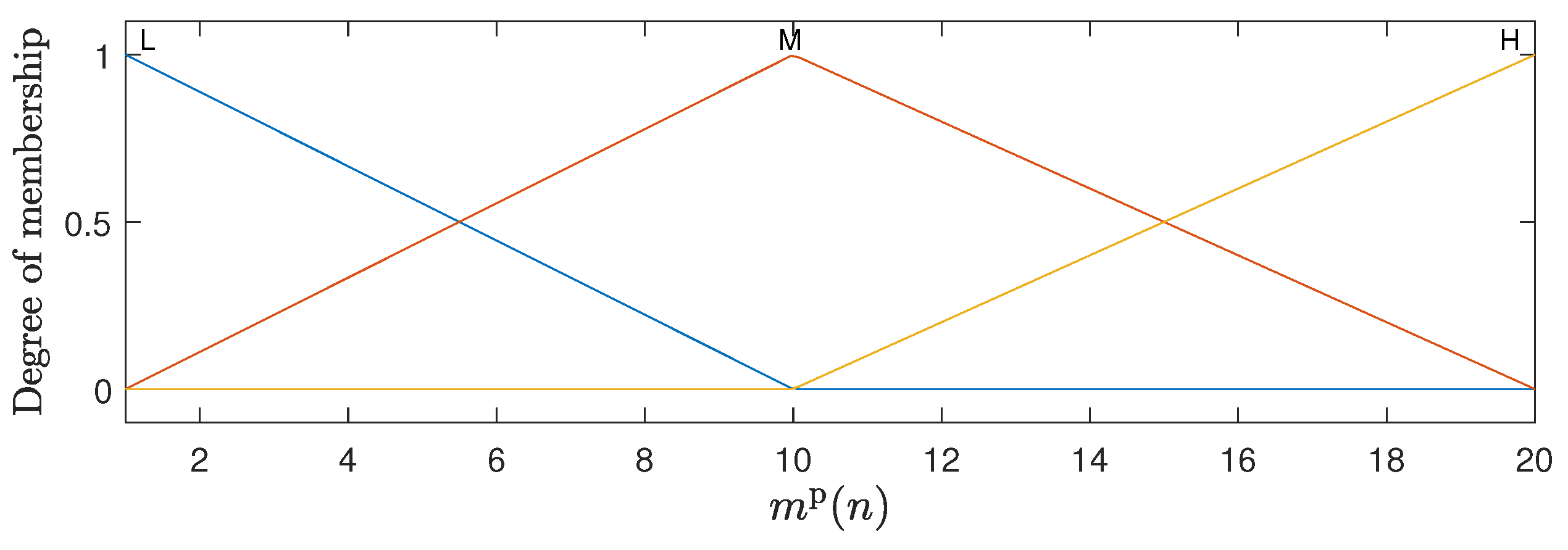
The fuzzy inference system adopted in this work is of the Mandani type, which is widely used in fuzzy control problems [20,22]. For the representation of the inputs to the fuzzy system, membership functions are defined that capture the relationship between the input values and their pertinence in each fuzzy set [20]. The inputs and both have five membership functions in the triangular form, which are uniformly distributed between 0 and 1. The input has three membership functions, with trapezoidal shapes at the ends and a triangular function in the center uniformly distributed between 1 and . The graphical representation of these membership functions can be observed in Figure 2, Figure 3 and Figure 4. For the membership functions associated with the variable , Figure 4 shows an example for .
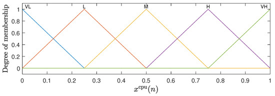
Figure 2.
Membership functions associated with the CPU load .
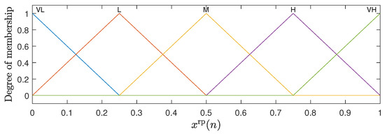
Figure 3.
Membership functions associated with the rate of received packets .
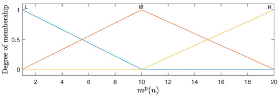
Figure 4.
Membership functions associated with the number of replicas ; in this example, .
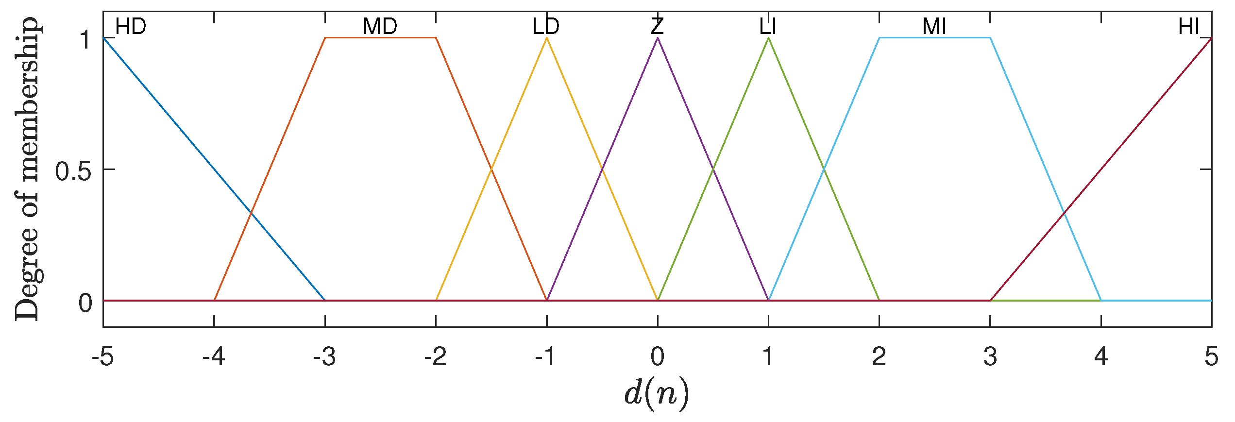
The output is represented by seven membership functions, with trapezoidal shapes at the ends and triangular functions for the rest of the interval. These membership functions represent the different possibilities for incrementing or decrementing the number of replicas of the application. Figure 5 illustrates the membership functions used for for the case where .
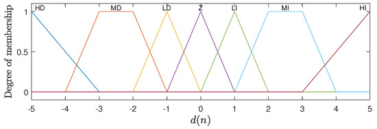
Figure 5.
Membership functions associated with the output variable representing the increase in the number of replicas of the application ().
The linguistic terms associated with the membership functions of the variables and are the same as illustrated in Figure 2 and Figure 3: Very Low (VL), Low (L), Mean (M), High (H), and Very High (VH). The variable uses the terms Low (L), Mean (M), and High (H) for its functions; see Figure 4. In the case of the output variable , the linguistic terms are High Decrement (HD), Mean Decrement (MD), Low Decrement (LD), Zero (Z), Low Increment (LI), Mean Increment (MI), and High Increment (HI). The FHS fuzzy inference machine makes use of 75 production rules, which are presented in detail in Table 1.

Table 1.
Description of the rules used by FHS.
The fuzzy decision rules used in the FHS system were carefully crafted based on expert knowledge and understanding of the system’s dynamics. These rules were designed to capture the essential behaviors and interactions within the K8s environment under various load conditions. While there are many rules, each plays a specific role in ensuring precise and responsive scaling decisions. The rules were generated through iterative testing and validation to ensure they effectively manage the load and resource allocation.
For the fuzzy inference process, we use the minimum criterion for the AND operation (implication) and the maximum criterion for generating outputs. The fuzzy rules are applied using minimum implication, where the minimum value of the inputs determines the degree of rule activation. All conditions must be met to at least the minimum degree specified in order for a rule to be activated. When the rules are activated, their outputs are combined using the maximum criterion. This aggregation step takes the maximum value from the outputs of all activated rules, ensuring that the most significant contributions are considered in the final decision-making process. Finally, the defuzzification process is performed using the centroid method, which calculates the center of mass of the resulting fuzzy set to obtain a precise output value. This output value adjusts the system’s number of replicas (pods). By employing the centroid method, the FHS system can provide a balanced and accurate representation of the fuzzy set, which translates into more precise and efficient scaling decisions. This dynamic adjustment allows the FHS to respond effectively to real-time load conditions, thereby optimizing resource usage while maintaining system performance.
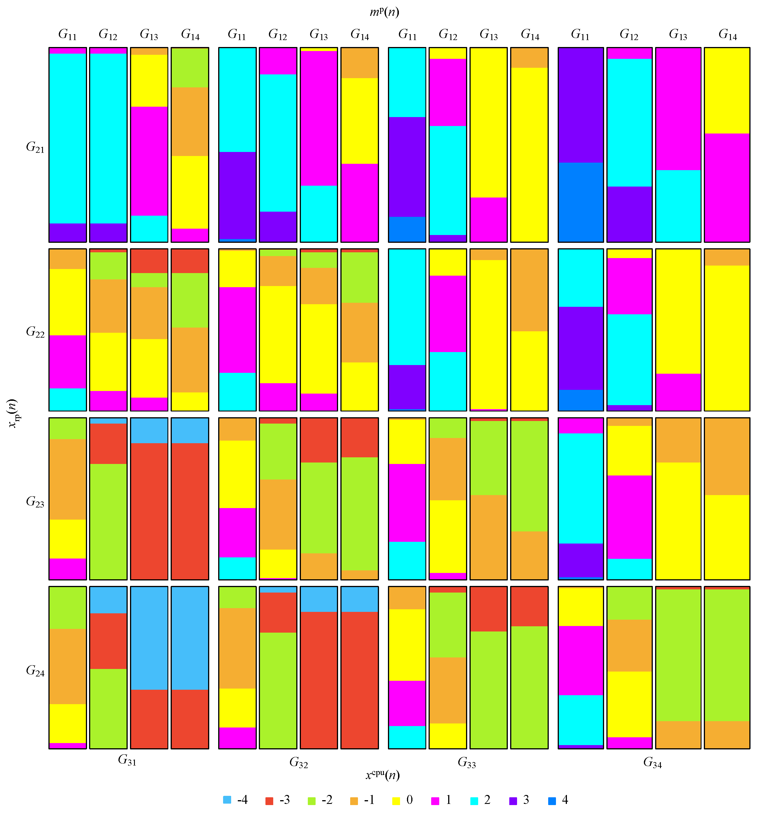
Figure 6 uses a mosaic-type diagram to illustrate the mapping between input and output of the FCS for various values; these are uniformly distributed between 0 and 1 for the variables and and between 1 and for the variable . In the figure, the value of the output variable is rounded ().

Figure 6.
Mosaic-type diagram illustrating the mapping between the input and output of the FCS.
As can be observed in Figure 6, each input variable is grouped into four groups of values, represented as , where, . Table 2 details the value of each group, where , , and .

Table 2.
Description of the values associated with the groups presented in Figure 6.
3. Methodology
The experiment consisted of the use of two distinct Virtual Machines (VMs) for different purposes [23,24,25]. The first VM was set up as a MicroK8s-type K8s cluster [26], where a web application target of the experiment was deployed. This machine acted as the target environment for testing the scaling of replicas. The second VM was dedicated to running JMeter (https://jmeter.apache.org/index.html) [27,28,29,30,31,32]. This machine was responsible for generating HTTP traffic demands to the web application hosted on the K8s cluster. The web application deployed on K8s was developed in Java using Dropwizard version 3.1 (https://www.dropwizard.io/en/stable/) [33]; it performs calculations of Fibonacci sequences of order 15 and returns this sequence as a response to the requests made by JMeter [34,35]. The application deployed on K8s was limited to 150 millicores and 256 MB. The FHS was configured to work with millicores per replica, rpm per replica, and replicas.
In addition to these virtual machines, the proposed FHS fuzzy controller for scaling of replicas was implemented and run on the experiment’s own host. Using Matlab (596681) as the development environment, FHS used the Java Fabric8 Kubernetes–Client library [36] to interact with the K8s API and perform dynamic scaling of the web application replicas. Thus, FHS acted as an external component to the cluster, making scaling decisions based on collected metrics and sending scaling requests to the Kubernetes MicroK8s cluster. Metrics were collected using Prometheus [37], which functioned as the MS (see Figure 1). The VM with the K8s cluster had 12 GB of RAM, four CPUs, and used Ubuntu 20.04 for the server, while the other VM had 12 GB of RAM, three CPUs, and used Ubuntu 22.04 for the server. The host was a machine with 128 GB of RAM and sixteen CPUs, and used Windows 10. Figure 7 illustrates the structure of the methodology used to generate the results.
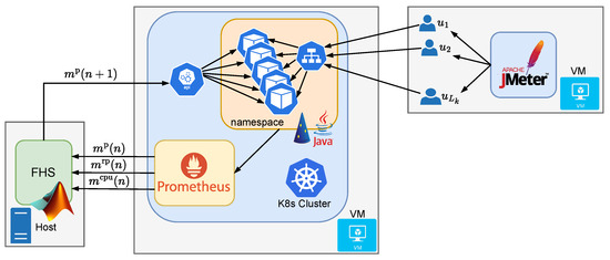
Figure 7.
Architecture of the methodology used to generate the results.
The results were generated from the load profile illustrated in Figure 8. This profile was constructed using the Open Model Thread Group, which defines the amount of virtual users created over time by JMeter to generate traffic demand on the web application being run on K8s [27]. The load profile shown in Figure 8 was chosen to simulate a realistic and variable workload scenario that reflects conditions encountered in edge computing environments. This profile includes periods of high and low demand, which allows for a comprehensive evaluation of the FHS system’s ability to adjust resources in response to changing workloads. The chosen load profile helped to test the robustness and responsiveness of the FHS system, ensuring its ability to maintain performance and efficiency under various conditions. By including a range of workload intensities, the aim was to demonstrate the system’s capability to handle peak loads efficiently while scaling down resource usage during periods of lower demand, thereby optimizing resource utilization and maintaining service quality.

Figure 8.
Profile of virtual user creation by JMeter using Open Model Thread Group for generating access to the web application.
With a duration of 180 s, the user creation load profile is characterized by a ramp-up in the first 60 s until reaching a quantity of users. Between 60 and 120 s, the requests remain constant at ; after 120 s, the number of users decreases in a ramp (following the same rate of increase) until 180 s. The number of virtual users at a given time, , can be expressed as follows:
where is the maximum number of virtual users that the load profile can reach. Tests were carried out with 30 different values for , where each k-th value can be expressed as for . The tests were repeated three times for each k-th value of , totaling 90 experiments.
The decision to use three repetitions was meticulously based on a comprehensive statistical analysis. This analysis aimed to determine whether the , , and measurements from each experiment for each k-th value were significantly different. To ensure that the correct hypothesis test was applied, the Kolmogorov–Smirnov test was initially conducted on each dataset to determine whether the distributions were normal. Checking for normality is crucial, as it determines whether the data should be analyzed using a parametric test such as ANOVA or a nonparametric test such as Kruskal–Wallis [38,39,40]. Following the Kolmogorov–Smirnov test, it was observed that all p-values were below for every experiment across all load values, indicating that the distributions of the variables analyzed (, , and ) did not follow a normal distribution. The average p-value was around , reinforcing the conclusion that the normality assumption should be rejected. Based on these results, the nonparametric Kruskal–Wallis test was chosen to assess whether there were significant differences between the repetitions of the experiments [38,39,40].
The Kruskal–Wallis test was applied to each replication experiment (, , and ) across all load values. The Kruskal–Wallis test determines whether there are statistically significant differences between the medians of two or more independent groups. It starts with the null hypothesis () that all samples come from the same distribution, meaning that there is no significant difference between the groups. In the event that the p-value from the test is lower than the significance level (), the null hypothesis is rejected, indicating that at least one of the groups has a different distribution. As the data distributions were abnormal, Kruskal–Wallis represents the appropriate choice for this type of analysis [40].
The results of the Kruskal–Wallis tests showed that the mean p-value for the variable was , with a median of and a standard deviation (std) of . For the variable, the mean p-value was with a median of and std of . Finally, for the variable, the mean p-value was with a median of and std of . Table 3 shows all of the p-value results obtained from the Kruskal–Wallis test for the variables , , and considering each value.

Table 3.
Kruskal–Wallis p-values for , , and variables across different load values.
These values, as shown in Table 3, indicate that in most cases the p-values were consistently above the threshold, suggesting no statistically significant evidence to reject the null hypothesis. The consistency of these results, as reflected in the mean values and the low variation of the p-values (std) presented in Table 3, suggests that three repetitions were sufficient to capture the variability of the data without introducing significant differences. Thus, the analysis confirms that three repetitions per experiment were adequate, validating the methodology used in this study. The decision to use three repetitions allowed for a balance between the need for statistical accuracy and the efficiency of computational resources, ensuring that the obtained conclusions are robust and reliable without the need for a greater number of repetitions, which could have unnecessarily increased the cost and execution time of the experiments. This efficient use of resources should provide confidence in the methodology’s practicality.
For comparison purposes, additional experiments were also conducted using the native Horizontal Pod Autoscaler (HPA) of K8s [1,2]. These tests followed the same approach as those with the FHS, varying the load by the number of users through the profile illustrated in Figure 8 and by Equation (4). The HPA was deployed with the parameters averageUtilization: 2, minReplicas: 1, maxReplicas: 20, scaleDown: stabilizationWindowSeconds: 0 and scaleUp: stabilizationWindowSeconds: 0.
At the end of the tests with FHS and HPA, 90 sets of data were created, with CPU load used by the application in millicores being , the rate of packets received by the application in rpm , the number of replicas , and the latency of requests made by JMeter , as associated with the i-th repetition of the k-th test of 180 seconds. It is important to note that the variables and consider all replicas running at the given time t. The variables , , and were obtained by Prometheus, while the variable was obtained by JMeter.
4. Results
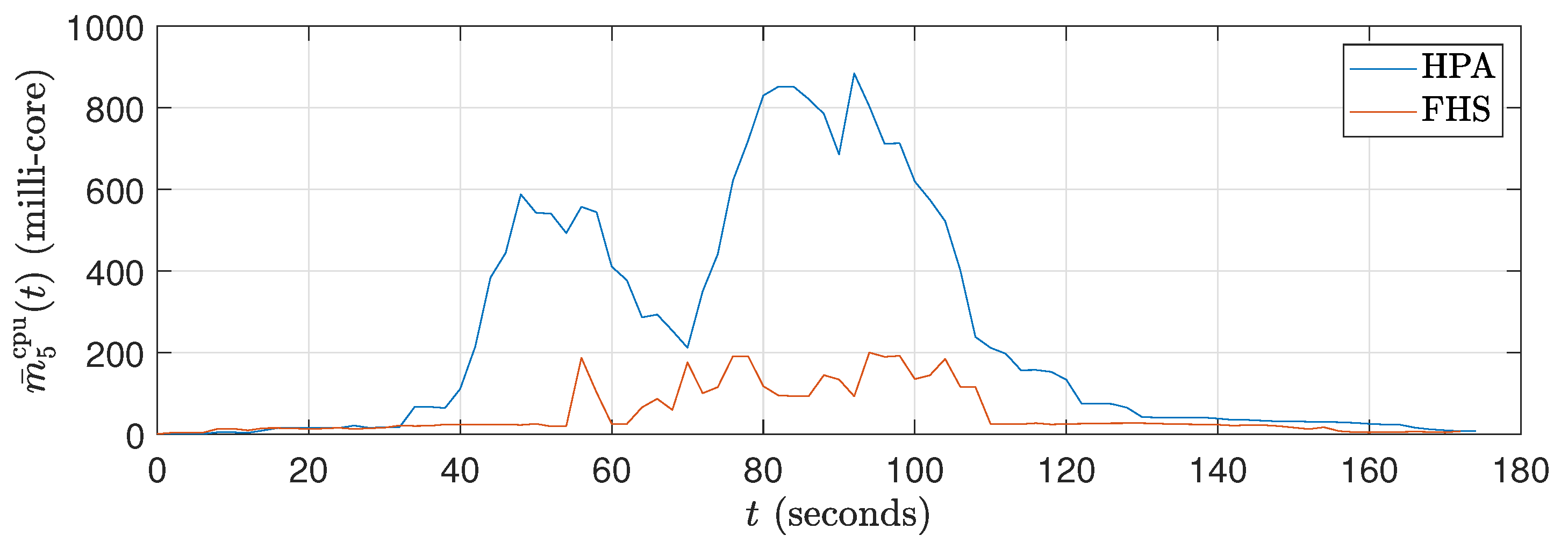
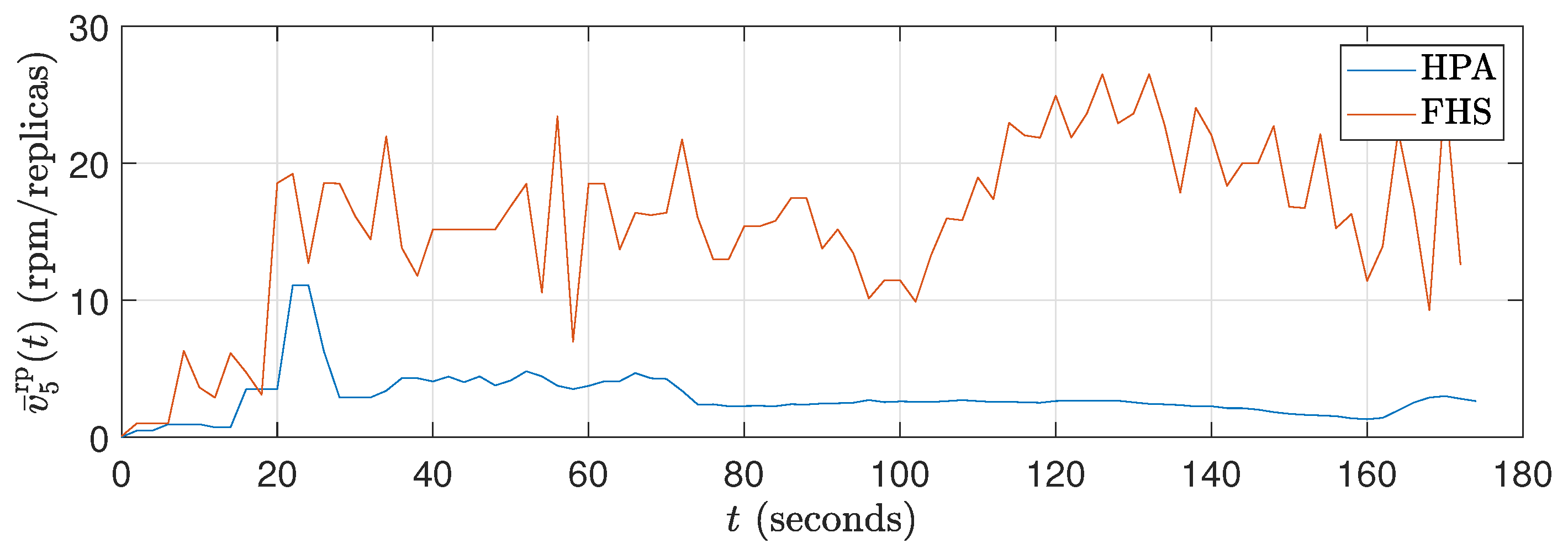
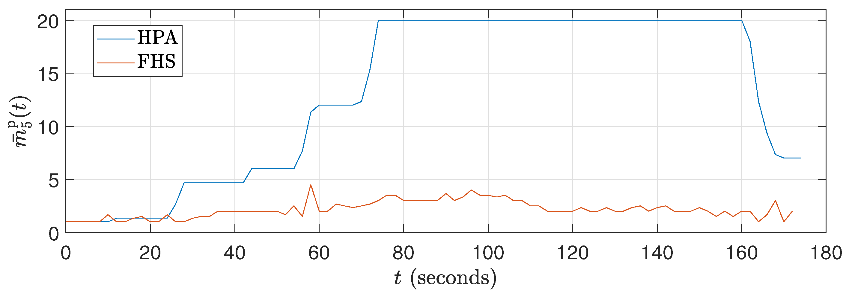
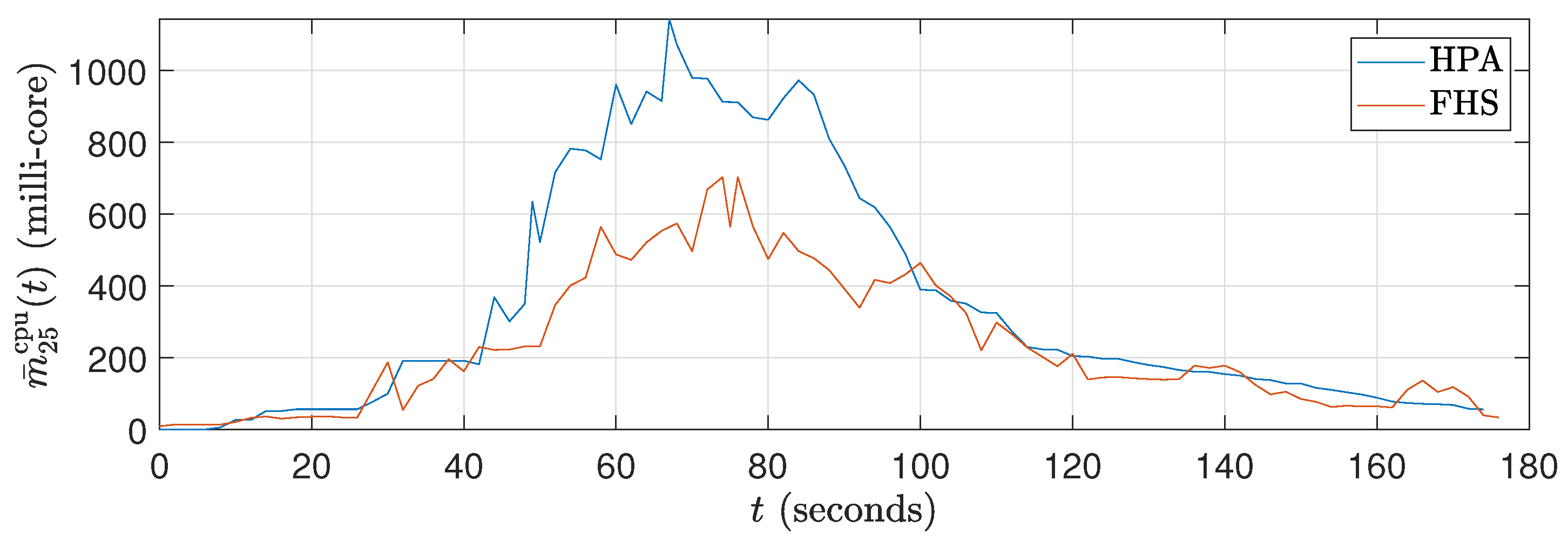
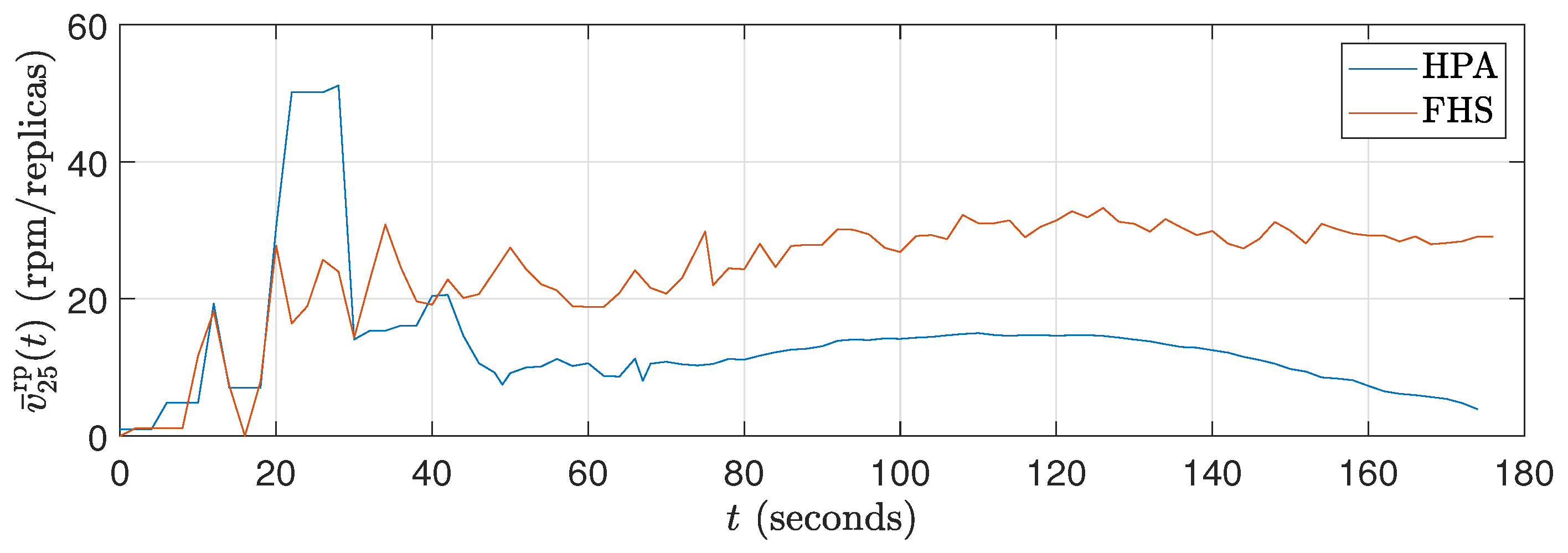
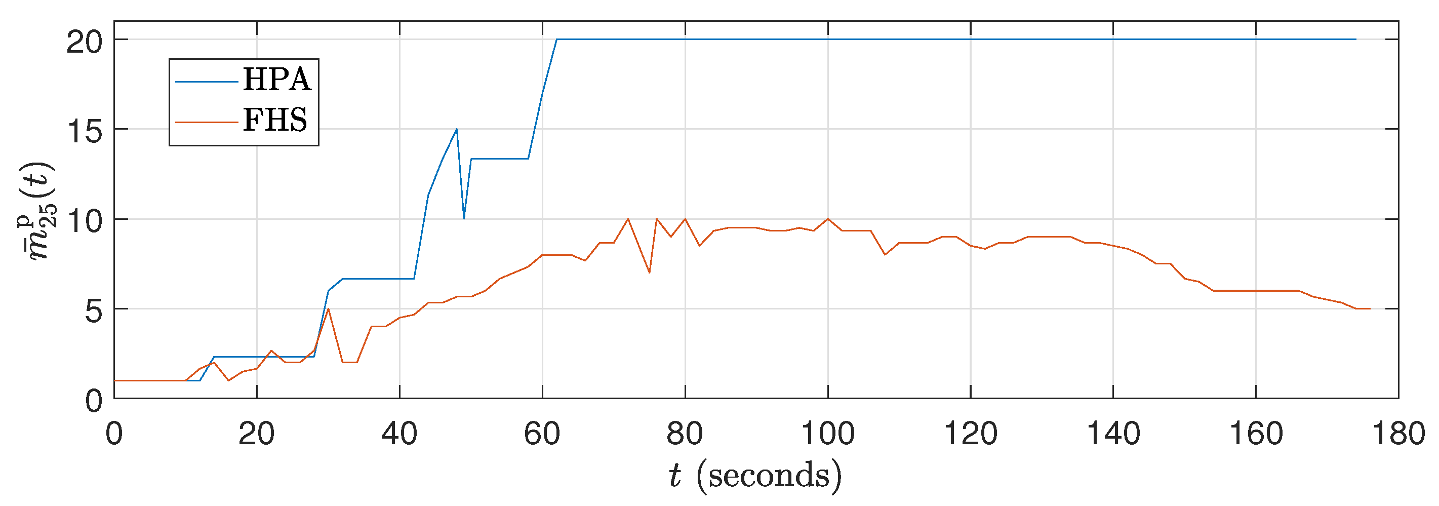
Figure 9, Figure 10, Figure 11, Figure 12, Figure 13 and Figure 14 show the average CPU consumption curves in millicores , the average packet rate per replica in rpm, and the average number of replicas over time for the experiments with () and (). In this case, the average of the three repetitions was taken for each k-th test, in which the calculation of , , and can be expressed as
and
where
in which is the rate of packets received in rpm per replica. The values and were chosen in order to illustrate the system’s performance under low and high load conditions, respectively.
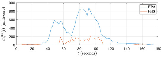
Figure 9.
Average CPU consumption curves in millicores for ().
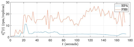
Figure 10.
Average rate of packets received in rpm curves for ().
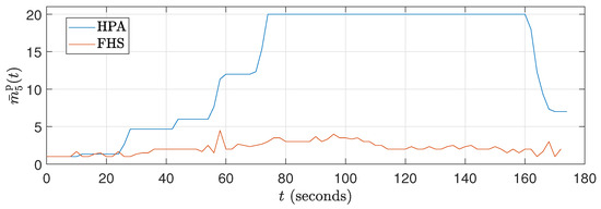
Figure 11.
Average number of replica curves for ().
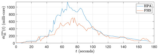
Figure 12.
Average CPU consumption curves in millicores for ().
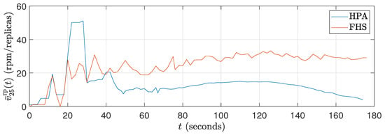
Figure 13.
Average rate of packets received in rpm curves for ().
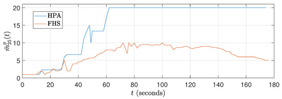
Figure 14.
Average number of replicas curves for ().
A millicore is a unit of measurement used to quantify the processing capacity of a CPU in computing systems, especially in cloud computing environments and Kubernetes. An entire CPU core is divided into a thousand equal parts, with each millicore representing one one-thousandth of a CPU core; for example, 1000 millicores is equal one entire CPU core. This granularity allows for precise allocation of CPU resources to containers or pods to ensure that each application receives the amount of processing power it needs, thereby optimizing the utilization of available hardware resources.
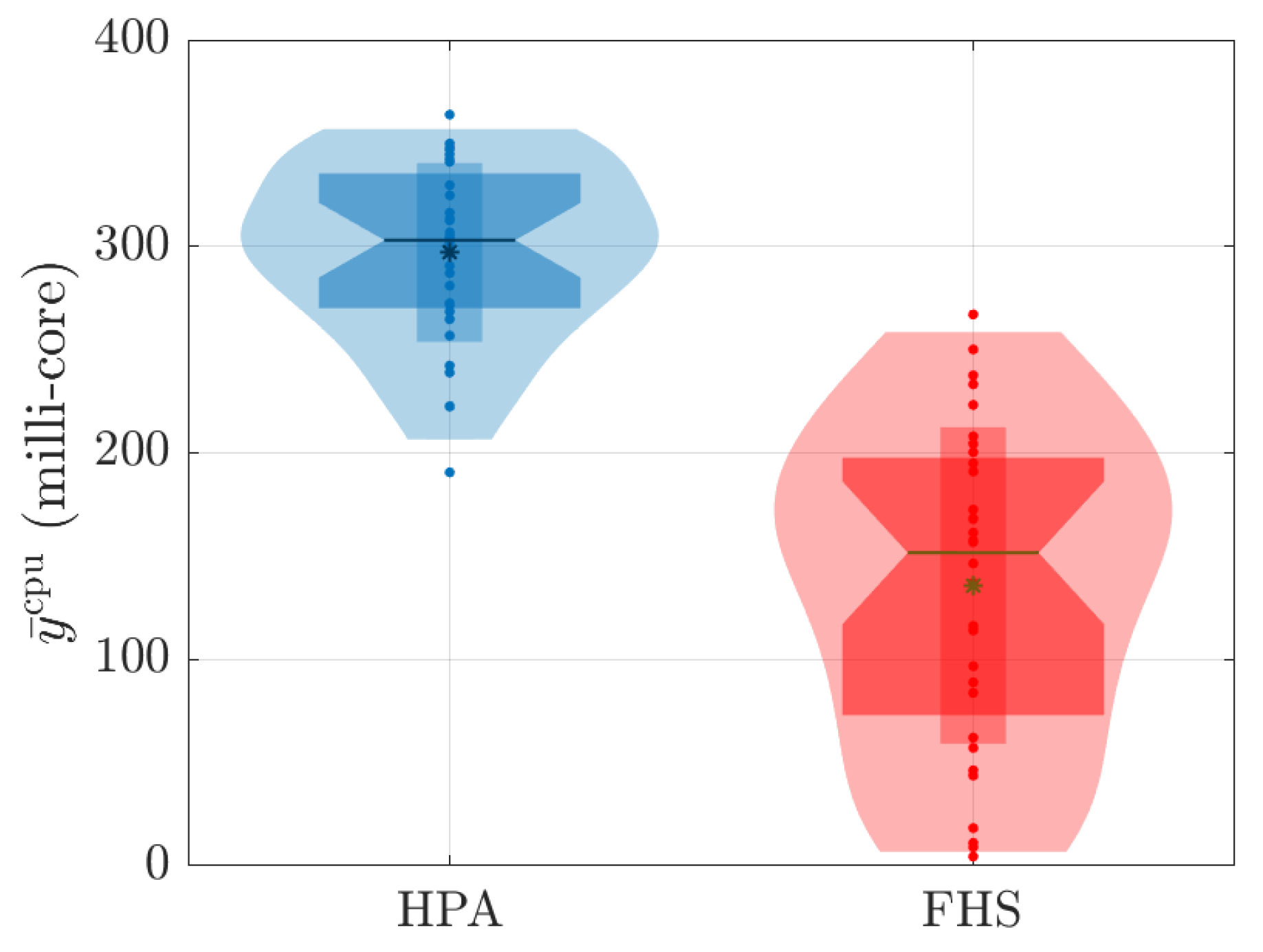
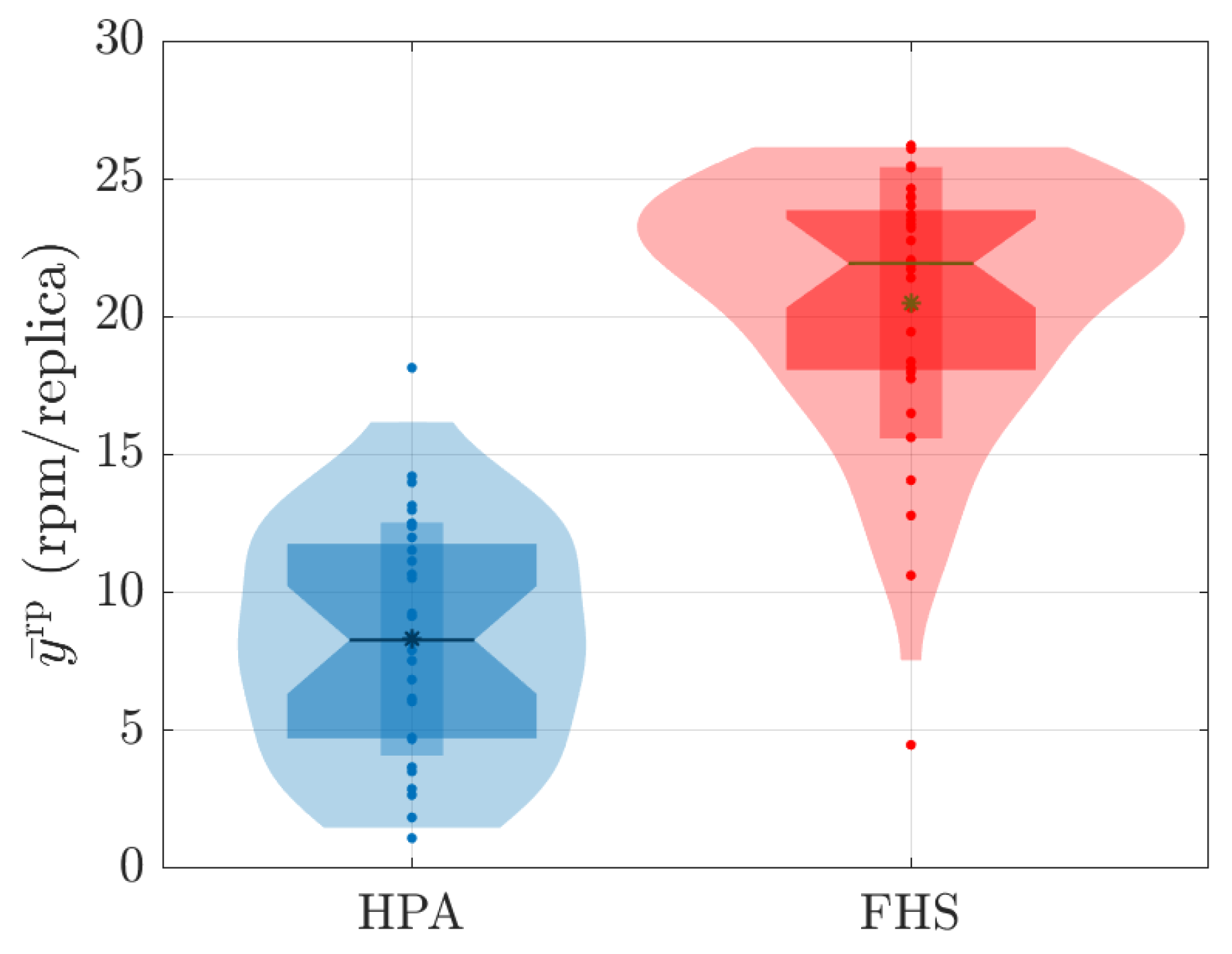
Figure 15, Figure 16 and Figure 17 show the distribution of values associated with the average metrics of CPU, received packets, and number of replicas around the 180 seconds associated with each k-th test for all values. For each k-th test, the values , , and were generated, and can be expressed as follows:
and

Figure 15.
Distribution of values associated with average CPU consumption during 180 s for all values tested.

Figure 16.
Distribution of values associated with the average rate of packets received in rpm per replicas during 180 s for all values tested.
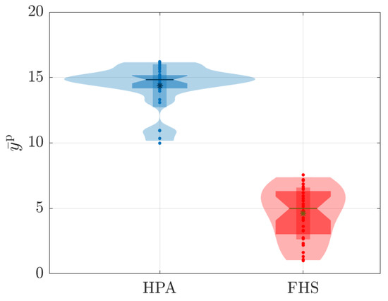
Figure 17.
Distribution of values associated with the average number of replicas during 180 s for all values tested.
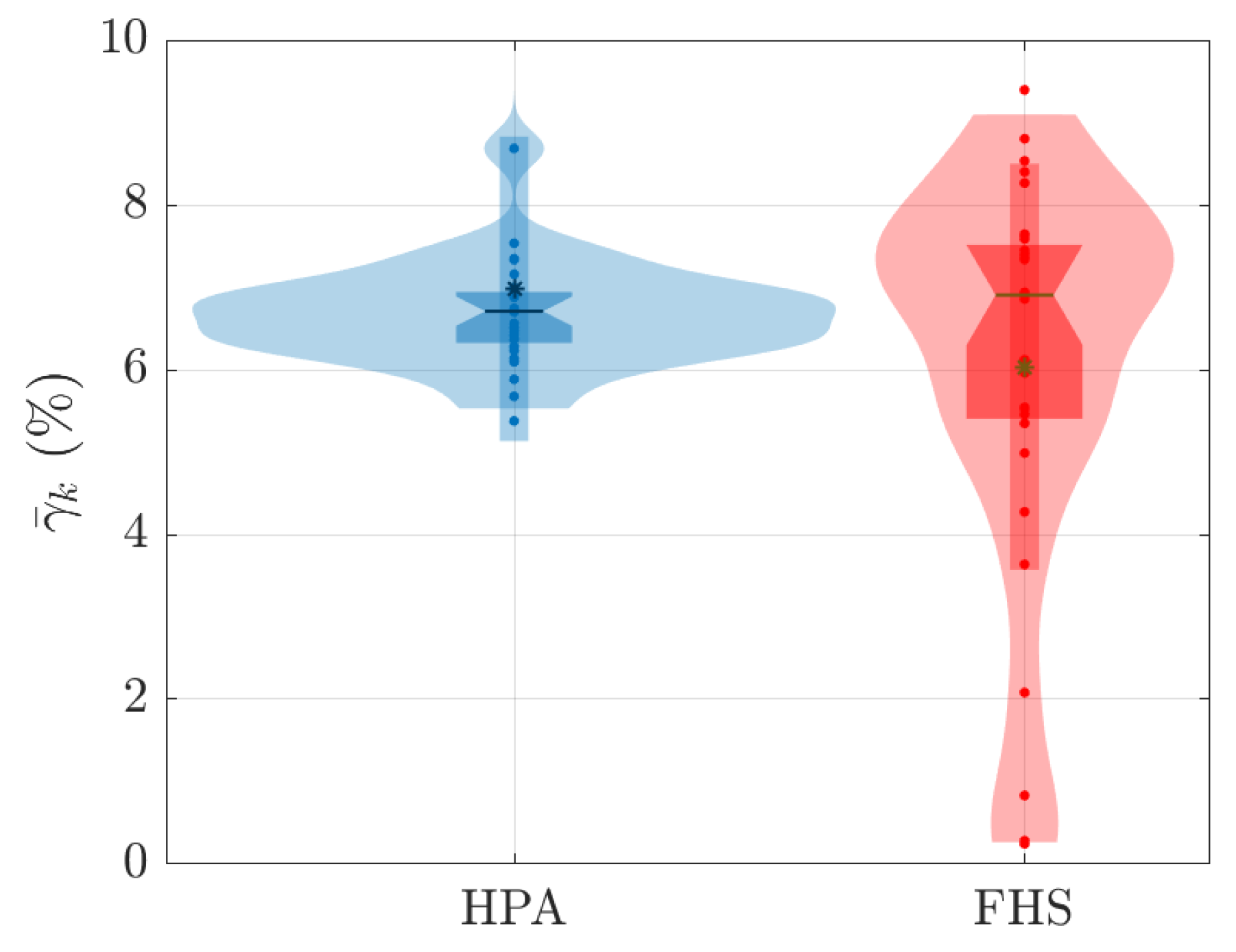
Finally, Figure 18 presents the data distribution of the average rate of violation for a predetermined latency SLA , characterized here as [10]. The latency SLA violation rate for each i-th repetition associated with the k-th test was calculated based on the latency measures of the HTTP requests made by JMeter, i.e.,
where is the number of requests made by JMeter in the i-th repetition of the k-th test and can be expressed as
where is the latency of the j-th request of the i-th repetition associated with the k-th test. Based on the values of , the average associated with the SLA violation rate for each k-th test was calculated as follows:
Figure 18 presents the results for ms.

Figure 18.
Distribution of the average associated with the violation rate for a latency SLA of ms.
5. Analysis of Results
The obtained results demonstrate that FHS presents advantages over Kubernetes’ HPA, especially regarding customization and reduction of the required number of replicas. During the 90 experiments we carried out with different stress scenarios (different values) generated by JMeter, it was observed that FHS managed to maintain a lower CPU consumption compared to HPA. Figure 9 and Figure 12 illustrate these results during the 180 s of two specific tests ( and ), and Figure 15 reinforces this result for all tests conducted.
Figure 9 shows that the CPU consumption of HPA is higher because it significantly increases the number of replicas to 120 s, resulting in a peak CPU load. This peak occurs because the workload profile is at its maximum between approximately 40 seconds and 120 seconds. With more replicas (see Figure 11), HPA exhibits greater CPU consumption. On the other hand, Figure 9 reveals that the packet reception rate per replica is reduced in HPA due to the higher number of replicas. In contrast, FHS, which uses fewer replicas, results in lower CPU consumption and a higher packet reception rate per replica, as shown in Figure 9, Figure 10 and Figure 11.
In Figure 12, it can be observed that the CPU consumption of HPA is significantly higher due to the rapid increase in replicas up to 120 seconds, resulting in peak CPU load. This behavior results from the workload profile, which is at its maximum between approximately 40 s and 120 s. With a higher number of replicas, HPA shows increased CPU consumption. In contrast, Figure 13 shows that the packet reception rate per replica is lower in HPA due to the large number of replicas (see Figure 14). On the other hand, FHS uses fewer replicas, resulting in lower CPU consumption and a higher packet reception rate per replica. Figure 12 highlights that while the workload decreases after 120 s, the number of replicas in HPA does not decrease at the same rate, maintaining higher CPU consumption for a more extended period. This behavior underscores the efficiency of FHS in dynamically adjusting the number of replicas to provide more balanced and efficient resource utilization over time.
Although the workload decreases after 120 s, the number of replicas in HPA does not decrease at the same rate, allowing higher CPU consumption to be maintained for a more extended period. In contrast, FHS dynamically adjusts the number of replicas more efficiently, resulting in more balanced and efficient resource consumption over time. This difference in behavior between HPA and FHS highlights the ability of FHS to manage resources more effectively, ensuring better CPU utilization and higher efficiency in packet delivery per replica and validating its application in real-world edge computing scenarios.
The fact that FHS uses a smaller number of replicas compared to HPA in all experiments contributes to the reduction in CPU rate. With fewer replicas in operation, the workload is distributed more efficiently among them, resulting in lower CPU consumption per replica. This indicates better utilization of available resources and a reduction in system overhead. This feature can be advantageous in stress scenarios, as it allows for more precise optimization and a better balance between resource demand and system capacity. Figure 11 and Figure 14 illustrate these results during the 180 s of two specific tests ( and ). Meanwhile, Figure 17 details this result for all the tests conducted.
As shown in Figure 10, Figure 13, and Figure 16, FHS results in a higher packets rate in rpm per replica compared to HPA. This difference indicates that HPA tends to underutilize the replicas, as it allocates a larger number of them compared to FHS to meet the same stress demand (different values).
Regarding the violation rate of the latency SLA of 250 ms, it is interesting to note that the results in Figure 18 show significant differences between HPA and FHS. While HPA presents values concentrated around and violation, FHS exhibits a broader distribution ranging from to violation. This indicates that FHS was able to deal more efficiently with load variation and demand, adapting the number of replicas more appropriately to keep latency levels within the limit established by the SLA.
The ability to adjust the number of replicas more precisely and efficiently is one of the main benefits of FHS. By analyzing the workload, received packet rate, and number of pods or replicas, FHS applies customized fuzzy rules to determine the ideal number of replicas needed to meet the demand, thereby avoiding excessive resource allocation. This results in better utilization of available resources in K8s. The improved customization and finer adjustment capability of FHS can contribute to a better user experience and ensure improved service quality.
6. Comparison with State of the Art
The FHS system advances the state of the art by explicitly integrating edge computing into the autoscaling process. Unlike the RL-based methods proposed in [3,7,10], which primarily focus on cloud-centric environments, FHS is tailored for Kubernetes environments that simulate edge computing scenarios. This integration reduces latency and optimizes resource usage closer to the data source, providing significant advantages for innovative city applications. Moreover, RL-based autoscaling requires complex training phases and substantial computational resources, whereas FHS offers a more straightforward implementation with immediate applicability. In addition, it is independent of extensive historical data, making it more suitable for real-time edge computing environments where data are often dynamic and unpredictable.
In [17], the authors proposed a Kubernetes scaling engine leveraging various ML forecasting methods to manage dynamic incoming requests. Although these ML-based approaches provide sophisticated scaling predictions, they require complex setups and ongoing computational power in order to maintain accuracy. Conversely, the FHS system employs fuzzy logic, offering a more straightforward implementation with immediate applicability. It also avoids reliance on extensive historical data, making it more practical for real-time edge computing scenarios where data can be highly dynamic and less predictable.
The FHS system offers several advantages over the fuzzy logic-based autoscaling approach presented in [19], which proposed a self-adaptive cluster architecture for lightweight edge devices utilizing fuzzy logic within a serverless framework implemented on a cluster of Raspberry Pi devices. In contrast, the proposed FHS system is designed for Kubernetes environments, simulating real-time edge computing scenarios. This approach reduces latency and optimizes resource usage near the data source, which is beneficial for applications where data are frequently dynamic, such as in smart city contexts. The fuzzy logic in FHS allows for a more straightforward implementation without extensive training or dependence on large historical datasets. While the work in [19] focused on serverless functions and static configurations, FHS adapts to dynamic edge computing scenarios, handling varied workloads and offering a scalable solution for computing infrastructures.
The FHS system also surpasses the fuzzy logic-based auto-scaling approach proposed in [18], which dynamically adjusts thresholds and cluster size for web applications in the cloud, aiming to reduce resource consumption without violating SLAs. This approach focuses on vertical scaling in cloud environments and needs to address the challenges of edge computing, where latency and data proximity are crucial. The proposed FHS system is designed for Kubernetes environments simulating real-time edge computing, focusing on horizontal scaling. This helps reduce latency and optimize resource usage near the data source.
7. Conclusions
The FHS system proves to be an efficient approach for horizontal replica scaling in Kubernetes environments, especially in the context of edge computing. By using fuzzy logic, FHS dynamically adjusts the number of replicas, thereby reducing CPU consumption and requiring fewer replicas to meet load demands. Our experimental results show that FHS outperforms the standard Kubernetes HPA scaling mechanism regarding resource consumption and maintaining SLAs, demonstrating its capability to handle dynamic and unpredictable scenarios typical of edge computing. Furthermore, the ability of FHS to operate without requiring large historical datasets or extensive training phases makes it a practical and applicable solution for various applications. The integration of edge computing enables optimization of resource usage close to the data source, thereby reducing latency and improving operational efficiency. These characteristics make FHS a scalable tool for next-generation computing infrastructure, potentially benefiting intelligent city applications and areas such as connected healthcare, autonomous vehicles, and smart factories in which real-time computing and resource optimization are essential.
A limitation of the FHS system is related to the precise definition of fuzzy rules and control parameters. Fuzzy systems require manual configuration of rules based on specialized domain knowledge, which can be time consuming and prone to error. Additionally, adjusting these parameters to achieve optimal performance can be a complex and iterative process that does not guarantee the system’s generalization to different operational conditions. A promising future approach for this work could be the implementation of machine learning techniques for the automatic definition and adjustment of fuzzy rules. Such integration would significantly improve the system’s efficiency and accuracy, allowing for dynamic adaptation to changing operational conditions. Consequently, the reduced need for manual intervention would make the system more robust and autonomous.
Author Contributions
All authors have contributed in various degrees to ensure the quality of this work. S.N.S. and M.A.C.F. conceived the idea and experiments; S.N.S. and M.A.C.F. designed and performed the experiments; S.N.S., M.A.S.d.S.G., L.M.D.d.S. and M.A.C.F. analyzed the data; S.N.S., M.A.S.d.S.G., L.M.D.d.S. and M.A.C.F. wrote the paper; and M.A.C.F. coordinated the project. All authors have read and agreed to the published version of the manuscript.
Funding
Coordenação de Aperfeiçoamento de Pessoal de Nível Superior—Brasil (CAPES)—Finance Code 001.
Data Availability Statement
The raw data supporting the conclusions of this article will be made available by the authors on request. The data are not publicly available due to privacy concerns and the sensitive nature of the data used in the experiments, which may include proprietary information and detailed configuration of the infrastructure setup used in the study.
Acknowledgments
The authors would like to express their gratitude to the Coordenação de Aperfeiçoamento de Pessoal de Nível Superior (CAPES) for providing financial support.
Conflicts of Interest
The authors declare no conflicts of interest.
References
- Tran, M.N.; Vu, D.D.; Kim, Y. A Survey of Autoscaling in Kubernetes. In Proceedings of the 2022 Thirteenth International Conference on Ubiquitous and Future Networks (ICUFN), Barcelona, Spain, 5–8 July 2022; IEEE: New York, NY, USA, 2022; pp. 263–265. [Google Scholar]
- Huo, Q.; Li, S.; Xie, Y.; Li, Z. Horizontal Pod Autoscaling based on Kubernetes with Fast Response and Slow Shrinkage. In Proceedings of the 2022 International Conference on Artificial Intelligence, Information Processing and Cloud Computing (AIIPCC), Kunming, China, 21–23 June 2022; IEEE: New York, NY, USA, 2022; pp. 203–206. [Google Scholar]
- Zafeiropoulos, A.; Fotopoulou, E.; Filinis, N.; Papavassiliou, S. Reinforcement learning-assisted autoscaling mechanisms for serverless computing platforms. Simul. Modell. Pract. Theory 2022, 116, 102461. [Google Scholar] [CrossRef]
- Yao, A.; Jiang, F.; Li, X.; Dong, C.; Xu, J.; Xu, Y.; Li, G.; Liu, X. A novel security framework for edge computing based uav delivery system. In Proceedings of the 2021 IEEE 20th International Conference on Trust, Security and Privacy in Computing and Communications (TrustCom), Shenyang, China, 20–22 October 2021; IEEE: New York, NY, USA, 2021; pp. 1031–1038. [Google Scholar]
- Silva, S.N.; da Silva, L.M.; Fernandes, M.A. Lógica Fuzzy Aplicada a Escalonamento Horizontal. In Proceedings of the Anais Estendidos do XIII Simpósio Brasileiro de Engenharia de Sistemas Computacionais, Porto Alegre, Brazil, 21–24 November 2023; SBC: Porto Alegre, Brazil, 2023; pp. 13–18. [Google Scholar]
- Tari, M.; Ghobaei-Arani, M.; Pouramini, J.; Ghorbian, M. Auto-scaling mechanisms in serverless computing: A comprehensive review. Comput. Sci. Rev. 2024, 53, 100650. [Google Scholar] [CrossRef]
- Abdel Khaleq, A.; Ra, I. Intelligent microservices autoscaling module using reinforcement learning. Clust. Comput. 2023, 26, 2789–2800. [Google Scholar] [CrossRef]
- Khaleq, A.A.; Ra, I. Development of QoS-aware agents with reinforcement learning for autoscaling of microservices on the cloud. In Proceedings of the 2021 IEEE International Conference on Autonomic Computing and Self-Organizing Systems Companion (ACSOS-C), Washington, DC, USA, 27 September–1 October 2021; pp. 13–19. [Google Scholar] [CrossRef]
- Sami, H.; Otrok, H.; Bentahar, J.; Mourad, A. AI-based resource provisioning of IoE services in 6G: A deep reinforcement learning approach. IEEE Trans. Netw. Serv. Manag. 2021, 18, 3527–3540. [Google Scholar] [CrossRef]
- Xiao, Z.; Hu, S. DScaler: A Horizontal Autoscaler of Microservice Based on Deep Reinforcement Learning. In Proceedings of the 2022 23rd Asia-Pacific Network Operations and Management Symposium (APNOMS), Takamatsu, Japan, 28–30 September 2022; pp. 1–6. [Google Scholar] [CrossRef]
- Santos, J.; Wauters, T.; Volckaert, B.; Turck, F.D. gym-hpa: Efficient Auto-Scaling via Reinforcement Learning for Complex Microservice-based Applications in Kubernetes. In Proceedings of the NOMS 2023—2023 IEEE/IFIP Network Operations and Management Symposium, Miami, FL, USA, 8–12 May 2023; pp. 1–9. [Google Scholar] [CrossRef]
- Mondal, S.K.; Wu, X.; Kabir, H.M.D.; Dai, H.N.; Ni, K.; Yuan, H.; Wang, T. Toward Optimal Load Prediction and Customizable Autoscaling Scheme for Kubernetes. Mathematics 2023, 11, 2675. [Google Scholar] [CrossRef]
- Dogani, J.; Khunjush, F.; Seydali, M. K-AGRUED: A Container Autoscaling Technique for Cloud-based Web Applications in Kubernetes Using Attention-based GRU Encoder-Decoder. J. Grid Comput. 2022, 20, 40. [Google Scholar] [CrossRef]
- Mudvari, A.; Makris, N.; Tassiulas, L. ML-driven scaling of 5G Cloud-Native RANs. In Proceedings of the 2021 IEEE Global Communications Conference (GLOBECOM), Madrid, Spain, 7–11 December 2021; pp. 1–6. [Google Scholar] [CrossRef]
- Shim, S.; Dhokariya, A.; Doshi, D.; Upadhye, S.; Patwari, V.; Park, J.Y. Predictive Auto-scaler for Kubernetes Cloud. In Proceedings of the 2023 IEEE International Systems Conference (SysCon), Vancouver, BC, Canada, 7–20 April 2023; pp. 1–8. [Google Scholar] [CrossRef]
- Kakade, S.; Abbigeri, G.; Prabhu, O.; Dalwayi, A.; G, N.; Patil, S.P.; Sunag, B. Proactive Horizontal Pod Autoscaling in Kubernetes using Bi-LSTM. In Proceedings of the 2023 IEEE International Conference on Contemporary Computing and Communications (InC4), Bangalore, India, 21–22 April 2023; Volume 1, pp. 1–5. [Google Scholar] [CrossRef]
- Toka, L.; Dobreff, G.; Fodor, B.; Sonkoly, B. Machine Learning-Based Scaling Management for Kubernetes Edge Clusters. IEEE Trans. Netw. Serv. Manag. 2021, 18, 958–972. [Google Scholar] [CrossRef]
- Liu, B.; Buyya, R.; Nadjaran Toosi, A. A Fuzzy-Based Auto-scaler for Web Applications in Cloud Computing Environments. In Lecture Notes in Computer Science, Proceedings of the Service-Oriented Computing, Hangzhou, China, 12–15 November 2018; Pahl, C., Vukovic, M., Yin, J., Yu, Q., Eds.; Springer: Cham, Switzerland, 2018; pp. 797–811. [Google Scholar] [CrossRef]
- Gand, F.; Fronza, I.; El Ioini, N.; Barzegar, H.R.; Azimi, S.; Pahl, C. A Fuzzy Controller for Self-adaptive Lightweight Edge Container Orchestration. In Proceedings of the 10th International Conference on Cloud Computing and Services Science—CLOSER, Prague, Czech Republic, 7–9 May 2020; INSTICC: Rua dos Lusíadas, Portugal; SciTePress: Setubal, Portugal, 2020; pp. 79–90. [Google Scholar] [CrossRef]
- Ojha, V.; Abraham, A.; Snášel, V. Heuristic design of fuzzy inference systems: A review of three decades of research. Eng. Appl. Artif. Intell. 2019, 85, 845–864. [Google Scholar] [CrossRef]
- Chopra, P.; Gupta, M. Fuzzy Logic and ANN in an Artificial Intelligent Cloud: A Comparative Study. In Lecture Notes on Data Engineering and Communications Technologies, Proceedings of the Intelligent Communication Technologies and Virtual Mobile Networks, Tirunelveli, India, 16–17 February 2023; Rajakumar, G., Du, K.L., Rocha, Á., Eds.; Springer: Singapore, 2023; pp. 559–570. [Google Scholar]
- Radwan, A.M.; Ellabib, I.M. Fuzzy Inference Systems for Load Balancing of Wireless Networks. In Proceedings of the 2023 IEEE 3rd International Maghreb Meeting of the Conference on Sciences and Techniques of Automatic Control and Computer Engineering (MI-STA), Benghazi, Libya, 21–23 May 2023; pp. 154–158. [Google Scholar] [CrossRef]
- Jian, C.; Bao, L.; Zhang, M. A high-efficiency learning model for virtual machine placement in mobile edge computing. Clust. Comput. 2022, 25, 3051–3066. [Google Scholar] [CrossRef]
- Zhang, J.; Deng, C.; Zheng, P.; Xu, X.; Ma, Z. Development of an edge computing-based cyber-physical machine tool. Rob. Comput.-Integr. Manuf. 2021, 67, 102042. [Google Scholar] [CrossRef]
- Alnoman, A. Machine learning-based task clustering for enhanced virtual machine utilization in edge computing. In Proceedings of the 2020 IEEE Canadian Conference on Electrical and Computer Engineering (CCECE), London, ON, Canada, 30 August–2 September 2020; IEEE: New York, NY, USA, 2020; pp. 1–4. [Google Scholar]
- MicroK8s: Lightweight Kubernetes. Available online: https://microk8s.io/ (accessed on 18 July 2023).
- The Apache Software Foundation. Apache JMeter. 2023. Available online: https://jmeter.apache.org/ (accessed on 18 July 2023).
- Elkhatib, Y.; Poyato, J.P. An Evaluation of Service Mesh Frameworks for Edge Systems. In Proceedings of the 6th International Workshop on Edge Systems, Analytics and Networking, Melbourne, Australia, 23 October 2023; pp. 19–24. [Google Scholar]
- Kabamba, H.M.; Khouzam, M.; Dagenais, M.R. Vnode: Low-Overhead Transparent Tracing of Node. js-Based Microservice Architectures. Future Internet 2023, 16, 13. [Google Scholar] [CrossRef]
- Calsin Quinto, E.R.; Sullon, A.A.; Huanca Torres, F.A. Reference Method for Load Balancing in Web Services with REST Topology Using Edge Route Tools. In Lecture Notes in Networks and Systems, Proceedings of the Sixth International Congress on Information and Communication Technology: ICICT 2021, London, UK, 25–26 February 2021; Springer: Singapore, 2021; Volume 4, pp. 829–843. [Google Scholar]
- Palade, A.; Kazmi, A.; Clarke, S. An evaluation of open source serverless computing frameworks support at the edge. In Proceedings of the 2019 IEEE World Congress on Services (SERVICES), Milan, Italy, 8–13 July 2019; IEEE: New York, NY, USA, 2019; Volume 2642, pp. 206–211. [Google Scholar]
- Lenka, R.K.; Mamgain, S.; Kumar, S.; Barik, R.K. Performance analysis of automated testing tools: JMeter and TestComplete. In Proceedings of the 2018 International Conference on Advances in Computing, Communication Control and Networking (ICACCCN), Greater Noida, India, 12–13 October 2018; IEEE: New York, NY, USA, 2018; pp. 399–407. [Google Scholar]
- Dropwizard Development Team. Dropwizard. 2023. Available online: https://www.dropwizard.io/ (accessed on 18 July 2023).
- Shukla, S.; Jha, P.K.; Ray, K.C. An energy-efficient single-cycle RV32I microprocessor for edge computing applications. Integration 2023, 88, 233–240. [Google Scholar] [CrossRef]
- Hansson, G. Computation Offloading of 5G Devices at the Edge Using WebAssembly. Master’s Thesis, Lulea University of Technology, Lulea, Switzerland, 2021. [Google Scholar]
- Red Hat. Fabric8 Kubernetes-Client. 2023. Available online: https://github.com/fabric8io/kubernetes-client (accessed on 18 July 2023).
- The Prometheus Authors. Prometheus. 2023. Available online: https://prometheus.io/ (accessed on 18 July 2023).
- Cardoso, D.O.; Galeno, T.D. Online evaluation of the Kolmogorov-Smirnov test on arbitrarily large samples. J. Comput. Sci. 2023, 67, 101959. [Google Scholar] [CrossRef]
- Stoker, P.; Tian, G.; Kim, J.Y. Analysis of variance (ANOVA). In Basic Quantitative Research Methods for Urban Planners; Routledge: London, UK, 2020; pp. 197–219. [Google Scholar]
- Johnson, R.W. Alternate forms of the one-way ANOVA F and Kruskal-Wallis test statistics. J. Stat. Data Sci. Educ. 2022, 30, 82–85. [Google Scholar] [CrossRef]
Disclaimer/Publisher’s Note: The statements, opinions and data contained in all publications are solely those of the individual author(s) and contributor(s) and not of MDPI and/or the editor(s). MDPI and/or the editor(s) disclaim responsibility for any injury to people or property resulting from any ideas, methods, instructions or products referred to in the content. |
© 2024 by the authors. Licensee MDPI, Basel, Switzerland. This article is an open access article distributed under the terms and conditions of the Creative Commons Attribution (CC BY) license (https://creativecommons.org/licenses/by/4.0/).

