Abstract
There is a growing interest in high-altitude platform stations (HAPSs) as potential telecommunication infrastructures in the stratosphere, providing direct communication services to ground-based smartphones. Enhanced coverage and capacity can be realized in HAPSs by adopting multicell configurations. To improve the communication quality, previous studies have investigated methods based on search algorithms, such as genetic algorithms (GAs), which dynamically optimize antenna parameters. However, these methods face hurdles in swiftly adapting to sudden distribution shifts from natural disasters or major events due to their high computational requirements. Moreover, they do not utilize the previous optimization results, which require calculations each time. This study introduces a novel optimization approach based on a neural network (NN) model that is trained on GA solutions. The simple model is easy to implement and allows for instantaneous adaptation to unexpected distribution changes. However, the NN faces the difficulty of capturing the dependencies among neighboring cells. To address the problem, a classifier chain (CC), which chains multiple classifiers to learn output relationships, is integrated into the NN. However, the performance of the CC depends on the output sequence. Therefore, we employ an ensemble approach to integrate the CCs with different sequences and select the best solution. The results of simulations based on distributions in Japan indicate that the proposed method achieves a total throughput whose cumulative distribution function (CDF) is close to that obtained by the GA solutions. In addition, the results show that the proposed method is more time-efficient than GA in terms of the total time required to optimize each user distribution.
1. Introduction
1.1. Background
High altitude platform stations (HAPSs) are emerging as telecommunication infrastructures that have gained considerable interest, offering direct communication services to ground-based smartphones over a wide area from an altitude of 20 km in the stratosphere [1,2]. HAPS mobile communication is expected to be extensively utilized not only in rural areas lacking terrestrial network coverage but also in disaster-hit or event-held areas that require temporary networks [1]. A HAPS provides mobile communication services commonly employed in terrestrial mobile communication networks, including fourth-generation long-term evolution (4G LTE) and fifth-generation new radio (5G NR). The platform, stationed at a 20 km altitude, employs unmanned aerial vehicles (UAVs), such as balloons and airships. Satellite communications are also employed for sky-based communications; however, HAPSs distinctly offer lower latency owing to their lower altitude than that of satellites. Satellite communications employ Geostationary Earth Orbit, Medium Earth Orbit, and Low Earth Orbit satellites, which have altitudes of 36,000 km, 2000–36,000 km, and <2000 km, respectively. The round trip time (RTT) from the user to these satellites is approximately 240–280 ms, 54–86 ms, and 6–30 ms, respectively [3], whereas the RTT for HAPSs is 360 μs and 680 μs to 50 km and 100 km radius points, respectively. Conversely, the altitude of the ground base stations (BSs) is lower than that of HAPSs, although their area coverage is much narrower than that of HAPSs, necessitating multiple BSs for wide area coverage. Consequently, HAPSs offer lower latency than satellite BSs and broader coverage than ground BSs. Figure 1 shows the conceptual diagram of the HAPS mobile communication infrastructure. A HAPS can provide communication services up to 100 and 200 km. To achieve wide coverage and high capacity, it employs multicell configurations by reusing a single-cell frequency. Through multicell configurations, a narrow beamwidth can be created within each cell, thereby extending the coverage area. However, because the user distribution in a HAPS is not uniform, antenna parameters, such as the beam directions and beamwidths, must be optimized for each cell according to the distribution. Additionally, because a HAPS may be used in emergency scenarios, such as disasters, they should have the flexibility to respond to abrupt changes in user distribution. Therefore, it is necessary to optimize the HAPS antenna parameters and to enable their prompt adaptation to different user distribution patterns.

Figure 1.
Concept diagram of the HAPS mobile communication infrastructure.
1.2. Related Work
Several studies have investigated various methods for optimizing the antenna parameters for both satellite and terrestrial communications.
Qian et al. [4] proposed a dynamic coverage adjustment method that optimizes the beam size and resource allocation based on user distribution using two types of coverage patterns. Tang et al. [5] proposed an optimization method to cover all users while minimizing the number of beams based on user distribution. Lin et al. [6,7,8] proposed an optimization method to maximize the sum rate in a satellite–terrestrial integrated network while satisfying the transmission power and quality of service constraints. However, because the user distribution in satellite communications may hardly change, there is minimal consideration for handling various user distributions.
Conversely, terrestrial network communications, which have narrower coverage areas and different user distribution patterns than satellite network communications, are likely to benefit from an optimization algorithm that can handle various problems. The methods frequently employed in this field are reinforcement learning (RL) [9,10,11,12,13,14,15,16] and heuristic algorithms [17,18,19,20,21]. A detailed survey of additional studies involving machine learning can be found in [22]. In RL algorithms, an agent acts based on the reward it will receive. Dirani et al. [9] proposed a solution using RL for the intercell interference coordination problem in orthogonal frequency-division multiple access (OFDMA) systems. Bennis et al. [10] resolved the carrier allocation problem for femto BSs using RL. Deep Reinforcement Learning (DRL), which is a more advanced RL technique and can handle complex states and actions, has also been adopted. Methods based on DRL have contributed to autonomous and dynamic beam optimization in both single-sector and multiple-sector environments [11], as well as in a heterogeneous cellular network [12]. In [13,14], DRL has been employed for power allocation and modulation and coding scheme (MCS) selection in a cellular network. Recently, DRL-based methods have been extended to HAPSs. Sharifi et al. have proposed a HAPS user scheduling algorithm using channel state information (CSI) in massive MIMO systems [15]. Jo et al. have proposed a HAPS power control algorithm for spectrum sharing with existing systems [16]. Although these RL-based methods provide useful algorithms that can be finely tuned to fit the environment, given the limited combinations of states and actions in these studies, achieving convergence in these approaches can become more difficult as the number of user distribution patterns increases. Furthermore, to improve the learning performance, many DRL algorithms require consideration of methods for updating the target function weights and, in some cases, policy optimization. Such requirements often lead to increased complexity in the algorithm’s architecture, thus making their practical implementation challenging. Meanwhile, a heuristic algorithm consists of simple algorithms that follow predefined rules to search for the best possible solution at a given time. Eckhardt et al. [17] proposed a heuristic-based algorithm for optimizing vertical tilt angles to maximize user spectral efficiency considering LTE network scenarios. Peyvandi et al. [18] proposed a new multi-objective optimization model based on a metaheuristic approach that considers fairness and throughput. In [19,20,21], load-balancing problems, such as traffic or power problems, are resolved following a heuristic approach. However, these search methods struggle to promptly adapt to sudden distribution shifts, such as those resulting from natural disasters or major events, due to the high computational cost. Furthermore, these methods cannot utilize the results from previous calculations, necessitating calculations each time.
In our previous studies [23,24], we investigated area optimization algorithms using a genetic algorithm (GA) as a first step to achieve HAPS area optimization. The GA is a common search method and a heuristic algorithm in which a population consisting of solution candidates performs operations such as crossover and mutation, which imitates evolutionary processes, to achieve an optimal solution. Despite its simplicity, GA can not only find solutions to complex problems, but it can also solve nondeterministic problems. In [23], assuming a uniform user distribution, the beam directions and beamwidths are optimized so that the spectral efficiency is improved as the objective function. In [24], assuming a nonuniform user distribution, each cell’s beam direction and beamwidth are optimized so that the throughput indicator is improved while reducing the number of combinations for GA. However, as mentioned above, search methods such as GA cannot respond to sudden distribution changes, such as those resulting from natural disasters, due to the high computational cost. Furthermore, these methods cannot leverage the results from previous calculations, requiring calculations each time.
1.3. Contributions
This paper proposes a dynamic area optimization approach employing a simple neural network (NN) model, which is pretrained on the area information and the solutions generated by GA. This model is easy to implement and allows for instant adaptation to unexpected user distribution changes. We train separate NN models for each beam direction of the cells and then utilize the solutions predicted by these models. Nonetheless, the models face the difficulty of capturing the dependencies of neighboring cells. To address this problem, classifier chain (CC), which chains multiple classifiers to consider the relationships among outputs, is integrated into the NN. However, the capability of the CC fluctuates depending on the output sequence. Therefore, we further incorporate an ensemble approach that combines the CCs with different sequences and chooses the best solution. In our previous work [25], we proposed the dynamic area optimization algorithm based on an NN for HAPS mobile communications and evaluated the communication performance primarily. However, the cost caused by the algorithm was not sufficiently evaluated in that study. Therefore, this study extends the evaluation to costs, such as the amount of training data and optimization time. The main contributions of this study are summarized as follows:
- The integration of the CC and ensemble approach into the simple NN facilitates the learning of various sequences, aiding in capturing intercell relationships. Our result demonstrates the total throughput performance is comparable to that of GA for randomly selected distributions in Japan.
- Compared to GA, the application of NN facilitates immediate adaptation to unknown distributions, thereby reducing the optimization time. Our evaluation indicates an improvement in time efficiency.
- The ability to learn from past optimization results enables the effective utilization of prior solutions obtained by the search method, even in other areas, avoiding unnecessary search calculations.
1.4. Paper Organization
The remainder of this paper is organized as follows: in Section 2, we explain the dynamic area optimization method using search methods; the dynamic area optimization method that employs NN is introduced in Section 3; the simulation results and evaluations for the proposed method are covered in Section 4; and Section 5 concludes this paper.
2. Dynamic Area Optimization Using Search Methods
2.1. System Model
To achieve wide coverage and high capacity, the antenna parameters are optimized for user distributions. We utilize phased array antennas [26], which can control beam directions and beamwidths vertically and horizontally. Figure 2 illustrates the beam parameters for a cell. The antenna pattern is based on the model described in [23], which refers to the ITU-R recommendations [27]. The antenna gains for angle are defined as follows:
where is the half-power beamwidth divided by 2, = , = 3.745, , and . In this study, corresponds to the vertical beamwidth and the horizontal beamwidth in Figure 2. Considering a practical antenna pattern achievable for a planar patch array antenna, we set the near-inside-lobe level (), the far side-lobe level (), and A to dB, dB, and 20, respectively. Consequently, the antenna gain is expressed as follows:
where and represent the antenna gains for vertical and horizontal planes, respectively, which can be calculated by substituting in Equation (1) with and . Importantly, is excluded from the expressions of G, , and . The peak of the antenna gain, denoted by in dB, can be expressed as follows:
The expression is derived considering an antenna with a gain of 6 dBi and a beamwidth of 80° for both the horizontal and vertical planes.
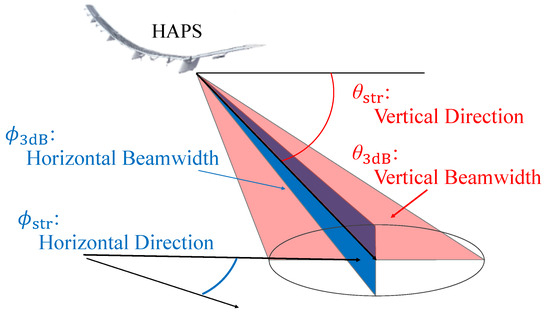
Figure 2.
Beam parameters for a cell.
Subsequently, we describe the calculations for the signal-to-noise ratio (SNR) and signal-to-interference-plus-noise ratio (SINR). The downlink (DL) received signal level for the u-th UE from the c-th cell in dB is as follows:
Here, , , and denote the BS transmission power, the BS antenna gain of the c-th cell for the u-th UE, which follows Equation (2), and the antenna gain for UE, respectively. denotes the free-space path loss in dB between the u-th UE and HAPS, which is expressed as
Here, and denote the distance between the u-th UE and HAPS, and the wavelength, respectively. In this case, we calculate N values for the u-th UE, where N denotes the number of cells in a HAPS. We define the cell to which the u-th UE is attached as the cell with the highest receiver level among the N cells. Let represent the cell index to which the u-th UE attaches. In such a case, the total interference power of the u-th UE, which is attached to the -th cell, can be expressed in dB as follows:
where stands for an activation factor, denoting the number of resource blocks (RBs) used in neighboring cells. We assume to be 0.5, suggesting that 50% of the RBs in the neighboring cells are used for interference calculations. Consequently, for the u-th UE attached to the c-th cell, the values for DL SNR and DL SINR in dB can be expressed as follows:
and
Here, denotes the noise power in a linear scale. The calculation of the noise power in dB, which is the conversion of to a dB scale, can be expressed as follows:
where B and F denote the bandwidth and the noise figure, respectively. Following the same procedure as DL, the uplink (UL) received signal level of the u-th UE in the c-th cell is as follows:
where stands for the UE transmission power. The UE attaches to the cell that has the maximum DL received power, designated as . Here, we employ coordinated multi-point (CoMP) reception for the UL, a technique widely adopted in mobile wireless communications systems, such as 4G LTE. The UL CoMP enables us to achieve diversity gain by receiving signals from UE across multiple neighboring cells, thereby enhancing the UL SNR, especially at cell borders, which extends the coverage area. In this paper, we consider UL CoMP with two cells. If the second strongest signal power from the u-th UE is denoted as , where , the UL SNR considering UL CoMP is expressed as follows:
2.2. Dynamic Area Optimization Using GA: An Overview and Challenges
The application of search methods for dynamic area optimization offers an effective way to explore better antenna parameters that improve communication quality for user distribution. In this study, we choose GA as the search method and utilize the generated solutions as our training data. The focus of this study is to optimize the horizontal beam directions exclusively, as an initial investigation, specifically for the three-cell and six-cell scenarios. Figure 3 illustrates the heatmap of the GA-optimized beam accounting for the user distribution in a three-cell scenario. The red dots are the user position, and the yellow regions indicate areas with high beam power. In GA, based on the value of the fitness function, the top individuals are preserved as elites, and the others undergo crossover and mutation to generate the next generation. In this study, we assigned each individual a horizontal beam direction for each cell and set the rate of the elites, crossover, and mutation to 5%, 80%, and 15%, respectively. The implementation of crossover and mutation is based on the literature [28]. Other GA parameters, i.e., the population size, convergence generation, and maximum generation are set to 100, 100, and 1000, respectively, to ensure sufficient exploration during the GA search process. Furthermore, based on [29], the fitness function is defined as a penalty function that combines the objective function and the amount of violation for constraint conditions. We essentially used the settings for GA that delivered good outcomes in an earlier study [23,24], where they evaluated and discussed these parameters in detail. The implementation of the GA was primarily facilitated using MATLAB’s Global Optimization Toolbox. For further details regarding the GA methodology, reference is made to MATLAB’s comprehensive documentation.

Figure 3.
SINR Heatmap based on the beams obtained by genetic algorithm (GA).
In our approach, we enforce constraints to maintain a basic level of communication quality to ensure full coverage of the service area. Specifically, we employ the constraint conditions for SNR and SINR in studies [23,24], which are defined as follows:
Here, , , and represent the first percentile thresholds of the DL SNR, DL SINR, and UL SNR for users in the area. These are calculated in Equation (7), Equation (8) and Equation (11), respectively. The DL SINR value given here is under full buffer conditions. A safety margin of 15 dB from the required SNR and SINR is included within these constraints. When evaluating these constraints, a uniform user distribution is assumed to ensure that coverage standards are met even in user-absent regions.
In defining the objective function, we utilize an indicator that factors in proportional fairness (PF) [30] across users on a per cell basis. It is represented as follows:
where B denotes the bandwidth, and denote the number of users in all areas and the number of users located in the c-th cell for u-th user, respectively. denotes the SINR for the u-th user. This objective function is designed with reference to the Nash equilibrium, assuming that each user’s throughput is maximized by PF [31].
With the settings above, the optimization problem is formulated as follows:
Here, and mean the horizontal beam directions for each cell and all possible combinations of them, respectively. The optimization based on the search algorithm efficiently obtains near-optimal parameters. However, as mentioned in Section 1, the frequent optimization by the search methods and the growing search space proportional to cells or parameters induce an increase in the computational cost of the searches, which hinders the prompt adaptation to sudden distribution changes resulting from natural disasters or major events.
3. Dynamic Area Optimization Based on an NN Considering Intercell Relationships
3.1. Dynamic Area Optimization through the Application of NN
This study introduces an area optimization approach based on a supervised learning model that is pretrained on the solutions obtained by GA to address the problem mentioned in Section 2. Due to a complicated relationship between user distribution and beam parameters in area optimization, linear regression or rule-based models cannot precisely represent the relationships. Therefore, we choose an NN model that can learn nonlinear relationships and is easy to implement.
Employing the supervised learning model enables us to utilize previous solutions as the training data. After the training process, the model no longer needs to explore solutions, which is a necessary step in the case of GA. Additionally, the computational process for prediction is simplified to matrix multiplication, greatly lowering the computational cost and enabling prompt adjustment to sudden distribution shifts.
The NN learns GA optimization results, as illustrated in Figure 4. The inputs and outputs consist of the user distribution information and the optimal horizontal beam directions generated by GA, respectively. To obtain the statistical information on user distribution within the service area, the area is partitioned uniformly into fan-shaped segments, and the user densities in the segments are utilized as the inputs for NN. The k-th input for the m-th NN model () and the inputs for the m-th model () are expressed as follows:
Here, and represent the number of users in the k-th sector and across all sectors, respectively. We have adopted fan-shaped segments to avoid overfitting caused by overly detailed inputs, enable the acquisition of necessary horizontal information for learning the horizontal beam directions, and simplify the mapping between inputs and outputs. The model employs the categorical cross-entropy loss function, which is commonly used in multiclass classification. The function can be expressed as follows:
Herein, n, , k, and K represent the data index, the total amount of data, the class index, and the number of classes, respectively. and indicate the true class for the n-th data, that is, whether it belongs to class k or not (indicated by 1 or 0), and the probability of the n-th data belonging to the k-th class. The k-th class is considered the k-th fan-shaped segment in this study. To estimate the horizontal beam direction, we utilize the angle bisector of this k-th segment. This configuration is used as the basis for training the model that estimates the horizontal beam direction.

Figure 4.
Neural network (NN) learning the solutions generated by GA.
Nevertheless, as depicted in Figure 5, interferences or uncovered areas among beams (or cells) can arise due to an incorrect cell interval when antenna parameters for the multicell configuration are output either all at once or separately for each cell. Consequently, communication capacity cannot be fully improved. The problem stems from the fact that each cell learns independently, optimizing its own beams without accounting for those of neighboring cells. This implies a need to consider the interactions among neighboring cells during the learning process to effectively improve communication capacity.
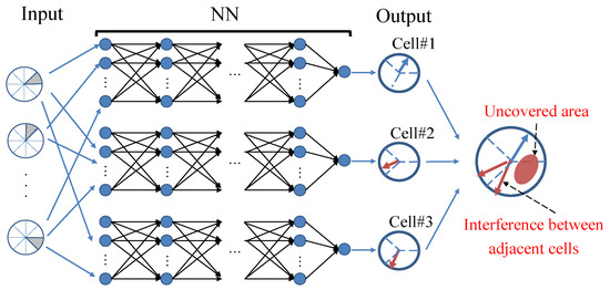
Figure 5.
Challenge encountered in area optimization using individually trained NNs.
3.2. Utilizing CC to Learn Cell Relationships
To account for the interactions among adjacent cells, we introduce Classifier Chain (CC) [32] into the NN learning process. The CC chains multiple classifiers to learn output relationships. Particularly from the second classifier onward, the estimates produced by previous classifiers are incrementally added to the input data, which effectively exploits the estimated information. This operation facilitates the consideration of relationships among outputs. The input for the m-th model () and all the beam directions predicted by the CC models () are expressed as follows:
where is the beam direction predicted by the m-th CC model. The loss function remains the same as the one used in the NN, as shown in Equation (17). This method enhances the accuracy of estimations by accounting for intercell relationships.
Figure 6 illustrates the model structure when CC is incorporated into the horizontal beam directions across three cells. Here, the inputs are the user densities mentioned earlier. The CC captures the relationship between neighboring beams by adding the solutions to the following models. As depicted in Figure 6, the output for cell #2 is predicted based on its relationship to cell #1, while the output for cell #3 is predicted based on its relationship to cell #1 and cell #2.
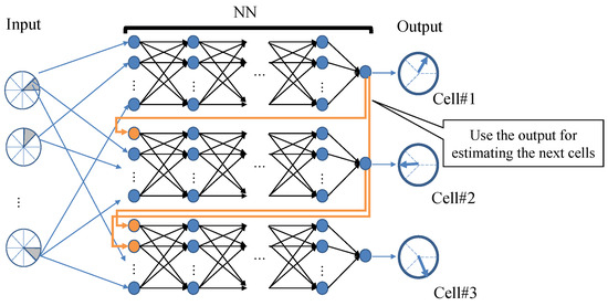
Figure 6.
Example of model configuration using CCs (cells #1, #2, and #3 in sequence).
3.3. Ensemble Approach for Objective Function Maximization
In the example depicted in Figure 6, the cells are output in an order from #1 to #3. However, the capability of the CC might fluctuate depending on the sequence of the cell output. This variation happens because the optimal prioritization for cell predictions depends on user distribution. To address this problem, we apply an ensemble approach that produces the CCs for potential sequences and chooses the solution with the highest objective function value from the obtained solutions. An example of the ensemble method for three-cell configurations is illustrated in Figure 7. When optimizing the horizontal beam direction for three cells, there could be 3! (i.e., 6) possible permutations of CCs. Among these, the solution scoring the highest objective function value is chosen. The definition of the objective function is consistent with that of GA, as indicated in Equation (13). The best sequence of all CC permutations () is expressed as follows:
where and are the beam directions predicted by the i-th order CC and the objective function by the beam directions , respectively.
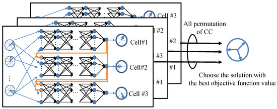
Figure 7.
Schematic of the ensemble approach (Three-cell horizontal beam directions).
3.4. Quality Control against Estimation Errors
Beam estimations produced by the learning model may not always be precise, potentially leading to a decline in communication quality. In such scenarios, maintaining a minimum level of communication quality that is independent of the model’s estimates is essential. To manage this, we utilize a process workflow as illustrated in Figure 8. From the solutions generated by the learning model, those that meet the constraints and enhance the objective function are chosen. If not, the uniform beam placement (default parameters) is deployed. The default parameters account for a uniform distribution unbiased in the population distribution, resulting in evenly placed beam directions across the area, and meet the constraints indicated in Equation (12). The solution is expressed as follows:

Figure 8.
The workflow of NN-based dynamic area optimization from input to output.
4. Evaluation
In this section, we first explain the evaluation conditions and subsequently present the evaluation of the communication performance and cost of the proposed method.
4.1. Evaluation Conditions
We evaluated the optimization of the horizontal beam direction for three- and six-cell configurations. The horizontal beamwidth, vertical beam direction, and vertical beamwidth values were set to optimal solutions under a uniform distribution. These values are 42°, 48°, and 28° for the three-cell configuration, and 28°, 36°, and 32° for the six-cell configuration, with the same values for all cells. The user distributions used in the simulation, which were modeled based on user data supplied by the Agoop Corporation [33], utilized a mobile population within a 30 km radius, configured in a mesh format, as demonstrated in Figure 9. Figure 9a,b present examples of dense and sparse areas in Japan, respectively. We assume that the estimation of the user distribution data can be realized by some methods, such as the method of analyzing the power that the BS receives or the method utilizing Minimization of Drive Tests [34]. Table 1 and Table 2 list the specifics of the beam and learning parameters, respectively. In this study, we consider a line-of-sight environment for the propagation model and entail free-space loss. Following a prior study [35], we assume the antenna gain of the user terminals to be dBi. For the DL and UL, we set the noise figures at 5 dB and 3 dB, respectively, which reflect common values for commercial terminals and BSs. A dataset of 20,000 user distributions is provided and divided into an 8:2 ratio for training and testing of the NN model. In our preliminary simulations, we determined the selectable variables for the NN, including the degree of the fan-shaped area, the number of hidden layers, and the number of nodes in each layer. We randomly tested combinations of these parameters; we selected the degree of the fan-shaped area from 2, 5, 10, 20, and 30, the number of hidden layers from 1 to 5, and the number of nodes from 16, 32, 64, 128, 256, 512, and 1024, respectively. The combination that demonstrated the highest performance with the training data was selected. As a result, the optimal parameters were determined as a 20 degree for the fan-shaped area and the NN architecture consisting of 4 hidden layers with 64 nodes each. In terms of software, all computations were executed using MATLAB version R2022a with the Deep Learning Toolbox for model training. From a hardware perspective, we utilized an AMD Ryzen Threadripper 3970X 32-Core Processor operating at 3.69 GHz with 256 GB RAM, running a 64-bit version of Windows 11 Pro OS. Graphics processing was handled by an NVIDIA GeForce RTX 3090 graphics processing unit with a 24 GB memory. The time evaluation was performed using only 1 core or without parallelization to ensure a fair evaluation.
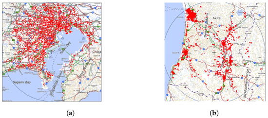
Figure 9.
Example of user distributions. (a) Dense area around Tokyo. (b) Sparse area around Akita.

Table 1.
Beam Parameters.
Table 2.
Learning Parameters.
4.2. Communication Performance
Herein, we evaluate the effectiveness of our method by comparing communication performance metrics between our proposed method and GA. Furthermore, the detailed techniques in our proposed method are compared. Specifically, we compare the NN learning cell separately (“NN”), the CC learning cell with the relationship (“NN+CC”), and the ensemble approach learning cooperatively (“NN+CC+Ensemble”). We aim to identify the significance of each technique by analyzing them separately. It should be noted that, for this comparison, the default state involves uniformly placed beams within the area.
Initially, we compare the DL SINR heatmaps generated by each method for a user distribution to visually understand how the CC and the ensemble method affect the NN. The heatmaps are illustrated in Figure 10. The black dashed arrows depict the beam directions predicted by each method. There is a notable reduction in SINR for the NN estimation, due to interference between the cells at the upper and left positions, as well as an uncovered area between the left and bottom-right cells. The addition of CC appears to solve the cell interval adjustment problems. However, the predicted beam solutions depend on the sequence of the CC. To select the best solution with the highest objective function value across all the solutions, the ensemble approach is employed. In Figure 10, the heatmap surrounded by the red box offers the highest objective function value and is chosen by the ensemble approach. The heatmap is comparable to the one generated by the GA beam solution. This indicates that, despite the variations caused by the learning sequences of the CCs, the ensemble approach identifies the suitable pattern that improves communication quality as much as the GA beam solution.
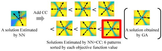
Figure 10.
SINR heatmaps based on the estimated beams for three-cell configuration (NN, NN+CC, and GA).
Subsequently, we compare constraint violation ratios, which are the distribution ratios wherein the constraints are violated among all user distributions, for each method. Incidentally, the quality control detailed in Section 3 was not applied here because it would make the ratios zero, and we would not be able to evaluate the ratios after the control. Figure 11 illustrates the constraint violation ratios in the three-cell and six-cell configurations for the NN, NN+CC, and NN+CC+Ensemble. The ratios for each method are 46.7%, 7.9%, and 0.2%, respectively, in the three-cell configuration, and 78.5%, 32.8%, and 0%, respectively, in the six-cell configuration. These results indicate that NN+CC and NN+CC+Ensemble significantly reduce the constraint violation ratios in both configurations. This improvement is largely due to the incorporation of CC, which considers the intervals between neighboring cells, and mitigates interferences and uncovered areas. Furthermore, for the ensemble approach, the decline of the constraint violation ratio is greater than NN+CC. This is because the ensemble approach has many solution candidates and can select superior solutions for the constraints from them. It should be noted that the constraint violation ratios are greater for the six-cell condition than for the three-cell condition in both NN and NN+CC scenarios, which is caused by the learning difficulty due to more complex beam relationships in a six-cell configuration.
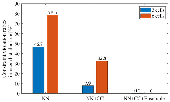
Figure 11.
Constraint violation ratios for three- and six-cell configurations (NN, NN+CC, NN+CC+Ensemble).
Figure 12 depicts the cumulative distribution functions (CDFs) of the total throughput in the three-cell and six-cell configurations when each method is applied to all the user distributions. The total throughput T is based on Shannon’s theory and defined as follows:
In both three- and six-cell conditions, the total throughput improves gradually by incorporating the CC and ensemble approach when compared with the default state. We evaluate this based on the degradation ratio, which measures how much the total throughput median of each method is degraded compared to that of GA. In the three-cell condition, the degradation ratio is 10.5% for the default state, while it reduces to 5.6%, 2.9%, and 1.1% for NN, NN+CC, and NN+CC+Ensemble, respectively. In the six-cell condition, it is 13% for the default state, whereas it reduces to 11%, 7.5%, and 0.67% for NN, NN+CC, and NN+CC+Ensemble, respectively. The CDFs achieved by NN+CC+Ensemble align well with those of GA, suggesting that accounting for neighboring cell relationships with the aid of CC refines beam intervals, thereby improving throughput. Furthermore, the incorporation of the ensemble approach helps to select the best prediction from all CC predictions with different performances for various user distributions. Incidentally, in the six-cell condition, the improvements by NN and NN+CC are smaller than those of the three-cell condition. The main reason for this observation is the high complexity of learning neighboring beam relationships by changing the configuration from three-cell to six-cell. This is almost the same as the discussion on the constraint violation ratio mentioned earlier.

Figure 12.
Cumulative distribution curves of the total throughput for the (a) three- and (b) six-cell configurations.
Figure 13 presents the CDFs of the errors between the predicted and learned beam directions, averaged for each cell. The error E is expressed as follows:
where C is the number of cells, and and are the predicted and learned beam direction of the c-th cell, respectively. The function is expressed as follows:
The error E considers the possibility of the prediction being offset by one cell. For instance, in the case of a three-cell configuration, the degrees of (0, 120, 240) could be predicted as (120, 240, 360). It should be noted that and mean and , respectively, for simplicity. The CDFs of the errors in the three-cell and six-cell configurations are depicted in Figure 13a and Figure 13b, respectively. There is an improvement in the errors for both configurations. Nevertheless, despite the similarity in the total throughput between our proposed method and GA, as shown in Figure 12, our method still predicts some beams incorrectly. For the three-cell condition (Figure 13a), the majority of errors, accounting for around 80%, are less than 10°, whereas the leftover errors range from 10° to 60°. Likewise, for the six-cell condition (Figure 13b), nearly 80% of the errors are less than 5°, whereas the leftover errors range from 5° to 30°. Two main reasons can be attributed to achieving the same total throughput as GA in our proposed method, despite the presence of errors. The one is that small errors have less impact on throughput when using large horizontal beamwidths, specifically around 40° for the three-cell condition and around 30° for the six-cell condition. The other is that depending on the user distribution, throughput remains relatively unaffected by errors in the beams in some scenarios.
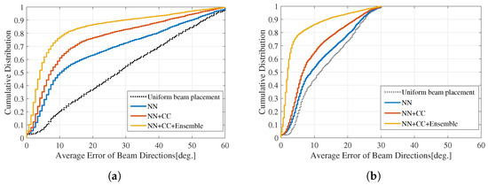
Figure 13.
Cumulative distribution curves of the errors for the beam directions, averaged for each cell. (a) Three-cell configuration. (b) Six-cell configuration.
4.3. Cost Evaluation
Here, we evaluate several factors related to calculation costs caused by our proposed method, including the number of models required for the ensemble approach, amount of training data, and total computation time. First, our ensemble approach involves all permutations of the CC models. However, as the number of cells increases, the number of possible model permutations grows exponentially, increasing the computational cost. Therefore, we evaluate the number of models necessary for the ensemble. Second, because the amount of training data directly impacts the training time and costs, we evaluate the amount of training data required to accomplish throughput performance comparable to that of GA. Finally, we compare the total time required for optimizing each user distribution, which includes both the training and prediction times, to that of GA to determine the efficiency of the proposed method.
Figure 14 illustrates the relationship between the number of CC models employed in the ensemble approach and the median of total throughput for the six-cell configuration. The models were randomly selected from the permutations of the six cells for reducing the number of models, and the average of the total throughput medians was calculated. As a side note, this evaluation was not carried out for the three-cell configuration owing to the small number of permutations; thus, no reduction was necessary. Conversely, the six-cell configuration required reduction owing to the large number of permutations. As depicted in Figure 14, the median of the total throughput decreases with the reduction in the number of models. In particular, when the number of models reduces to 100 or less, the median of the total throughput falls drastically. Specifically, it is 13.2% for the default state, whereas it is 0.38%, 0.84%, 1.11%, 2.69%, and 8.10% when employing 720, 200, 100, 10, and 1 models, respectively. This implies that even with a certain degree of model reduction, the degradation ratios remain small. This can be attributed to the similar values obtained from permutations of CC estimations. The CC models trained in similar sequences generate similar outputs. The result suggests that, by allowing a certain level of degradation, the number of models can be pruned. For example, accepting a degradation tolerance of roughly 1.1% allows a reduction in the number of models by 1/7 (roughly 100 out of 720).
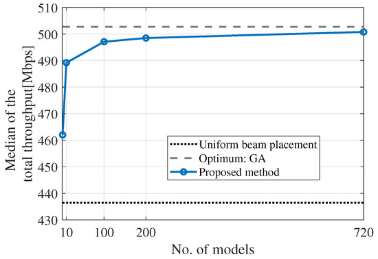
Figure 14.
Relationship between the total throughput median and the number of extracted models for the ensemble approach.
Figure 15 illustrates the relationship between the amount of training data and the total throughput median for the six-cell configuration. To evaluate the required amount of training data for this problem, the amount of training data varying from 4000 to 36,000 is exclusively utilized for this evaluation. This figure includes results from NN, NN+CC, and NN+CC+Ensemble with 720 models, as well as NN+CC+Ensemble with 100 models selected randomly. It can be observed that the total throughput medians for NN+CC+Ensemble with 720 and 100 models converge from 16,000 data points, reaching 498 and 496 Mbps, respectively. Therefore, 16,000 data points are considered sufficient for training in this study. This convergence can be attributed to the increased generalizability of the models as the patterns in the training data expand, thereby improving adaptability to the test data. Conversely, it can also be observed that increasing the amount of training data does not significantly impact the performance of the NN. This is primarily attributed to insufficient information for learning. The information from adjacent cells is essential, and the integration of this information into the input through the NN+CC enhances performance.
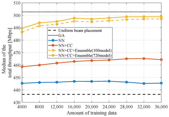
Figure 15.
Relationship between the total throughput median and the training data amount.
Figure 16 shows the relationship between the number of optimized distributions and the total time required for optimizing each user distribution for GA and the proposed method with an ensemble of 720 and 100 models. Table 3 lists the average time required for training and prediction for each method. GA was executed using only 1 core or without parallelization, whereas the ensemble model training was executed sequentially with one model each to ensure a fair evaluation. We employ 16,000 distributions for training and 1 distribution for each prediction. It should be noted that the proposed method requires training time, which GA does not; therefore, the training time is added at the point of 0 distribution in Figure 16. From this figure, it can be observed that at first, the proposed method falls behind the GA due to the training time; however, it gradually fills the gap and overtakes GA. Specifically, the times for the 720 and 100 models are shorter from approximately 170 and 25 distribution points, respectively, than those for the GA. This is attributed to the prediction speed of the proposed methods. The prediction times for NN+CC+Ensemble with 720 and 100 models in Table 3 are approximately 14 and 100 times faster, respectively, than those for GA. Additionally, from the perspective of the training time, it is evident that the times for NN+CC+Ensemble with 720 and 100 models in Table 3 are not long. Specifically, they are 30 and 4 h, respectively. Considering that the training can be executed in advance and the models do not have to be updated frequently, these values are within practical limits. It should be noted that the extended time required for NN+CC+Ensemble, compared with those for NN and NN+CC, is mainly due to the number of models. Specifically, in scenarios with 720 and 100 models, the prediction times necessary for NN+CC+Ensemble are approximately 780 and 110 times longer than those required for NN+CC, respectively. Although reducing the number of models in the ensemble approach may slightly degrade the throughput, it can significantly enhance the optimization speed.

Figure 16.
Relationship between the total time taken for optimizing each user distribution and the number of optimized distributions.
Table 3.
Time for training and prediction for each method.
5. Conclusions and Future Work
In this study, we have presented an NN-based dynamic area optimization method that matches the performance of a GA. The method is easy to implement and allows for instant adaptation of the system in response to shifts in the user distribution. With the utilization of NN for dynamic area optimization, problems such as interference or uncovered areas between cells may arise due to incorrect beam intervals, which prevent sufficient communication capacity improvement. To account for adjacent cell relationships during training, we integrate a CC into the NN. Nevertheless, a CC might face learning order challenges depending on the user distribution, which causes performance fluctuations. Thus, our proposed method employs an ensemble approach to integrate multiple CC variations and choose the pattern best suited for the objective function. The simulation results demonstrate notable improvements in the optimization of horizontal beam directions for both three- and six-cell configurations. In addition, the number of models used in the ensemble approach can be scaled down by allowing a certain level of performance reduction. Further, the time efficiency of the proposed method exceeds that of GA because the training time is relatively short and the prediction speed is high.
This study’s evaluation is solely based on the results learned and predicted from the data we prepared. It is important to highlight that there may still be challenges when it comes to real-world applications. For instance, if the dataset changes, the amount of learning data necessary for accurate results could increase, and performance may vary. To tackle this, we could consider gathering broader and more diverse learning data to improve the model’s robustness. Recent advancements like transfer learning and federated learning could also be beneficial. Transfer learning can adjust the model to specific areas, while federated learning can increase flexibility by merging models trained in different areas. These methods might enhance our approach.
Author Contributions
Conceptualization, W.T.; methodology, W.T. and Y.S.; validation, W.T. and Y.S. and K.H.; formal analysis, W.T. and Y.S.; writing—original draft preparation, W.T. and Y.S.; writing—review and editing, W.T., Y.S., K.H. and T.O. All authors have read and agreed to the published version of the manuscript.
Funding
This work was supported in part by the National Institute of Information and Communications Technology (NICT) in Japan under Grant Number JPJ012368C05701.
Data Availability Statement
The datasets presented in this article are not available because the data was obtained from user devices affiliated with our company and the public disclosure of this information is restricted.
Conflicts of Interest
Wataru Takabatake, Yohei Shibata, Kenji Hoshino are currently employed at the SoftBank Corp. Technology Research Laboratory. The remaining author declares that the research was conducted in the absence of any commercial or financial relationships that could be construed as a potential conflict of interest. The funders had no role in the design of the study; in the collection, analyses, or interpretation of data; in the writing of the manuscript; or in the decision to publish the results.
Abbreviations
The following abbreviations are used in this manuscript:
| HAPSs | High-altitude platform stations |
| GA | Genetic algorithm |
| NN | Neural network |
| CC | Classifier chain |
| CDF | Cumulative distribution function |
| 4G LTE | Fourth-generation long-term evolution |
| 5G NR | Fifth-generation new radio |
| UAVs | Unmanned aerial vehicles |
| RTT | Round trip time |
| BSs | Base stations |
| RL | Reinforcement learning |
| OFDMA | Orthogonal frequency-division multiple access |
| DRL | Deep reinforcement learning |
| MCS | Modulation and coding scheme |
| CSI | Channel state information |
| SNR | Signal-to-noise ratio |
| SINR | Signal-to-interference-plus-noise ratio |
| DL | Downlink |
| RBs | Resource blocks |
| UL | Uplink |
| CoMP | Coordinated multi-point |
| PF | Proportional fairness |
References
- Karapantazis, S.; Pavlidou, F. Broadband communications via high-altitude platforms: A survey. IEEE Commun. Surv. Tutor. 2005, 7, 2–31. [Google Scholar] [CrossRef]
- Nagate, A.; Ota, Y.; Hoshino, K. HAPS radio repeater system using the same system as terrestrial mobile communications system. IEICE Soc. Conf. 2018, 5, 37. (In Japanese) [Google Scholar]
- Study on Using Satellite Access in 5G; 3GPP Document TR22.822 V16.0.0. Available online: https://portal.3gpp.org/desktopmodules/Specifications/SpecificationDetails.aspx?specificationId=3372 (accessed on 8 September 2024).
- Qian, S.; Zhang, S.; Zhou, W. Traffic-based dynamic beam coverage adjustment in satellite mobile communication. In Proceedings of the Sixth International Conference on Wireless Communications and Signal Processing (WCSP), Hefei, China, 23–25 October 2014; pp. 1–6. [Google Scholar]
- Tang, J.; Bian, D.; Li, G.; Hu, J.; Cheng, J. Optimization method of dynamic beam position for LEO beam-hopping satellite communication systems. IEEE Access 2021, 9, 142–149. [Google Scholar] [CrossRef]
- Lin, Z.; Lin, M.; Wang, J.-B.; de Cola, T.; Wang, J. Joint beamforming and power allocation for satellite-terrestrial integrated networks with nonorthogonal multiple access. IEEE J. Sel. Areas Commun. 2019, 13, 657–670. [Google Scholar]
- Lin, Z.; Lin, M.; De Cola, T.; Wang, J.B.; Zhu, W.P.; Cheng, J. Supporting IoT with rate-splitting multiple access in satellite and aerial-integrated networks. IEEE Internet Things J. 2021, 8, 11123–11134. [Google Scholar] [CrossRef]
- Lin, Z.; Lin, M.; Champagne, B.; Zhu, W.-P.; Al-Dhahir, N. Secure and Energy Efficient Transmission for RSMA-Based Cognitive Satellite-Terrestrial Networks. IEEE Wirel. Commun. Lett. 2021, 10, 251–255. [Google Scholar] [CrossRef]
- Dirani, M.; Altman, Z. A cooperative reinforcement learning approach for intercell interference coordination in OFDMA cellular networks. In Proceedings of the 8th International Symposium on Modeling and Optimization in Mobile, Ad Hoc, and Wireless Networks, Avignon, France, 31 May–4 June 2010; pp. 170–176. [Google Scholar]
- Bennis, M.; Niyato, D. A Q-learning based approach to interference avoidance in self-organized femtocell networks. In Proceedings of the 2010 IEEE Globecom Workshops, Miami, FL, USA, 6–10 December 2010; pp. 706–710. [Google Scholar]
- Shafin, R.; Chen, H.; Nam, Y.H.; Hur, S.; Park, J.; Zhang, J.; Liu, L. Self-tuning sectorization: Deep reinforcement learning meets broadcast beam optimization. IEEE Trans. Wirel. Commun. 2020, 19, 4038–4053. [Google Scholar] [CrossRef]
- Balevi, E.; Andrews, J.G. A novel deep reinforcement learning algorithm for online antenna tuning. In Proceedings of the 2019 IEEE Global Communications Conference (GLOBECOM), Waikoloa, HI, USA, 9–13 December 2019; pp. 1–6. [Google Scholar]
- Khoshkbari, H.; Pourahmadi, V.; Sheikhzadeh, H. Bayesian reinforcement learning for link-level throughput maximization. IEEE Commun. Lett. 2020, 24, 1738–1741. [Google Scholar] [CrossRef]
- Jamshidiha, S.; Pourahmadi, V.; Mohammadi, A.; Bennis, M. Link-level throughput maximization using deep reinforcement learning. IEEE Netw. Lett. 2020, 2, 101–105. [Google Scholar] [CrossRef]
- Sharifi, S.; Khoshkbari, H.; Kaddoum, G.; Akhrif, O. Deep reinforcement learning approach for haps user scheduling in massive mimo communications. IEEE Open J. Commun. Soc. 2024, 5, 1–14. [Google Scholar] [CrossRef]
- Jo, S.; Yang, W.; Choi, H.K.; Noh, E.; Jo, H.-S.; Park, J. Deep Q-learning-based transmission power control of a high altitude platform station with spectrum sharing. Sensors 2022, 22, 1630. [Google Scholar] [CrossRef] [PubMed]
- Eckhardt, H.; Klein, S.; Gruber, M. Vertical antenna tilt optimization for LTE base stations. In Proceedings of the 2011 IEEE 73rd Vehicular Technology Conference (VTC Spring), Budapest, Hungary, 15–18 May 2011; pp. 1–5. [Google Scholar]
- Peyvandi, H.; Imran, A.; Imran, M.A.; Tafazolli, R. On pareto-koopmans efficiency for performance-driven optimisation in self-organising networks. In Proceedings of the IET Intelligent Signal Processing Conference 2013 (ISP 2013), London, UK, 2–3 December 2013; pp. 1–6. [Google Scholar]
- Aliu, O.G.; Mehta, M.; Imran, M.A.; Karandikar, A.; Evans, B. A new cellular-automata-based fractional frequency reuse scheme. IEEE Trans. Veh. Technol. 2015, 64, 1535–1547. [Google Scholar] [CrossRef]
- Ho, L.T.W.; Ashraf, I.; Claussen, H. Evolving femtocell coverage optimization algorithms using genetic programming. In Proceedings of the 2009 IEEE 20th International Symposium on Personal, Indoor and Mobile Radio Communications, London, UK, 13–16 September 2009; pp. 2132–2136. [Google Scholar]
- Mohjazi, L.S.; Al-Qutayri, M.A.; Barada, H.R.; Poon, K.F.; Shubair, R.M. Self-optimization of pilot power in enterprise femtocells using multi objective heuristic. J. Comput. Netw. Commun. 2012, 2012, 1535–1547. [Google Scholar] [CrossRef][Green Version]
- Klaine, P.V.; Imran, M.A.; Onireti, O.; Souza, R.D. A survey of machine learning techniques applied to self-organizing cellular networks. IEEE Commun. Surv. Tutor. 2017, 19, 2392–2431. [Google Scholar] [CrossRef]
- Shibata, Y.; Kanazawa, N.; Konishi, M.; Hoshino, K.; Ohta, Y.; Nagate, A. System design of gigabit HAPS mobile communications. IEEE Access 2020, 8, 157995–158007. [Google Scholar] [CrossRef]
- Shibata, Y.; Takabatake, W.; Hoshino, K.; Nagate, A.; Ohtsuki, T. Two-step dynamic cell optimization algorithm for HAPS mobile communications. IEEE Access 2022, 10, 68085–68098. [Google Scholar] [CrossRef]
- Takabatake, W.; Shibata, Y.; Hoshino, K. Neural-Network-based Dynamic Area Optimization Algorithm for High-Altitude Platform Station. In Proceedings of the 2023 IEEE 98th Vehicular Technology Conference (VTC2023-Fall), Hong Kong, China, 10–13 October 2023; pp. 1–6. [Google Scholar]
- Hoshino, K.; Sudo, S.; Ohta, Y. A Study on Antenna Beamforming Method Considering Movement of Solar Plane in HAPS System. In Proceedings of the 2019 IEEE 90th Vehicular Technology Conference (VTC2019-Fall), Honolulu, HI, USA, 22–25 September 2019; pp. 1–5. [Google Scholar]
- Minimum Performance Characteristics and Operational Conditions for High Altitude Platform Stations Providing IMT-2000 in the Bands 1885–1980 MHz, 2010–2025 MHz and 2110–2170 MHz in Regions 1 and 3 and 1885–1980 MHz and 2110–2160 MHz in Region 2 Document ITU-R M.1456; International Telecommunications Union: Geneva, Switzerland, 2000.
- Deep, K.; Singh, K.P.; Kansal, M.L.; Mohan, C. A real coded genetic algorithm for solving integer and mixed integer optimization problems. Appl. Math. Comput. 2009, 212, 505–518. [Google Scholar] [CrossRef]
- Deb, K. An efficient constraint handling method for genetic algorithms. Comput. Methods Appl. Mech. Eng. 2000, 186, 311–338. [Google Scholar] [CrossRef]
- Liu, Y.-F.; Dai, Y.-H.; Luo, Z.-Q. Coordinated beamforming for MISO interference channel: Complexity analysis and efficient algorithms. IEEE Trans. Signal Process. 2010, 59, 1142–1157. [Google Scholar] [CrossRef]
- Yamamoto, K. Application of game theory to wireless communications. J. IEICE 2012, 95, 1089–1093. (In Japanese) [Google Scholar]
- Read, J.; Pfahringer, B.; Holmes, G.; Frank, E. Classifier chains for multi-label classification. Mach. Learn. 2011, 85, 333–359. [Google Scholar] [CrossRef]
- Dynamic Population Data. Agoop Corporation. Available online: https://www.agoop.co.jp/service/dynamic-population-data/ (accessed on 29 May 2023).
- Johansson, J.; Hapsari, W.A.; Kelley, S.; Bodog, G. Minimization of drive tests in 3GPP release 11. IEEE Commun. Mag. 2012, 50, 36–43. [Google Scholar] [CrossRef]
- Grace, D.; Mihael, M. Broadband Communications via High-Altitude Platforms; John Wiley & Sons: Hoboken, NJ, USA, 2011. [Google Scholar]


Disclaimer/Publisher’s Note: The statements, opinions and data contained in all publications are solely those of the individual author(s) and contributor(s) and not of MDPI and/or the editor(s). MDPI and/or the editor(s) disclaim responsibility for any injury to people or property resulting from any ideas, methods, instructions or products referred to in the content. |
© 2024 by the authors. Licensee MDPI, Basel, Switzerland. This article is an open access article distributed under the terms and conditions of the Creative Commons Attribution (CC BY) license (https://creativecommons.org/licenses/by/4.0/).