Optimal Referral Reward Considering Customer’s Budget Constraint

Abstract

Everyone likes Porsche but few can afford it. Budget constraints always play a critical role in a customer’s decision-making. The literature disproportionally focuses on how firms can induce customer valuations toward the product, but does not address how to assess the influence of budget constraints. We study these questions in the context of a referral reward program (RRP). RRP is a prominent marketing strategy that utilizes recommendations passed from existing customers to their friends and effectively stimulates word of mouth (WoM). We build a stylized game-theoretical model with a nested Stackelberg game involving three players: a firm, an existing customer, and a potential customer who is a friend of the existing customer. The budget is the friend’s private information. We show that RRPs might be optimal when the friend has either a low or a high valuation, but they work differently in each situation because of the budget. Furthermore, there are two budget thresholds, a fixed one and a variable one, which limit a firm’s ability to use rewards.

1. Introduction

Everyone likes Porsche automobiles but few can afford to purchase one. Budget constraints exist among customers and play a critical role in their decision-making. An extreme Apple enthusiast might sell his or her kidney to purchase Apple products, and textbook publishers have been fighting illegal online secondhand markets and piracy websites for several years. Budget is defined as payment capacity and is independent of the customer’s product valuations [1]. In recent years, a growing number of electric commerce websites have started to provide financial support to customers with budget constraints (e.g., installment payment programs). However, the literature disproportionally focuses on how firms can induce customer valuations toward the product, but does not address how to assess the influence of budget constraints.

We study these questions in the context of a referral reward program (RRP), a prominent marketing strategy that utilizes recommendations passed from existing customers to their friends [2]. RRPs are prevalent in a wide range of industries and can be implemented through various approaches. A simple Google search of “referral reward program” returns more than three million results that cover topics such as retail stores, financing, mobile and Internet services, and electronic products. In this paper, we examine whether RRPs still work when customers have budget constraints, and determine how firms can manage situations in which RRPs do not work.

The pioneer study suggests that, when a customer’s delight threshold is at a medium level, the higher the referral rewards are, the higher the price should be [2]. However, in our study, we consider that the friends might not be able to afford a high price because of budget constraints. Therefore, the RRPs are under the risk of customers choosing to abort the program because of limited budgets rather than low valuations. We build a stylized game-theoretical model with a nested Stackelberg game involving three players: a firm, an existing customer, and a potential customer who is a friend of the existing customer. By applying backward induction in solving this nested game, we show how customers’ valuations and budget constraints could affect the design of RRPs. Benchmarked by a baseline model, we investigate the relationship between two strategies: firm financing and RRP. Firm financing refers to a strategy by which the firm allows a monetary discount the customer must pay at the moment he gets the product.

We report a line of findings by solving closed-form solutions of our analytical models. First, when the friend’s initial valuation is at a medium level, RRPs are optimal only when the friend is likely to have low budget pressure. Second, although RRPs might be optimal when the customer has either a low or a high valuation, they work differently in each situation. Third, there are two budget thresholds—a fixed one and a variable one that limit a firm’s ability to use rewards. Fourth, RRPs and firm financing, although targeting different aspects of a customer’s decision-making, can be perfectly substitutable for each other, rendering it unnecessary for firms to apply both simultaneously.

The remainder of this paper is organized as follows. First, we describe the literature on RRPs and budget constraints. Second, we introduce the proposed analytical model and discuss the results. Third, we extend the original RRP model to examine how a firm’s financing strategy can affect RRPs. Finally, we discuss the implications and limitations of our study.

2. Literature Review

There are two research streams related to our research: RRPs and budget constraints. We briefly discuss each of them in this section.

2.1. Referral Reward Programs

As effective tools to stimulate word of mouth (WoM), RRPs are proven to be profitable in marketing campaigns [2]. Various combinations of RRPs and low prices are characterized, based on the assumption that customers make a recommendation when they are delighted with a product [2].The early literature on RRPs focuses on various aspects including reward types [3,4,5,6], brand strength [7], and tie strength [4,7]. Monopolists tend to offer cash awards, whereas duopolistic firms could benefit more from offering future discounts to existing customers [3]. There are two payment functions, a linear payment function and a threshold payment function, in RRPs and anyone of them can dominate the other one under different situations [8]. Current topics in RRP studies entail customer value [9,10]. Customer lifetime value (CLV) stresses the importance of customers who can bring firms additional customers through referrals [11]. However, RRPs have controversial defects. For instance, the material rewards of RRPs add material motivation to pure friendships, and subsequently damage the receiver’s perception of the friend’s sincerity [12]. Reward types such as physical or cash rewards can exert an influence the receiver’s perception of referral motives, and thus affect the profitability of RRPs [6].

Thus far, although most RRP research is generated from empirical results, few insights are obtained through analytical models [5,13,14]. Under the assumption that customers make referrals by combining their knowledge of and familiarity with their friends’ product preferences, the firms should give out higher rewards if the customers have greater concern about their friends’ outcomes with the product they recommend [13]. The mechanisms of group buying and RRPs are both popular marketing strategies which stimulate WoM, and anyone of them can dominate the other one under different situations [14]. Meanwhile, the conditions when the firms should reward the customer only, the friend only, or reward both are investigated in an analytical model [5].

Our study considers both pricing and rewarding, and models a framework entailing a three-player market: a firm, an existing customer, and a friend [14]. Different from the previous studies which model a customer’s delight with a product as the motivating force behind a referral [2], our study assumes that referral rewards induce a customer’s referral behavior [13] and that a customer’s referral depends on both the referral award and the likelihood of the referral’s success.

2.2. Budget Constraints

The novelty of our study is that it incorporates the friend’s budget constraints into RRPs. Prior studies have focused on the friend’s valuations [2,13,14] while disregarding budget constraints.

In micro-economics, the budget is defined as the payment capability of a consumer. However, budgets are influenced by several factors such as time and income. The most significant application of budget in micro-economics is the theory of consumers, which posits that consumers purchase certain groups of products according to maximum utility within their budget. The budget constraint can be expressed as $p_1{x}_1+p_2{x}_2+\dots +p_N{x}_N\le m$, where $m$ is the budget affected by factors such as time and income; $p_N$ denotes the price of product $N$; and $x_N$ represents the number of product $N$. Therefore, the budget is a constant value in the theory of consumers. Consumers usually adopt value priority hypotheses in budget planning, especially when purchasing goods such as durables [15]. In value priority hypotheses, the budget is considered to be a constant value and the budget constraint is expressed as $p_1{g}_1+ p_2{g}_2+\dots +p_N{g}_N+y\le B$, where $B$ is a consumer’s budget, $p_N$ denotes the price of product $N$, $g_N=1\text{ or }0$ represents whether or not the consumer purchases product $N$, and $y$ is the summary of the consumer’s allocation for other goods.

There is another definition of budget different from ours. Budget is defined as the maximum a consumer plans to pay for a product, thus possibly varying with the consumer’s valuation of the product [16]. In contrast, our study defines budget as the consumer’s payment capacity, which is affected by time and income and is independent of the product valuation—the same definition as is used in the theory of consumers and value priority hypotheses [15]. There are several situations where a customer has budget constraints, especially when customers purchase durable goods such as household appliances, cars or apartments. A customer holding 30,000 dollars cannot purchase a car priced 50,000 dollars. This is a situation where the budget limits a customer’s purchase decision. The budget is the current cash state of a customer, and does not have any relationship with the product. Capacity constraint problems also occur in related research disciplines such as the budget constraint in auction literature [17] and the inventory or capital constraint in operation management.

A customer’s budget is affected by time and income, which are independent of the product valuation, follow a Bernoulli distribution (e.g., the probability of a high income is $q$, whereas the probability of a low income is $1-q$) [1]. Therefore, our study assumes that budget constraints are independent from customer valuations, and characterizes them with a Bernoulli distribution.

3. The Model and Result

We develop a nested Stackelberg game to capture the sequence of actions among three players: a firm, a customer (denoted by $\text{S}$, the information sender), and a friend (denoted by $\text{R}$, the information receiver). There are five stages for completing a RRP from Time 0 to 4. We depict the entire sequence in Figure 1. At Time 0, the firm faces Customer $\text{S}$, who has already purchased the product, and Friend $\text{R}$, who is a potential customer. At Time 1, the firm updates the price $p$ for existing customers, offering the referral reward $B$. At Time 2, Customer S chooses the increased product value $I$ for Friend R through the referral program in an effort to obtain the referral reward B (Customer S does not recommend the product if $I\le 0$). At Time 3, on the condition that Customer S opts to refer the product, Friend R decides whether to purchase it according to his or her valuation $v$ and budget $c$. Finally, at Time 4, if Friend R pays for the referred product, then Customer S receives the referral reward $B$ that the firm promised. Next, we proceed backward through the sequence to solve optimal decisions.

Figure 1. Sequence of actions.

Figure 1. Sequence of actions.

3.1. Friend R’s Problem

Friend R purchases the product when two conditions are satisfied simultaneously: First, Friend R incurs a non-negative surplus by purchasing the product (the surplus constraint). Second, in that moment, Friend R can afford the product (i.e., the price is not greater than Friend R’s budget, the budget constraint). The friend’s initial valuation of the product is denoted as $v$. Friend R’s surplus from purchasing the product (denoted by $u_R$) is then given by $u_R=v+I-p$ [14]. Thus, the surplus constraint is

$$v+I-p\ge 0$$

(1)

The budget constraint is

$$p\le c$$

(2)

Combining both constraints indicates that $p\le \min \left[c, v+I\right]$ is required for a successful referral. However, Friend R’s budget information $c$ is private. This information structure adds two layers of complexity for the firm in designing RRPs: the firm must provide sufficient incentive for Customer S to induce a larger $I$; nevertheless, the firm must remain careful about pricing, because both Friend R and Customer S are basing their decisions on the market price.

3.2. Customer S’s Problem

In our model setup, Customer S serves as a sales agent in disseminating the product information to Friend R. Unable to observe Friend R’s budget information, Customer S instead uses a Bernoulli distribution to estimate it. We assume that Customer S believes that Friend R has a budget of $H$ with the probability $q$ ($q\in \left[0,1\right]$) and a budget of $L$ ($L<H$) with the probability $1-q$ [1]. Observing the market price $p$, Customer S forms his or her own belief regarding whether Friend R will purchase the product. Denote Friend R’s action as the binary variable δ and as δ$=1$($=0$) when he or she chooses (not) to adopt. Then, the estimation of $Pr\left(\mathsf{\delta }=1\right)$ by Customer S is given by

$$Pr\left(\mathsf{\delta }=1\right)=Pr\left(p\le c\right)·\chi$$

(3)

in which

$$Pr\left(p\le c\right)=\{\begin{array}{c} 0, p\ge H\\ q, p\in \left[L,H\right)\\ 1, p<L\end{array}, \chi =\{\begin{array}{c}0, p\le v+I\\ 1, p>v+I\end{array}$$

(4)

where $\chi$ is an indicator of whether Equation (1) holds.

Given the estimation in Equation (3), a risk-neutral customer’s expected surplus of the referral (denoted by $u_S$) can be computed by $E(u_S)=Pr\left(\mathsf{\delta }=1\right)·B-\mathsf{\beta }I$, where $B$ denotes the referral reward from the firm and $\mathsf{\beta }I$ denotes the cost associated with the efforts of Customer S to increase the product value $I$ for Friend R. We consider $\mathsf{\beta }\in \left[0,1\right]$ to focus on a reasonable range of efficiency in the communication between Customer S and Friend R [14]. The problem for Customer S, therefore, is to find the optimal $I$ to maximize $E(u_S)$.

$$\underset{I}{\max }E(u_S)=Pr\left(p\le c\right)·\chi B-\mathsf{\beta }I,$$

(5)

$$\text{s.t.} Pr\left(p\le c\right)=\{\begin{array}{c} 0, p\ge H\\ q, p\in \left[L,H\right)\\ 1, p<L\end{array}, \chi =\{\begin{array}{c}0, p\le v+I\\ 1, p>v+I\end{array}, \text{and} I\ge 0.$$

(6)

3.3. The Firm’s Problem

The firm sets the price $p$ and referral reward $B$ to maximize the expected value of its profit (denoted by $\mathsf{\pi }$). Here, we assume that the firm is risk-neutral. The expected profit is $E\left(\mathsf{\pi }\right)=Pr(\mathsf{\delta }=1|I^{*}\left(p,B\right))·\left(p-B\right)$ because the firm can expect the customer’s decision on $I$, which can be solved as a function of $p$ and $B$ from Equation (5). The firm’s problem is then given by

$$\underset{p,B}{max}E\left(\mathsf{\pi }\right)=Pr(\mathsf{\delta }=1|I^{*}\left(p,B\right))\left(p-B\right)$$

(7)

$$\text{s.t.} p\ge 0, B\ge 0$$

(8)

3.4. Analysis and Results

For our analysis, we divide our discussion into three cases by locating Friend R’s initial valuation in different regions of the budget parameters: a low valuation (i.e., $v<L$), a medium valuation (i.e., $L\le v<H$), and a high valuation (i.e., $v\ge H$). We start with Lemma 1 when Friend R has a medium valuation (proofs are shown in the appendix).

Lemma 1. 

The optimal reward/price strategy is among the three candidate strategies shown in Table 1 when Friend R’s initial valuation is at the medium level ($L\le v<H$).

Table 1. Candidate strategies when $L\le v<H$.

Candidates	Price	Reward	Expected Profit
Candidate1	$L$	$0$	$L$
Candidate2	$v$	$0$	$qv$
Candidate3	$H$	$\frac{\mathsf{\beta }}{q}\left(H-v\right)$	$qH-\mathsf{\beta }\left(H-v\right)$

Table 1. Candidate strategies when $L\le v<H$.

Candidates	Price	Reward	Expected Profit
Candidate1	$L$	$0$	$L$
Candidate2	$v$	$0$	$qv$
Candidate3	$H$	$\frac{\mathsf{\beta }}{q}\left(H-v\right)$	$qH-\mathsf{\beta }\left(H-v\right)$

Lemma 1 suggests that there are multiple candidate strategies for the firm when Friend R has a medium valuation. First, the firm can simply set the price to a low level of budget $L$, which secures the firm a profit of $L$ because any budget constraint is redundant when the price is $L$. In the other two cases, the firm risks its profit by selecting either a non-reward strategy under $p=v$ or a with-reward strategy under $p=H$. The reward works only for Candidate 3, for whom the firm sets a reward to induce Customer S to persuade Friend R to purchase the product.

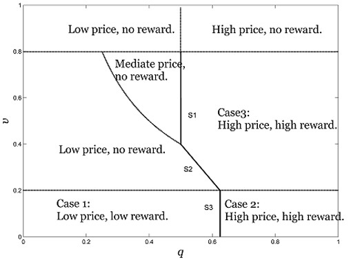
We continue to compare the profits of the three candidate strategies and derive optimality for the entire parameter space. Proposition 1 provides the results, as shown in Figure 2.

Proposition 1. 

For a medium level of initial valuation $v$ (i.e., $L\le v<H$), when $q>max\left(\mathsf{\beta },\frac{L+\mathsf{\beta }\left(H-v\right)}{H}\right),$ the firm should set a high price $H$ with reward $\frac{\mathsf{\beta }}{q}\left(H-v\right)$; when $q\le \min \left(\frac{L+\mathsf{\beta }\left(H-v\right)}{H}, \frac{L}{v}\right)$, the firm should set a low price $L$ without any referral rewards. In all other cases, the firm should set a medium price $v$ without any referral rewards.

Figure 2. Optimal strategies for the firm ($H=0.8$, $L=0.2$ and $\mathsf{\beta }=0.5$).

Figure 2. Optimal strategies for the firm ($H=0.8$, $L=0.2$ and $\mathsf{\beta }=0.5$).

As shown in Proposition 1, for an initial valuation at a medium level, Friend R’s budget affects the firm’s optimal strategies in two ways. When $q$ is small, Friend R is likely to have a small budget, inducing the firm to choose a safe price at $L$. In contrast, when $q$ is relatively large, the firm opts to choose a high price at the upper limit of Friend R’s budget, along with offering a referral reward to Customer S. The literature indicates that, when Friend R’s product valuation is not extremely high, RRPs are always profitable [14]. However, in our study, we incorporate the new dimension of budget constraints and show that the optimality of the referral strategy requires that Friend R must have not only a medium valuation, but also a large budget.

Proposition 1 suggests that boundaries for optimal strategies are sensitive to both valuations and budget constraints. When the valuation is relatively low (i.e., $L\le v<\frac{L}{\mathsf{\beta }}$), the budget threshold varies with Friend R’s valuation $v$ (as shown by curve S2 in Figure 2).

Similar to Lemma 1 and Proposition 1, we solve the firm’s optimal strategy by following Proposition 2 when $v$ is at a low level (i.e., $v<L$) or a high level (i.e., $v\ge H$).

Proposition 2. 

The firm’s optimal strategies occur when Friend R’s valuation is either low or high (Table 2).

Table 2. Firm’s optimal strategies when $v<L$ or $v\ge H$.

Conditions		Optimal Price and Reward
$v<L$	$q\le \mathsf{\beta }+\left(1-\mathsf{\beta }\right)\frac{L}{H}$	$p^{*}=L$, $B^{*}=\mathsf{\beta }\left(L-v\right)$;
	$q>\mathsf{\beta }+\left(1-\mathsf{\beta }\right)\frac{L}{H}$	$p^{*}=H$,$B^{*}=\frac{\mathsf{\beta }}{q}\left(H-v\right)$;
$v\ge H$	$q\le \frac{L}{H}$	$p^{*}=L$,$B^{*}=0$;
	$q>\frac{L}{H}$	$p^{*}=H$, $B^{*}=0$.

Table 2. Firm’s optimal strategies when $v<L$ or $v\ge H$.

Conditions		Optimal Price and Reward
$v<L$	$q\le \mathsf{\beta }+\left(1-\mathsf{\beta }\right)\frac{L}{H}$	$p^{*}=L$, $B^{*}=\mathsf{\beta }\left(L-v\right)$;
	$q>\mathsf{\beta }+\left(1-\mathsf{\beta }\right)\frac{L}{H}$	$p^{*}=H$,$B^{*}=\frac{\mathsf{\beta }}{q}\left(H-v\right)$;
$v\ge H$	$q\le \frac{L}{H}$	$p^{*}=L$,$B^{*}=0$;
	$q>\frac{L}{H}$	$p^{*}=H$, $B^{*}=0$.

First, when Friend R has limited knowledge about or a limited valuation of the product (i.e., $v<L$), it is optimal for the firm to use a RRP; however, the approach of this RRP differs from that of the RRP in Proposition 1. The optimal strategy is then divided into another two subcases on the basis of Friend R’s budget: If Friend R’s budget is likely to be high (i.e., $q>\mathsf{\beta }+\left(1-\mathsf{\beta }\right)\frac{L}{H}$), then the firm should set a high price at $p=H$ , with a high reward to Customer S. In contrast, if Friend R’s budget is likely to be low (i.e., $q\le \mathsf{\beta }+\left(1-\mathsf{\beta }\right)\frac{L}{H}$), then the firm benefits from setting a low price $p=L$. In both cases, a RRP is an effective tool for the firm to induce sales by awarding the customer to generate WoM about the product. Second, when Friend R’s initial valuation is very high ($v\ge H$), the constraint on the budget is more likely to be active compared with the constraint on Friend R’s valuation. In this case, it is no longer necessary for the firm to adopt a RRP.

In this research, we obtain the result that RRPs tend to be effective when customers have relatively loose budget constraints, which is investigated in the literature without imposing budget constraints. In contrast, our study first formally shows that budget constraints can negatively impact the effectiveness of RRPs and stresses that budgets can limit RRPs differently according to whether product valuations are low, medium, or high.

Figure 2 shows the region of interest $q$. When $\mathsf{\beta }<q\le \mathsf{\beta }+\left(1-\mathsf{\beta }\right)\frac{L}{H}$, the firm should start with referral rewards when $v$ is low and, as the initial valuation increases, switch to a no-reward strategy when $v$ is medium, and switch back to rewards when $v$ is high (Figure 3).

Figure 3. Optimal solutions according to product valuation ($H=0.8$, $L=0.2$, $\mathsf{\beta }=0.5$ and $q=0.55$).

Figure 3. Optimal solutions according to product valuation ($H=0.8$, $L=0.2$, $\mathsf{\beta }=0.5$ and $q=0.55$).

Figure 3 illustrates the relationship of the firm’s optimal price and reward changes with Friend R’s product valuation when the budget tends to be a medium value. When Friend R’s valuation is very low ($v<L$), the firm sets a low price $L$ and uses a reward to encourage Customer S to refer the product. As$v$ increases, the reward becomes lower while the firm makes a larger profit. After $v$ goes beyond the lower limit of budget $L$, the firm obtains the same profit without offering any reward. However, as $v$ continues to increase, the firm can set a higher price $H$ while using a reward to compensate for the gap between the high price and Friend R’s valuation. After $v$ reaches the threshold $H-\frac{qH-L}{\mathsf{\beta }}$, the firm adopts the high price $H$ with a reward of $\frac{\mathsf{\beta }}{q}\left(H-v\right)$. Finally, as $v$. continues to exceed $H$, the firm does not need to offer referral rewards because Friend R will purchase the product without a customer referral.

This result uncovers patterns that no prior study on RRP discses. For example, a prior study shows only that the firm can benefit from a referral when Friend R’s initial valuation is below a certain value [11]. In contrast, our results indicate that Friend R’s budget constraints matter. When $q$ is at a medium level, a region exists where RRPs will not work. With a RRP, the firm can obtain a high profit by setting a relatively high price. However, this high price has two clear disadvantages. First, it depends on a high reward cost, which limits the profit from the high price. Second, the profit from the high price is subject to risk because it remains possible that Friend R cannot afford it. Therefore, the firm faces a tradeoff between a secured low profit from a low pricing strategy and a risky high profit from a high pricing strategy. Nevertheless, RRPs could be optimal in either case; however, they work differently in each case.

4. Firm Financing

The literature suggests that firms can provide financing options when customers have budget constraints. In practice, firm financing exists in various forms such as installment payments. We model such a financing strategy with a constraint on Friend R’s budget that is more flexible than budget constraints without a financing strategy.

Denote $m$ as the reduced cash constraint. Thus, the budget constraint becomes $p-m\le c$, while the customer’s surplus constraint remains $v+I-p\ge 0$. Customer S’s estimation regarding the likelihood of Friend R’s purchase becomes $Pr\left(\mathsf{\delta }=1\right)= Pr\left(p-m\le c\right)·\chi >0$.

The budget constraint is

$$\text{Pr}\left(p-m\le c\right)=\{\begin{array}{c} 0,p-m>H\\ q, L<p-m\le H\\ 1, p-m<L\end{array}$$

(9)

Customer S’s surplus is $u_S=\mathrm{Pr}\left(\mathsf{\delta }=1\right)·B-\mathsf{\beta }I$. Customer S’s problem is to solve the optimal $I$ from maximizing $E\left(u_S\right)$. Finally, the firm sets the price $p$ and referral reward $B$, in addition to setting the financing program $m$ to maximize the expected profit. The literature indicates that, when a firm provides financing, it is optimal to extend credit to the customers at an interest rate that is lower than the firm’s cost of funds [1]. In our study, we assume $\mathsf{\alpha }$ to be the cost coefficient associated with the financing program, which might be incurred by realizing a time value of money or by hiring an external financing agency for the program. In addition, we assume $\mathsf{\alpha }+\mathsf{\beta }>1$ because the cost of referring and selling the financing is small and the company can intuitively take both strategies if $\mathsf{\alpha }+\mathsf{\beta }\le 1$. The firm’s expected profit is $E\left(\mathsf{\pi }\right)=Pr(\mathsf{\delta }=1|I^{*}\left(p, B,m\right))\left(p-B-\mathsf{\alpha }m\right)$.

$$\underset{p,B,m}{\text{max}}Pr(\mathsf{\delta }=1|I^{*}\left(p, B,m\right))\left(p-B-\mathsf{\alpha }m\right)$$

(10)

$$\text{s.t.} p\ge 0, B\ge 0, m\ge 0$$

(11)

The results are illustrated in Figure 4.

Figure 4. RRP and firm financing ($H=0.8$, $L=0.2$, $\mathsf{\beta }=0.5$ and $\mathsf{\alpha }=0.8$).

Figure 4. RRP and firm financing ($H=0.8$, $L=0.2$, $\mathsf{\beta }=0.5$ and $\mathsf{\alpha }=0.8$).

As shown in Figure 4, Cases 1–3 represent the regions where RRPs remain optimal, whereas the other regions are optimal for firm financing. Figure 4 implies that these two strategies are perfectly substitutable, and it is unnecessary for the firm to adopt both of them.

Proposition 3. 

Firm financing is optimal when $H-\frac{qH-L}{\mathsf{\beta }}\le v<\frac{qH-\mathsf{\beta }H-\alpha L}{1-\alpha -\mathsf{\beta }}$ and $\mathsf{\beta }<q<\mathsf{\beta }+\left(1-\mathsf{\beta }\right)\frac{L}{H}$ hold simultaneously.

Proposition 3 can be illustrated in Figure 4 as the parameters move from S2 to S4. Proposition 3 shows that, when both $v$ and $q$ are at a medium level, firm financing brings more profit to the firm than the RRPs do. When Friend R’s initial valuation is very low ($v<L$), there is no need for the firm to provide a financing option because the budget constraint is redundant. When Friend R’s initial valuation is very high ($v\ge H$), it is intuitive that firm financing can generate more profit for the firm.

5. Conclusions

This paper shows how firms can design optimal RRPs when customers have hidden budget constraints, and offers a line of managerial implications regarding marketing.

First, we show that a high-price-high-reward strategy is no longer optimal in the presence of budget constraints. Rewards are often considered an effective approach to filling the gap between high prices and low product valuations [14]. However, we determine that a high price with a high reward is not always profitable when accounting for the friend’s budget constraints. When the friend cannot afford the high price, the firm’s profit is at risk. Therefore, to assure the profitability of RRPs, the firms should consider both the friend’s product valuation and any budget constraints. When the customer valuation is very low, setting a reward is always profitable. However, when the product valuation is at a medium level, the firm should set a reward only on the condition that the friend is likely to have a more flexible budget. Meanwhile, if the customer valuation is very high, then the reward is not necessary; in this case, firms should consider providing financing options for the friend.

Second, RRPs might be optimal when the friend has either a low or a high valuation, but they work differently in each situation for the reason of budget. As the budget of a friend is private information, an estimation of the budget from the firm or the existing customer can bring risks for the reason that the friend may have a low budget and cannot afford a high price. When the product valuation of the friend is low, the firm adopts low-price RRPs to gain a risk-free profit. While when the product valuation of the friend is high, the firm adopts high-price RRPs to pursue a high profit with risks instead of a risk-free profit.

Third, we show that there are two budget thresholds that limit a firm’s ability to use rewards. One of them is a fixed threshold, beyond which the firm’s RRPs are profitable. The other threshold is sensitive to the friend’s initial valuation of the product.

Fourth, our study suggests that, when the cost of a referral or firm financing is high, the firm does not need to implement both strategies because they are perfect substitutes for each other.

This paper has some limitations. Our study assumes that the firm is risk-neutral. Further research can investigate RRPs in relation to other risk preferences. In addition, we assume a constant marginal cost associated with the existing customer’s referral effort, which might be reexamined using a concave relationship.

References

- Sen, A. Seller financing of consumer durables. Gen. Inf. 1998, 7, 435–460. [Google Scholar]
- Biyalogorsky, E.; Gerstner, E.; Libai, B. Customer referral management: Optimal reward programs. Mark. Sci. 2001, 20, 82–95. [Google Scholar] [CrossRef]
- Chen, Y.; Shi, M. The Design and Implications of Customer Recommendation Programs; Working paper; Stem School of Business, New York University: New York, NY, USA, 2001. [Google Scholar]
- Wirtz, J.; Chew, P. The effects of incentives, deal proneness, satisfaction and tie strength on word-of-mouth behaviour. Int. J. Serv. Ind. Manag. 2002, 13, 141–162. [Google Scholar] [CrossRef]
- Xiao, P.; Tang, C.S.; Wirtz, J. Optimizing referral reward programs under impression management considerations. Roan J. OraonalRarh 2011, 215, 730–739. [Google Scholar] [CrossRef]
- Jin, L.; Huang, Y. When giving money does not work: The differential effects of monetary versus in-kind rewards in referral reward programs. Int. J. Res. Mark. 2014, 31, 107–116. [Google Scholar] [CrossRef]
- Ryu, G.; Feick, L. A penny for your thoughts: Referral reward programs and referral likelihood. J. Mark. Q. Publ. Am. Mark. Assoc. 2007, 71, 84–94. [Google Scholar] [CrossRef]
- Lobel, I.; Sadler, E.D.; Varshney, L.R. Customer Referral Incentives and Social Media. Available online: http://ssrn.com/abstract=2520615 or http://dx.doi.org/10.2139/ssrn.2520615 (accessed on 18 November 2015).
- Garnefeld, I.; Eggert, A.; Helm, S.V.; Tax, S.S. Growing existing customers’ revenue streams through customer referral programs. J. Mark. 2013, 77, 17–32. [Google Scholar] [CrossRef]
- Kuester, M.; Benkenstein, M. Turning dissatisfied into satisfied customers: How referral reward programs affect the referrer’s attitude and loyalty toward the recommended service provider. J. Retail. Consum. Serv. 2014, 21, 897–904. [Google Scholar] [CrossRef]
- Kumar, V.; Andrew, P.J.; Leone, R.P. How valuable is word of mouth? Harv. Bus. Rev. 2007, 85, 185–196. [Google Scholar]
- Tuk, M.A.; Verlegh, P.W.J.; Smidts, A.; Wigboldus, D.H.J. Sales and sincerity: The role of relational framing in word-of-mouth marketing. Gen. Inf. 2008, 19, 38–47. [Google Scholar] [CrossRef] [Green Version]
- Kornish, L.J.; Li, Q. Optimal referral bonuses with asymmetric information: Firm-offered and interpersonal incentives. Mark. Sci. 2010, 29, 108–121. [Google Scholar] [CrossRef]
- Jing, X.; Xie, J. Group buying: A new mechanism for selling through social interactions. Manag. Sci. 2011, 57, 1354–1372. [Google Scholar] [CrossRef]
- Hauser, J.R.; Urban, G.L. The value priority hypotheses for consumer budget plans. J. Consum. Res. 1986, 12, 446–462. [Google Scholar] [CrossRef]
- Che, Y.-K.; Gale, I. The optimal mechanism for selling to a budget-constrained buyer. J. Econ. Theory 2000, 92, 198–233. [Google Scholar] [CrossRef]
- Salant, D.J. Up in the air: Gte’s experience in the mta auction for personal communication services licenses. J. Econ. Manag. Strateg. 1997, 6, 549–572. [Google Scholar] [CrossRef]
© 2015 by the authors; licensee MDPI, Basel, Switzerland. This article is an open access article distributed under the terms and conditions of the Creative Commons Attribution license (http://creativecommons.org/licenses/by/4.0/).
Share and Cite
MDPI and ACS Style
Zhou, D.; Yao, Z. Optimal Referral Reward Considering Customer’s Budget Constraint. Future Internet 2015, 7, 516-529. https://doi.org/10.3390/fi7040516
AMA Style
Zhou D, Yao Z. Optimal Referral Reward Considering Customer’s Budget Constraint. Future Internet. 2015; 7(4):516-529. https://doi.org/10.3390/fi7040516
Chicago/Turabian StyleZhou, Dan, and Zhong Yao. 2015. "Optimal Referral Reward Considering Customer’s Budget Constraint" Future Internet 7, no. 4: 516-529. https://doi.org/10.3390/fi7040516