Intelligent Vehicle Moving Trajectory Prediction Based on Residual Attention Network

Abstract

Skilled drivers have the driving behavioral characteristic of pre-sighted following, and similarly intelligent vehicles need accurate prediction of future trajectories. The LSTM (Long Short-Term Memory) is a common model of trajectory prediction. The existing LSTM models pay less attention to the interactions between the target and the surrounding vehicles. Furthermore, the impacts on future trajectories of the target vehicle have also barely been a focus of the current models. On these bases, a Residual Attention-based Long Short-Term Memory (RA-LSTM) model was proposed, an interaction tensor based on the surroundings of the target vehicle at the predictive moments was constructed and the weight coefficients of the interaction tensor for the surrounding vehicles relative to the target vehicle were calculated and re-programmed in this study. The proposed RA-LSTM model can implicitly represent the different degrees of influence of the surrounding vehicles on the target vehicle; the probability distributions of the future trajectory coordinates of the target vehicle is predicted based on the extracted interaction features. The RA-LSTM model was tested and verified in multiple scenarios by using the NGSIM (next generation simulation) public dataset, and the results showed that the prediction accuracy of the proposed model is significantly improved compared with the current LSTM models.

1. Introduction

Since the 1990s, with the development of interconnection technologies, autonomous driving has become a research hotspot in many institutions and companies. The crucial technologies in intelligent vehicles are prediction and planning. Similar to a scene where someone is driving, an autonomous vehicle should scan the road ahead and its surrounding interacting vehicles, predict the situations in advance, make the next driving decisions and act as a skilled driver. Many autonomous driving functions require the ability to dynamically predict the path of the vehicle’s trajectory, such as automatic emergency steering brake (AESB), vehicle lane change assistance (LCA), cooperative vehicle infrastructure system (VCIS), etc. Based on accurate predictions, future intelligent vehicles can realize personal assessments of scenes and situations, dynamic path planning and real-time vehicle driving suggestions. For example, Tesla can predict the driving trajectory of the vehicle ahead in a congested road environment and decide whether to continue driving or stop on the roadside to give way to other vehicles.

The traditional methods in vehicle trajectory prediction are relatively simple, mainly using vehicle kinematic models to predict the next position on the basis of the previous position. The methods are called the data-oriented approaches; they are more idealistic and the prediction accuracies need to be verified. In recent years, many scholars have also applied probabilistic and graphical models to vehicle behavior predictions, such as the Hidden Markov Models. With the gradual application of machine learning, especially deep learning, many deep neural network models have been proposed to predict the vehicle trajectories in dynamic scenes, which can deal with the multimodal characteristics of predictions and also consider the interactions between multiple traffic participants in a scene. Furthermore, the predicted trajectories can be directly output based on the end-to-end neural network models after the input samples are trained.

Research studies on vehicle trajectory dynamic prediction have been carried out for many years. However, there are still some difficulties that have not been well solved:

(1)

The existing methods follow the probabilistic prediction models. Due to the dispersions of the probability distributions in the predicted trajectory, it is difficult to guarantee the prediction accuracy.

(2)

Furthermore, other studies may consider the effects of the interactions between vehicles on the prediction results based on the time series methods. However, they barely focus on the fact that the influences of interfering vehicles in different positions and driving situations on the self-vehicle are different. This involves the issue of weight.

In this study, we propose a residual attention-based trajectory prediction algorithm (RA-LSTM). The RA-LSTM algorithm takes into account the motion influences of all vehicles around the target vehicle and the historical motions of the target vehicle, calculates the weight coefficients of surrounding vehicles relative to the target vehicle in the interaction tensor and reconfigures the interaction tensor according to the coefficient tensor. The influence of surrounding vehicles on the target vehicle is expressed implicitly, and these relevant degrees can be continuously updated by learning. Through model training and simulations, it was verified that the method can effectively improve the prediction accuracy.

This paper is organized as follows: related work and limitations are introduced in Section 2; the design of RA-LSTM model are performed in Section 3; the experiments, including Data processing and results are analyzed and discussed in Section 4; conclusions are made in Section 5.

2. Related Work

From the past decades to now, the research on vehicle trajectory prediction has been carried out continuously.

2.1. Prediction Algorithm

Kinematic model: The prediction method based on kinematic model [1,2,3,4,5,6] was first proposed, such as Constant Velocity (CV), Constant Acceleration (CA), Constant Turn Rate and Velocity (CTRV), and Constant Turn Rate and Acceleration (CTRA), etc. These methods usually idealize that the vehicle will keep the driving state of current moment in the future and calculate the future trajectory through kinematic models. These methods are proven to possess high computational efficiency. However, they cannot predict sudden maneuvers, and the trajectory prediction accuracy in the long-term domain is unsatisfactory. Several studies [7,8,9,10,11] introduced a vehicle behavior classification module in a pure kinematic prediction model and specified different kinematic models based on the output of the vehicle behavior classifier, which was used to improve the low prediction accuracy in the long-term domain. In addition, driving conditions have a crucial impact on the prediction results, for example, although Yifei Xu et al. [12] improved the prediction results by considering only vehicle kinematics, they only predicted a single trajectory and these predictions were based on the fact that all other vehicles were at constant speed. In fact, when the driving road conditions become complicated, it is difficult to divide the movement of the vehicle into several fixed behaviors, because many obviously different driving trajectories can be classified into the same behavior category. Mechanically refining the classification of various behaviors alone will increase the complexity of the kinematic model and affect the computational efficiency of the model. Due to the strong timing of vehicle trajectory, a large number of studies have transformed trajectory prediction tasks into sequence generation tasks. Processing image sequence data and ensuring time consistency are the key factors for successful prediction, accuracy and reliability. For this reason, the LSTM model, which has outstanding performance in time series tasks, is introduced into the trajectory prediction task [8,9,10,11,13,14,15,16,17]. The LSTM model accepts the trajectory sequence of a historical period to generate the trajectory sequence in the future, and be applied in the task of pedestrian trajectory prediction [13,14]. To reflect the trajectory prediction uncertainty, some researchers proposed to adjust the LSTM model output to the probability distribution of trajectory coordinates for a future period [13,15,17], and this approach enabled the LSTM to achieve satisfactory prediction accuracy in long-term domain trajectory prediction tasks.

Time series: Considering that multiple observations are identified in some or all frames of the sequence, it is crucial to associate the observations of each frame with a set of objects (pedestrians, vehicles and various obstacles) and to predict the trajectory of each such object as accurately as possible. Most approaches combine various spatial and shape-based classifications with LSTM components dealing with temporal coherence. Based on the spatiotemporal graph, Hu Ling et al. [18] used the LSTM vehicle trajectory prediction model and showed the spatiotemporal interaction characteristics of the vehicle. However, the model has not been extended to mobile driving scenarios, and the prediction accuracy can be further improved. Based on the bidirectional LSTM model in deep learning, Lumin Su et al. [19] first constructed a sequence of feature vectors according to the time-series characteristics within the trajectory. The vector encoding model was used to extract spatial feature vectors. Khakzar, M. et al. [20] further exploited this concept by using a dual LSTM network to identify various cues to evaluate long-term dependencies. One LSTM component tracks the motion, the other handles the interaction, and the two components are combined to compute a similarity score between frames. The results show that more reliable results can be obtained, but the recursive method will reduce the accuracy. Therefore, in order to solve the error problem caused by dividing the time segment when predicting the trajectory, Qiao Yanlei et al. [21] proposed the determination of the state transition node in the Markov process by performing Gaussian mixture analysis. However, the method was not significantly improved in terms of accuracy.

Machine learning: Some popular sequence classification and generation algorithms in machine learning were applied to trajectory prediction. J. Firl et al. [22] used the hidden Markov chain trained from historical trajectories to predict the lane-changing action of vehicles after 1 s. However, compared with other models with faster training speed, the prediction effect of the Hidden Markov Chain is not better [23]; Julian et al. [24] proposed a plain Bayesian-based vehicle maneuver prediction method, which can more accurately predict vehicle maneuvers within 2.2 s. Approximation errors may occur when machine learning models predict trajectories. Particularly in simple or non-interactive scenarios, such as moving forward at a constant speed or accelerating, using physics-based extrapolation can provide more accurate results.

Deep Learning: In recent years, with the rise of deep learning algorithms, LSTM has made great achievements in the field of natural language processing (NLP), and some LSTM-based trajectory prediction methods have been proposed, as shown in

Table 1. Information table about LSTM in previous years.

Contribution	Year	Datasets	Is There a Comparison of LSTM	Multi-Modal	Methods
[12]	2016	ETH,UCY			S-LSTM
[25]	2017				LSTM
[26]	2017				Two LSTMs
[14]	2018	NGSIM	YES		CS-LSTM
[27]	2018	NGSIM	YES		M-LSTM
[28]	2019	NGSIM	YES	YES	LSTM-CNN hybrid network
[29]	2019	ETH,UCY	YES	YES	LSTM + GAN
[30]	2020				T-LSTM
[31]	2021			YES	LSTM + DBN
[32]	2021		YES		D-LSTM
[18]	2021	NGSIM			SG-LSTM
[19]	2021	GPS logs			Bi-LSTM

.

Khosroshahi et al. [33] and Phillips et al. [34] applied LSTM to the action prediction of vehicles at intersections. Altche et al. [35] used LSTM to predict the trajectories of vehicles on the highway, and validate the network model on the NGSIM dataset. Likewise comparing the vehicle prediction algorithm on the NGSIM US-101 and I-80 datasets, Nachiket Deo et al. [27] proposed an LSTM-based motion prediction model of vehicle interaction perception. Seong Hyeon Park et al. [36] proposed a model combining LSTM with an encoder–decoder structure and OGM (Occupancy Grid Map) to predict the trajectory of vehicles around the target vehicle, and proved that LSTM performs better in long-term trajectory prediction than traditional methods.

Other algorithms: In order to predict future trajectories, Dynamic Bayesian Networks (DBN) and other models have also begun to be used in some research. Hongbo GAO et al. [31] used a fusion algorithm including DBN and LSTM to infer the intention distribution of cyclists at unsignaled intersections. Sinda Rebello et al. [37] adopted DBN and HMM to estimate the reliability of the prediction function, but this method can only be used in the case of having recorded system-specific process data or state data. In order to make up for the limitations of the usage scenarios, Lamberto Ballan et al. [38] used a prediction model based on the dynamic Bayesian network formula to transfer the functional attributes of the training set to the test images using the scene semantics, so as to build a navigation map on the new scene.

2.2. Impact of Interaction on Prediction

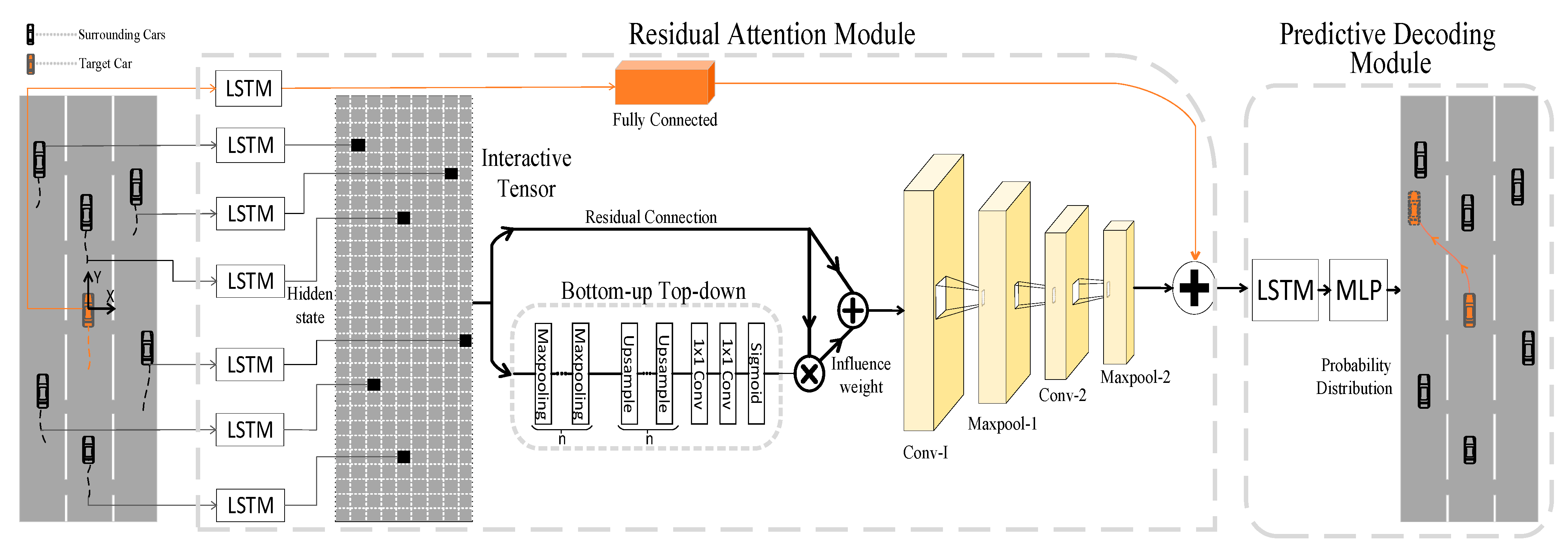
The influence of the interaction between the target vehicle and surrounding vehicles on the prediction accuracy cannot be ignored in the trajectory prediction work. Previous studies [22,23,24,33,34,35,36] seldom considered this influence, and over-relied on the complex relationship in the target vehicle’s historical trajectories. Considering specific scenarios such as highways, Sun Ying [39] and others proposed the fusion of the features of lane lines, target vehicles and historical trajectory data to enhance the correlation between trajectory features and context, and improve the accuracy of the input information. A. Alahi et al. [40] proposed the social pooling structure, which simulates the interaction between pedestrians by constructing a compact interaction tensor from the hidden vector close to the historical trajectory of pedestrians. However, the interaction features in the tensor were not fully extracted. As an extension of [40], Nachiket Deo et al. [41] and Liu Chuang et al. [42] proposed the extraction of the interaction vector with a convolutional layer instead of a fully connected layer, because the advantage of the convolutional layer in terms of extracting local features can prevent the destroying of the spatial structure of the tensor when extracting the interaction features. The method of A. Alahi et al. [40] simulated pedestrians with the same influence weight, so Wenchao Ding et al. [43] proposed a new vehicle behavior interaction network (VBIN), so that the behavior cues of vehicles can be obtained from the vehicle interactions. By adjusting the weight of other targets on the prediction target, the influence of the surrounding environment on the prediction target is more finely solved.

The authors of [41] constructed an interaction vector based on the encoded latent vector of the historical trajectories and the corresponding position of vehicles, and used a convolutional layer to extract the interaction features between the target vehicle and surrounding vehicles in the interaction vector without bias. The new self-encoding social convolution mechanism proposed by Yu Wang et al. [44] can train the model with unlabeled data in a semi-supervised manner.

However, existing research shows that the vehicle in front of the target vehicle has the most influence on the lateral behavior, rather than all surrounding vehicles. In other words, the interaction weight of the vehicle most related to driving behavior is the largest. Therefore, the interaction features extracted without deviation from the hidden state vectors of all surrounding vehicles may have a large deviation from the actual interaction features between vehicles, which is one of the key problems to be solved.

3. Methodology

The residual attention-based trajectory prediction algorithm (RA-LSTM) is proposed in this paper. Inspired by [22], in this model, a symmetric bottom-up top-down structure consisting of a series of convolution, pooling and inverse convolution is applied to the calculation of the degree of influence of all surrounding vehicles, which allows the model to focus on the movements of all surrounding vehicles by increasing the perceptual field, and then obtain a weight tensor of the same dimension as the input by linear interpolation. Based on this, the motion features of the surrounding vehicles that have a large influence on the target vehicle are enhanced and the motion features of the weakly influenced vehicles are suppressed, so that the model can capture the surrounding vehicle interactions that affect the future driving of the target vehicle at each moment.

The improved overall network architecture is shown in Figure 1, including the historical track coding module, the residual attention module and the predicted track output module. Compared with the traditional LSTM basic network model, the main innovation of this paper is that a residual attention module based on bottom up top down structure is proposed to suppress the interference of the historical trajectory of surrounding vehicles that have little impact on the target vehicle, so as to ensure that the model always focuses on the historical trajectory of surrounding vehicles that have greater impact on the target vehicle.

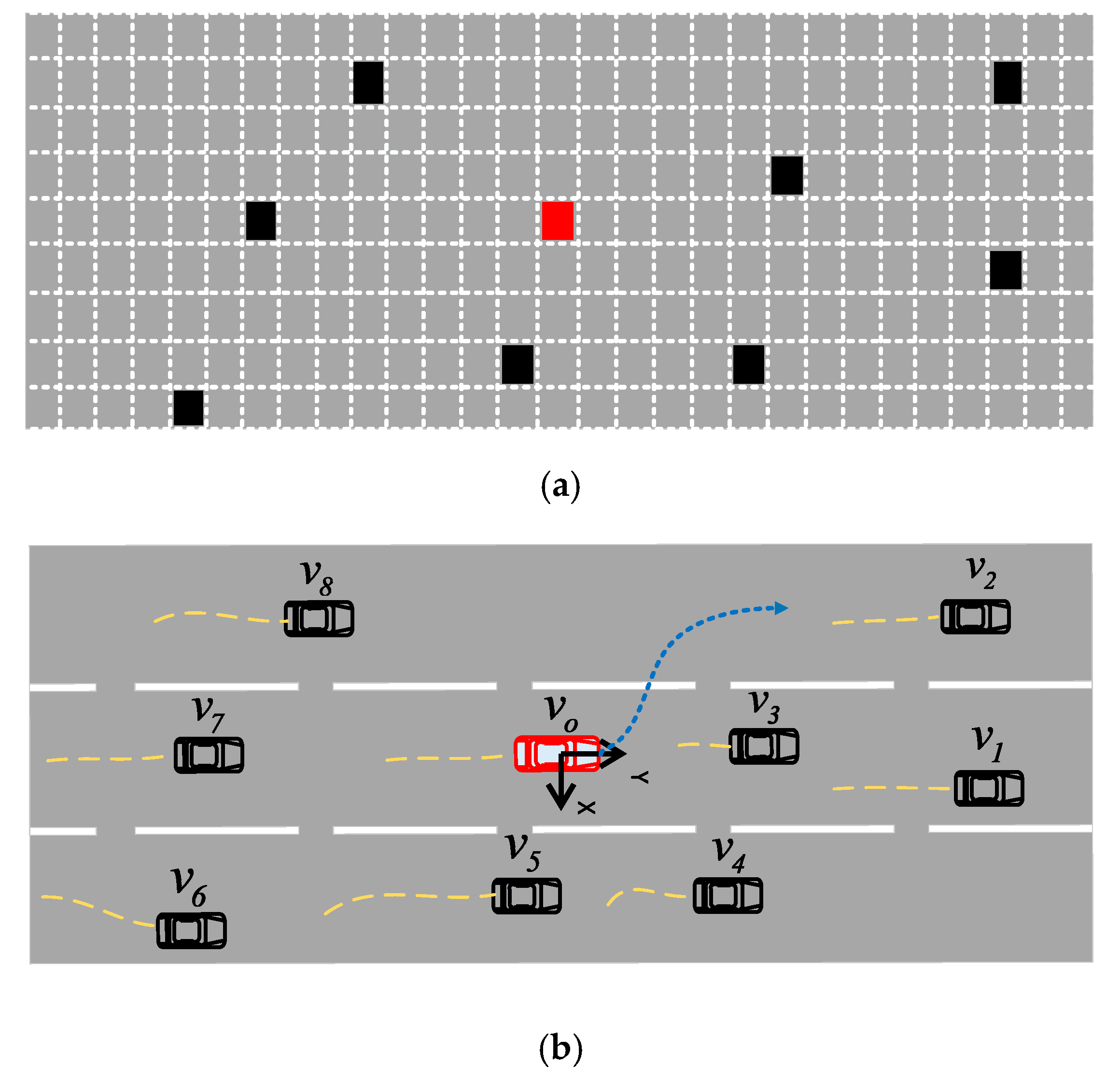
3.1. Research Scenario

The prediction model established in this paper was constructed with aim of studying the task of predicting the future trajectories of moving vehicles on urban structured roads. The predicted trajectory should be as accurate as possible; this puts forward requirements for the generalization ability of the model under various complex road conditions. The movement of the vehicle under complex traffic conditions is mainly influenced by the movements of other vehicles around it and the driver’s intention. The driving intention can be determined by analyzing the historical trajectory of this vehicle, but the influence of surrounding vehicle movements cannot be obtained by analyzing the historical trajectory alone. Therefore, determining the interaction effects of surrounding vehicles is crucial to accurately predict the future trajectory of the target vehicle.

The target vehicle for the trajectory prediction task is defined as $v_o$, and the vehicles around the target vehicle are defined as $v_s\left(s\in 1,2,\dots ,n\right)$; The forward direction of the target vehicle is defined as the positive y-axis direction, the center of the rear axis of the vehicle is the coordinate origin, and the direction perpendicular to the y-axis is the x-axis. Not all vehicles have an impact on the future motion of the target vehicle, just as it is difficult for a driver to pay attention to all vehicles on the road while driving. The scope of the paper study also includes the surrounding vehicles and the interaction behavior occurring between the vehicles close to the target is discussed.

According to the road structure and the effective detection range of the current ADAS system with conventional configuration sensors, the area within the longitudinal (−70 m, 70 m) and three lane area of the target vehicle’s coordinate origin is defined as A, as shown in Figure 2a. It is considered that any influence caused by the surrounding vehicles outside the A area on the target vehicle can be ignored.

3.2. Model Input and Output

At any moment t, the inputs of the trajectory prediction model are the trajectory coordinates of the target vehicle $X_o$ and all surrounding vehicles $X_s$:

$$X_o=\left[\left(x_o^{t-his},y_o^{t-his}\right)\dots \left(x_o^{t-1},y_o^{t-1}\right),\left(x_o^t,y_o^t\right)\right],$$

(1)

$$X_s=\left[\left(x_s^{t-his},y_s^{t-his}\right)\dots \left(x_s^{t-1},y_s^{t-1}\right),\left(x_s^t,y_s^t\right)\right],$$

(2)

The outputs of the model are the coordinates of the target vehicle’s trajectory:

$$Y_o=\left[\left(x_o^{t+1},y_o^{t+1}\right)\left(x_o^{t+2},y_o^{t+2}\right)\dots \left(x_o^{t+pred},y_o^{t+pred}\right)\right],$$

(3)

where his represents the historical observation domain length in the influence domain A, pred represents the length of the future prediction domain in the impact domain A.

3.3. Historical Trajectory Coding

The historical trajectory coding encodes the trajectory coordinates in the historical observation domain of the target vehicle and the surrounding vehicles into hidden state vectors, and fills the hidden state vector of the surrounding vehicles into the corresponding position of the interaction tensor constructed according to the road environment.

In order to uniformly characterize the high-dimensional features in the vehicle trajectory, the input trajectory coordinates in the historical observation domain of the vehicles in region A are mapped to the word-embedding vector $v^t$ via the fully connected layer:

$$v^t=FC\left(X^t;W_{fc}\right),$$

(4)

where $FC()$ is the fully connected layer function and $W_{fc}$ is the weight parameter of the fully connected layer.

The vector corresponding to the historical track is embedded into the implicit state vector of the historical track at the previous time through the LSTM encoder, and we can obtain the current hidden state vector ${\mathit{h}}^t$, which contains the contextual information of the vehicle motion features:

$${\mathit{h}}^t=encoder\left(v^t,{\mathit{h}}^{t-1};W_{enc}\right),$$

(5)

where $encoder()$ is the LSTM encoder, responsible for encoding the word-embedding vector $v^t$ of the vehicle trajectory into a hidden state vector, and $W_{enc}$ is the weight parameter of the encoder.

Finally, the trajectories encoding hidden state vectors of the target vehicle and all surrounding vehicles in area A at the current moment are obtained: ${\mathit{h}}_o^t$, ${\mathit{h}}_s^t\left(s\in 1,2,\dots ,n\right)$.

3.4. Interaction Tensor Filling

In order to characterize the impact of all surrounding vehicles on the target vehicle, it is necessary to combine information about the current spatial location and historical-trajectory context of each vehicle. Inspired by the social pooling aggregated pedestrian spatial and trajectory information proposed by Xu et al. [12], this paper proposes that the interaction tensor of the target vehicle be constructed based on the effective detection distance and lane structure of current advanced driver assistance systems, and the interaction tensor gathers the positional information of surrounding vehicles and the hidden state vector of all vehicles’ historical trajectories.

The area A is specifically divided into [28 × 9] grid areas, with the width of each column of the grid corresponding to 1/3 of the width of each lane, so as to distinguish whether the vehicle is on the left, center or right side of the lane. The height of each row of the grid is 5 m, corresponding to the length of a typical vehicle. The interaction tensor of the same dimension is generated by referring to the grid area; the row number c and column number r of the encoded hidden state vector of the surrounding vehicles in the tensor are calculated based on the offset of the surrounding vehicles relative to the target vehicle position at moment t:

$$\begin{array}{c}c=floor\left(\frac{x_i^t-y_{tar}^t}{\frac{lw}{3}}\right)\\ r=floor\left(\frac{y_i^t-y_{tar}^t}{dc}\right)\end{array}\},$$

(6)

where $c$ = (−4, −3, …, 4), $r$ = (−14, −13, …, 14) and $floor()$ is the function of rounding down; $lw$ is the width of each lane, which, according to the national standard, takes the value of 3.75 m; $dc$ is the line height, with a value of 5 m, which represents the length of a general vehicle.

The coded hidden state vectors of all vehicles in region A at the current moment are filled into the interaction tensor according to the positions found above, and then the interaction tensor $s^t$ of the current target vehicle can be obtained, as shown in Figure 2b.

3.5. Vehicle Interaction Feature Extraction

The interaction features between vehicles can be extracted from the constructed interaction tensor, and the convolutional pooling layer was selected for extraction in [14,21]. In order to represent the difference of surrounding vehicles’ influence, the authors of [20,21] introduced the cosine similarity value and vehicle distance safety distance ratio in the convolutional pooling layer to calculate the influence weight between each surrounding vehicle and the target vehicle, and update the context information on the surrounding vehicles’ historical trajectories according to their weight. However, these methods are based on an ideal assumption made to discuss the influence of surrounding vehicles: surrounding vehicles only interact with the target vehicle, and the movements of surrounding vehicles are independent of each other without interference. Obviously, this assumption is not in line with the real situation under complex traffic road conditions, which will lead to a reduction in the accuracies of predicted trajectories. Thus, inspired by the application in image classification in [22], this paper proposes a bottom-up and top-down structure of the residual attention module to capture the action interactions of all surrounding vehicles and calculate the influence weight of relevant vehicles. The attention module is mainly divided into two branches: Mask and Trunk. The Mask branch focuses on all the vehicle context information in the interaction tensor by gradually increasing the receptive field, and obtains the influence weight of each surrounding vehicle based on the linear interpolation of the related high-dimensional features. The trunk branch is used to pass the original input interaction tensor. Through the dot product of the obtained weight and the interaction tensor transmitted by the trunk branch, the surrounding-vehicle context information that is strongly related to the target vehicle in the tensor is enhanced and the information with weak correlation is suppressed. Then, the vehicle interaction information in the interaction tensor is extracted through the convolutional pooling layer to obtain interaction features that are more consistent with the real driving conditions.

The current target vehicle interaction tensor $s^t$ obtained in Section 3.3 is passed into the Mask branch of the bottom-up top-down structure; after n times of max-pooling, the receptive field is rapidly increased to pay attention to the historical-trajectory context information of each surrounding vehicle in the interaction tensor. After the receptive field of max-pooling covers the global interaction tensor, the extracted high-dimensional features are expanded through the symmetric bottom-up top-down structure, and the feature dimensions are restored to be consistent with the input tensor after n upsampling layers. Finally, the sigmoid activation layer normalizes the up-sampled global features to obtain the influence weight tensor $M^t$ of the surrounding vehicles, as shown in Figure 3:

$$M^t=Upsampl{e}^n\left[Maxpolin{g}^n\left(s^t\right)\right],$$

(7)

Based on the idea of residual learning, the attention module was constructed in the same mapping structure. The original interaction tensor passed by the Trunk branch is dot produced with the weight tensor $M^t$, and then added to the original interaction tensor, which can effectively reduce the weakening effect on the important features in the interaction tensor caused by the error of the vehicle influence weight of the mask branch calculation; at the same time, it also avoids the disappearance of gradients caused by the excessive depth of the network during training, and increases the generalization ability of the model. Thus, the output of the attention module becomes:

$$S^t=\left(M^t+1\right)s^t,$$

(8)

where each element of $M^t$ takes values between 0 and 1, and the new interaction tensor $S^t$ is obtained by dot-multiplying the weight matrix and summing the interaction tensor (if not specifically noted, subsequent interaction tensors are referred to as $S^t$).

Based on the interaction tensor updated with the surrounding vehicles’ influence weights, the interaction features between the target vehicle and the surrounding vehicles are extracted by convolutional pooling layer $e_s$. The features are superimposed with the movement feature $e_{tar}$ of the target vehicle’s historical trajectory to obtain the complete interaction feature $e^t$:

$$\begin{array}{c} e_s=Conv\_pooling\left(S^t\right)\\ { e}_{tar}=dyn\left(h_{tar},w_{dyn}\right)\\ { e}^t=contact\left(e_s,e_{tar}\right)\end{array}\},$$

(9)

where $Conv\_pooling()$ is the convolutional pooling function; $dyn()$ is the MLP (Multilayer Perceptron) layer, used to map the historical hidden state vector of the target vehicle to the motion feature, and $w_{dyn}$ is the weight of the $dyn()$ layer.

3.6. Weight Coefficient of Multilayer Perceptron

The prediction-decoding module consists of an LSTM decoder of the multilayer perceptron. The complete vehicle interaction features $e^t$ extracted from the convolutional pooling layer in Section 3.2. are input to the LSTM decoder together with the decoded hidden state vector ${\mathit{h}}_d^{t-1}$ at the previous moment, so as to obtain the decoded hidden state vector ${\mathit{h}}_d^t$ of the predicted trajectory at the current moment. In order to reflect the randomness of predicted vehicle trajectory points, a multilayer perceptron is used to map the decoded hidden state vector to the probability distribution of the predicted trajectory in the future. The Gaussian distribution is borrowed here, where the mean $\mu =\left({\mu }_x,{\mu }_y\right)$, the variance $\sigma =\left({\sigma }_x,{\sigma }_y\right)$ and the correlation coefficient is $\rho$. The procedure is as follows:

$${\mathit{h}}_d{}^t=decoder\left(e^t,{\mathit{h}}_d{}^{t-1};W_{dec}\right),$$

(10)

$${\theta }^t=\left({\mu }^t,{\sigma }^t,{\rho }^t\right)=mlp\left({\mathit{h}}_d{}^t,w_{mlp}\right),$$

(11)

where ${\theta }^t$ is the Gaussian distribution parameter of the current predicted trajectory, $decoder()$ is the LSTM decoder and $W_{dec}$ is the weight of the parameter in the encoder; $mlp()$ is the multilayer perceptron, and $W_{mlp}$ is the weight of the parameter in the multilayer perceptron.

3.7. Predictive Decoding Module

The weights and bias parameters in the model can be obtained by minimizing the negative log-likelihood loss function training:

$$Los{s}_{NLL}=-\frac{1}{pred}{\sum }_{t_n+1\le t\le t_n+pred}\mathit{log}(P_{{\theta }^t}(Y_o|X_s,X_o)),$$

(12)

where $pred$ is the length of the prediction time domain, and $t_n$ is the prediction-starting moment. $\mu$, $\sigma$ and $\rho$ are the probability distribution parameters of the predicted time domain trajectory points output by the multilayer perceptron in Section 3.3. The data instance of each input model consists of the current target vehicle and the trajectory coordinates within the historical observation domain length of all surrounding vehicles in the affected area A. In order to avoid the gradient disappearance or gradient explosion caused by overly long model input sequences in training, the input trajectory coordinates need to be downsampled uniformly.

4. Experiment

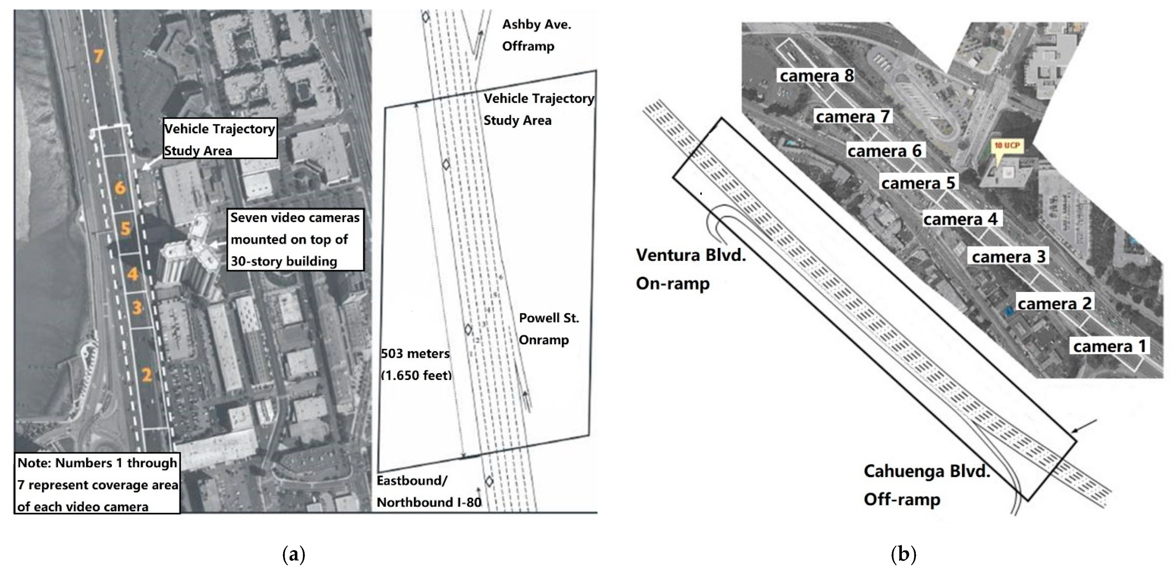
4.1. Data Pre-Processing

In this paper, the I-80 [23] and US-101 [24] road sections from the US public dataset NGSIM (Next Generation Simulation) were selected for the training and validation of the model. The collected road sections are shown in Figure 4; the I-80 dataset was collected on the eastbound Interstate 80 in Emeryville, California. The dataset contains roadway information for the time periods of 4:00 p.m.–4:15 p.m., 5:00 p.m.–5:15 p.m. and 5:15 p.m.–5:30 p.m. The US-101 dataset was collected on the southbound highway 101 in Los Angeles, California, and contains road information during the time periods of 7:50 a.m.–8:05 a.m., 8:05 a.m.–8:20 a.m. and 8:20 a.m.–8:35 a.m. The road information in these two datasets covers three types of traffic conditions: sparse, moderately dense and dense on straight roads. In addition to including a large amount of straight driving condition data, a large amount of scene data on following vehicles and changing lanes were also recorded. Therefore, these two sub-datasets are well suited to the purpose of studying the scenarios of structured road vehicle trajectory prediction.

Since the data structures of the two datasets are similar, the two datasets were treated as the same dataset in the experiment. The information in the original dataset is very rich, but this study only selected what was needed, including the time stamp of the recording time, the vehicle ID number at the corresponding time, and the vehicle’s horizontal and vertical coordinates. Since the original data were not directly recorded by the GPS data that comes with the vehicle, it was derived from the secondary calculation of the detected traffic images by the video processing algorithm, which led to the data containing a certain amount of noise, so the data were filtered using the Kalman filtering algorithm. In order to avoid too many sampling points leading to the disappearance of the LSTM network gradient, the extracted data were downsampled. The acquisition frequency of the original data was 10 HZ, the important features in the data needed to be preserved as much as possible, and the sampling frequency was set to 5 HZ. For the resampled data, the data were extracted with a sliding window of size 8 s to produce samples. For each 8 s, representing a complete data sample, data from the first 3 s were input to the model as historical data and the next 5 s of data were used as the ground truth for predicting the future trajectory. All processed samples were partitioned according to vehicle ID number (vehicle ID number in ascending order according to the time of entering the test section), and all samples were partitioned into a training set, validation set and test set according to the first 70%, 70–80% and 80–100% of vehicle ID numbers.

4.2. Model Training Details

The model was built using PyTorch 1.5.0 with a learning rate of 0.001. The training was performed on a workstation with the Ubuntu 18.04 64-bit OS. For model training acceleration, a GeForce RTX 2080 Ti graphics vehicle was equipped on the workstation and CUDA10.2 was used to accelerate the computation.

4.3. Comparison and Analysis of Experimental Results

(1)

In order to verify the effectiveness of the improved model of this method, the prediction errors of this method were compared with several classical models for the next 5 s under the same historical domain-length trajectory input of 3 s.

①

S-LSTM: A social pooling LSTM proposed in [12], which uses a fully connected layer to extract the interaction between the target vehicle and surrounding vehicles in the original interaction tensor;

②

CS-LSTM: A convolution Social pooling LSTM proposed in [14], which uses a convolutional pooling layer to extract the interaction between the self-vehicle and surrounding vehicles in the original interaction tensor;

③

RA-LSTM: The Res-attention LSTM proposed in this paper introduces the residual attention module to calculate the influence weights of all surrounding vehicles in the influence domain area A to improve the accuracy of extracting the interactive features of surrounding vehicles at each moment.

(2)

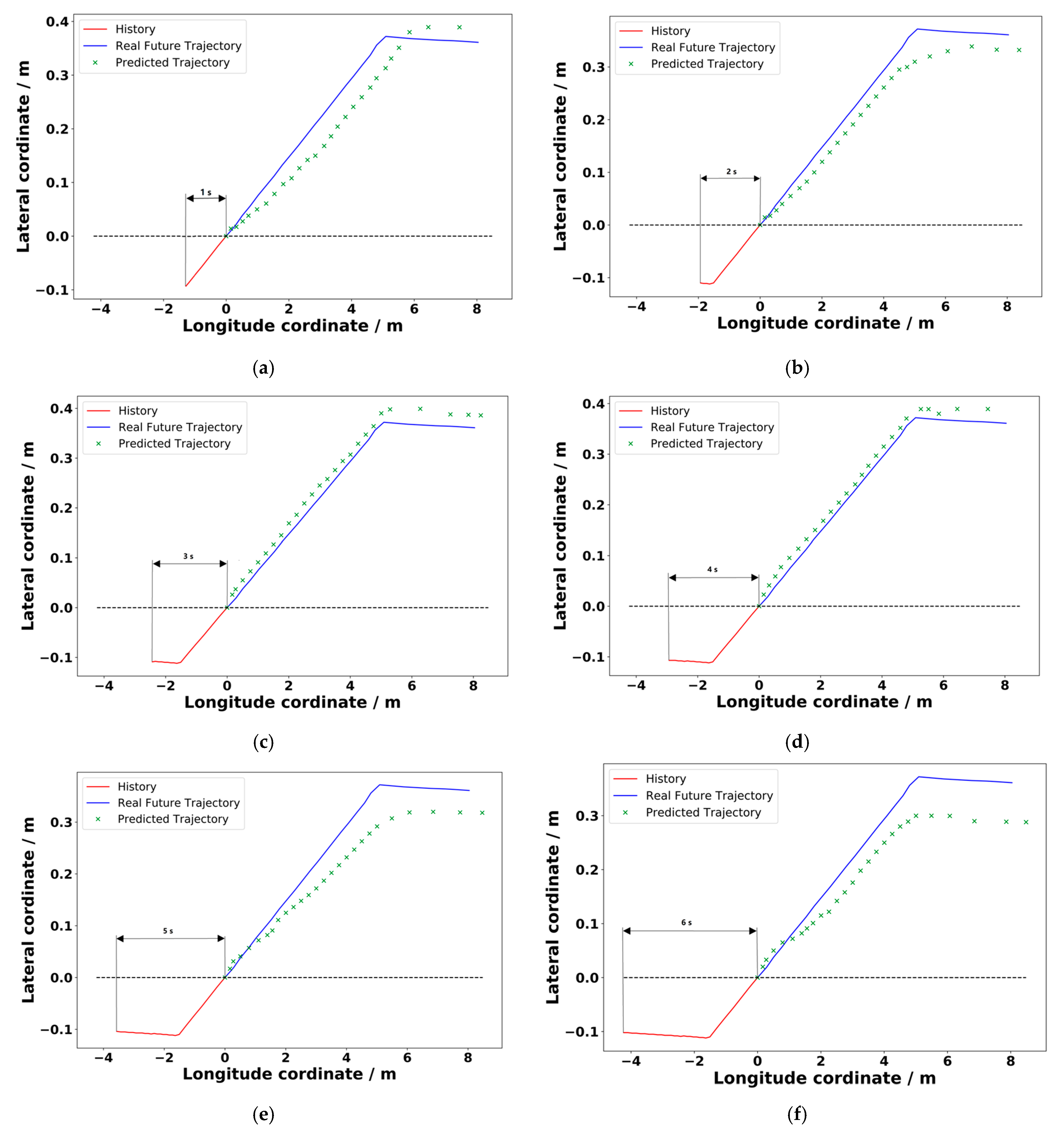
The history domain length of the model input trajectory has a large impact on the accuracy of the future predicted trajectory; The interaction between the self-vehicle and the surrounding vehicles cannot be extracted from an overly short trajectory history, and an overly long trajectory history will lead to a computational stress disaster. In order to determine the optimal historical domain length of the model, the prediction deviations of this method under different domain lengths of historical trajectories were compared and the predicted trajectories were visualized.

4.3.1. Model Performance Comparison

The prediction performance of RA-LSTM model was compared with two popular models: S-LSTM and CS-LSTM.

Table 2. Comparison of root mean square error values and maximum likelihood values for each model.

Prediction Time Domain	RMSE			NLL
	S-LSTM	CS-LSTM	RA-LSTM	S-LSTM	CS-LSTM	RA-LSTM
1 s	1.105	1.099	1.099	0.733	0.639	0.422
2 s	2.143	2.134	2.112	1.716	1.587	1.457
3 s	3.311	3.292	3.198	2.628	2.509	2.467
4 s	4.664	4.642	4.551	3.145	3.081	3.0179
5 s	6.248	6.229	6.205	3.577	3.561	3.486

shows the comparison of the RMSE (root mean square error value) and NLL (negative log likelihood value) obtained for three models with input vehicle trajectory history domain lengths of 3 s and output prediction domain lengths of 5 s for the same test set. For the convenience of error calculation, the RMSE settings in the prediction domain were as follows:

$$RMSE=\sqrt{\frac{1}{pred}{{\displaystyle \sum }}_{t=t_n+1}^{t_n+pred}{\delta }_t{}^T{\delta }_t},$$

(13)

where $t_n$ is the prediction-starting moment, $\delta ={(x-{\mu }_x,y-{\mu }_y)}^T$, $\left(x,y\right)$ is the real trajectory point, and the actual predicted trajectory coordinates are represented as the mean value $\left({\mu }_x,{\mu }_y\right)$ of the future trajectory distribution output of the model.

Obviously, with the improvement of the model, the deviation between the predicted trajectory and the true value became smaller and smaller. The interaction features in the original interaction tensor were extracted by the fully connected layer in S-LSTM, and the interaction information between vehicles could not be fully extracted. The CS-LSTM algorithm improved the method of extracting interactive features using a fully connected layer, and used a convolutional layer instead of a fully connected layer to extract the intersections between vehicles. Compared with S-LSTM, the generalization ability of the model was enhanced, and the trajectory prediction effect was improved. Compared with CS-LSTM, RA-LSTM introduced the attention module of residual connection. The residual attention module of the bottom-up top-down structure was found to be able to pay attention to all the vehicles around the target vehicle, and calculate the global influence weight of each surrounding vehicle.

The interaction tensor was reconfigured according to the calculated weight tensor, so as to suppress the interaction features in the interaction tensor that have less influence on the target vehicle and enhance the effectiveness of the extracted interaction features. Residual connection made it easier to train the model, and avoided the influence of the calculated wrong-attention weight on the feature extraction, which made the model converge faster. The actual prediction results show that the RA-LSTM has higher prediction accuracy than the two algorithms before improvement, which shows that the attention module based on the residual connection plays a positive role in the extraction of real interaction features between surrounding vehicles. Figure 5 visualizes the NLL error values in Table 2, which shows that the improved algorithm had smaller prediction errors and more accurate prediction trajectories as the prediction time domain increased.

4.3.2. Impact of Historical Duration on Forecasting Results

In order to further explore the influence of historical input trajectory duration on the vehicle interaction features extracted by the trajectory prediction model, qualitative and quantitative analysis of the model prediction effects under different input durations was performed. The RA-LSTM model can be given 1 s, 2 s, 3 s, 4 s, 5 s, 6 s historical trajectory input, and analyzed in combination with

Table 3. Comparison of historical trajectory model errors of each length.

Loss Value	History Input Track Length /s
	1 s	2 s	3 s	4 s	5 s	6 s
NLL	3.593	3.557	3.498	3.497	3.581	3.614
RMSE	6.411	6.357	6.205	6.195	6.615	6.898

and Figure 6. From Figure 6a–d, it can be seen that the deviation between the predicted trajectory and the real trajectory gradually decreased with the increasing of the model input’s trajectory history from 1 s to 4 s, which shows that the addition of historical trajectories positively contributed to the extraction of vehicle interaction features. However, when the history domain length increased to 5 s and 6 s, the error of the predicted trajectory started to rebound. From the prediction results in Figure 6e,f, it can be seen that the prediction accuracy was not as good as when the history domain length was 1 s and 2 s. From this, it is clear that the trajectory input in the historical time domain does not need to be too long, or the interactive features in the tensor extracted by the model will be affected. After equalization, it is more appropriate to choose a historical field length of 3 s as the model input. Although the model prediction accuracy was higher when the history domain was 4 s long, the deviation of trajectory prediction was less optimized than the input domain was 3 s long, while the time and computational cost were more costly.

4.4. Scenario-Based Analysis

In actual vehicle trajectory prediction task applications, the model is required to receive the trajectory information at the current sampling moment and update the model input trajectory at every moment, so as to realize real-time prediction of the driving trajectory in the next predicted time domain. In order to verify the feasibility of the model proposed in road conditions, a joint simulation test was conducted using Prescan software and Simulink software.

First, we used Prescan to build a test traffic scene, and then fed the vehicle’s trajectory history information in the scene into the Simulink prediction model; the previously trained trajectory prediction model was loaded and the future driving trajectory was output. The test method is shown in Figure 7. Firstly, when building test traffic scenarios in Prescan, it was necessary to set the sampling frequency of information feedback to Simulink. In order to be consistent with the input dimension of the previously trained RA-LSTM model, the sampling frequency was set to 5 HZ and the road was set as a structured three-lane road. The Bézier curve and Lane-change curve were used to build the vehicle driving path, and then we added the test target vehicle and surrounding vehicles to the scene.

The prediction results of CS-LSTM and RA-LSTM at a certain moment under the typical working condition of left channel change were selected for demonstration. The road traffic conditions are shown in Figure 8(1a) and Figure 8(2a), respectively. Taking the position of the target vehicle at the time of prediction as the origin, this study set the road area within 70 m of the three lanes in the same direction. Among them, the red vehicle was the target vehicle, and the black vehicles were its surrounding vehicles. The speed of all surrounding vehicles was set to a constant speed. The target vehicle started to accelerate at the moment before the prediction. The signals input to Simulink were the historical trajectories of the target vehicle and the surrounding vehicles for the 3 s before the predicted moment, then the previously trained CS-LSTM and RA-LSTM prediction models were loaded to output the target vehicle driving trajectory in the next 5 s.

The prediction trajectory of the model in Figure 8 consists of two parts: the yellow area of the variance visualization of the trajectory coordinate distribution and the mean value of the prediction trajectory distribution represented by triangular lines.

In the scene depicted in Figure 8(1a), the acceleration of the target vehicle resulted in a reduction in the distance from the front vehicle. The interfering vehicle 5 in the left target lane was far away. Figure 8(1d) shows the influence weight $M^t$ of surrounding vehicles. At this time, the influence weight of the front vehicle established by the model was the largest. The influence weight of target lane interference vehicle 5 was small, and the influence on the predicted trajectory of target vehicle was also weak. As can be seen from Figure 8(1b,1c), in this scenario, both CS-LSTM and RA-LSTM could correctly predict the future driving track of the target vehicle, but the prediction distribution variance of RA-LSTM at the end of the prediction track was smaller and the prediction position distribution was more concentrated, reflecting that RA-LSTM has better accuracy in the long prediction time domain.

In the scene depicted in Figure 8(2a), the target vehicle accelerated and the distance between the target vehicle and the front vehicle decreased. At the same time, the longitudinal distance between the interfering vehicle 6 in the left target lane and the target vehicle was small. Combined with the interactive vehicle weight in Figure 8(2d), the target lane interference vehicle 6 exerted the largest influence weight on the target vehicle, and the influence weight of other surrounding vehicles was small. Compared the predicted trajectories of CS-LSTM and RA-LSTM in Figure 8(2b,2c), the effect of RA-LSTM on predicting lane changing trajectories was better than CS-LSTM, because RA-LSTM considered the collision distance with interfering vehicle 6 and increased the influence weight of the attention mechanism. That is to say, the trajectory of RA-LSTM was more consistent with the behavior of skilled drivers. It can be seen that the RA-LSTM model proposed in this paper has more advantages regarding prediction in complex road environments.

5. Conclusions

In this paper, a new residual attention RA-LSTM model focusing on the interactions of surrounding vehicles is proposed. The model innovatively combines the residual attention mechanism in image classifications, the encoder–decoder structure in natural language processing and the convolutional pool structures for interactive feature extractions. In the vehicle trajectory predictive models, the abilities that perceive the interactions of the surrounding traffic environments are enhanced by calculating the interaction weights of the surrounding vehicles and integrating them with the action intentions of the target vehicle. Meanwhile, the extracted interaction features are closer to the vehicle interactions under real road conditions due to the bottom-up and the up-down structures that focus on the behaviors of the surrounding vehicles. On these bases, the NGSIM data set were trained and the virtual sceneries were co-simulated, and the SA-LSTM model was compared with other prediction models. The results show that the proposed model has higher prediction accuracies.

In addition, the SA-LSTM model predicts the driving trajectories without any constraints at present, which means that the actual predicted trajectories are complicated, and it may not be possible in real scenarios. For this reason, the cost evaluation functions, as constraints to improve the drivability of the predicted trajectories, will be considered so that the vehicles’ actions can be predicted more accurately in further studies.

References

1. Barth, A.; Franke, U. Where will the oncoming vehicle be the next second? In Proceedings of the 2008 IEEE Intelligent Vehicles Symposium, Eindhoven, The Netherlands, 4–6 June 2008. [Google Scholar]
2. Ammoun, S.; Nashashibi, F. Real time trajectory prediction for collision risk estimation between vehicles. In Proceedings of the 2009 IEEE 5th International Conference Intelligent Computer Communication and Processing, Cluj-Napoca, Romania, 27–29 August 2009. [Google Scholar]
3. Schubert, R.; Adam, C.; Obst, M. Empirical evaluation of vehicular models for ego motion estimation. In Proceedings of the 2011 IEEE Intelligent Vehicles Symposium, Baden-Baden, Germany, 5–9 June 2011. [Google Scholar]
4. Tamke, A.; Dang, T.; Breuel, G. A flexible method for criticality assessment in driver assistance systems. In Proceedings of the 2011 IEEE Intelligent Vehicles Symposium, Baden-Baden, Germany, 5–9 June 2011. [Google Scholar]
5. Zhang, R. Image Vehicle Motion Trajectory Prediction Method Under Complex Environment. J. Mech. Eng. 2011, 47, 16. [Google Scholar] [CrossRef]
6. Song, X.L.; Xiong, Q.W.; Cao, H.T. Research and Simulation on Cooperative Collision Warning Based on Trajectory Prediction. J. Hunan Univ. 2016, 43, 1–7. [Google Scholar] [CrossRef]
7. Hermes, C.; Wohler, C.; Schenk, K. Long-term Vehicle Motion Prediction. In Proceedings of the 2009 IEEE Intelligent Vehicles Symposium, Xi’an, China, 3–5 June 2009. [Google Scholar]
8. Otto, C.; Leon, F.P. Long-term trajectory classification and prediction of commercial vehicles for the application in advanced driver assistance systems. In Proceedings of the 2012 American Control Conference, Montreal, QC, Canada, 27–29 June 2012. [Google Scholar]
9. Houenou, A.; Bonnifait, P.; Cherfaoui, V. Vehicle Trajectory Prediction based on Motion Model and Maneuver Recognition. In Proceedings of the 2013 IEEE/RSJ International Conference on Intelligent Robots & Systems, Tokyo, Japan, 3–7 November 2013. [Google Scholar]
10. Woo, H.; Ji, Y.; Tamura, Y. Trajectory Prediction of Surrounding Vehicles Considering Individual Driving Characteristics. Int. J. Automot. Eng. 2018, 9, 282–288. [Google Scholar] [CrossRef] [Green Version]
11. Xie, F.; Lou, J.; Zhao, K. A Research on Vehicle Trajectory Prediction Method Based on Behavior Recognition and Curvature Constraints. Automot. Eng. 2019, 41, 1036–1042. [Google Scholar] [CrossRef]
12. Xu, Y.; Xie, J.; Zhao, T. Learning Trajectory Prediction with Continuous Inverse Optimal Control via Langevin Sampling of Energy-Based Models. arXiv 2019, arXiv:1904.05453v. [Google Scholar]
13. Mozaffari, S.; Al-Jarrah, O.Y.; Dianati, M. Deep Learning-based Vehicle Behaviour Prediction For Autonomous Driving Applications: A Review. IEEE Trans. Intell. Transp. Syst. 2019, 23, 33–47. [Google Scholar] [CrossRef]
14. Duan, Y.; Lv, Y.; Wang, F.Y. Travel time prediction with LSTM neural network. In Proceedings of the 2016 IEEE International Conference on Intelligent Transportation Systems, Rio de Janeiro, Brazil, 1–4 November 2016. [Google Scholar]
15. Mikhailov, S.; Kashevnik, A. Car Tourist Trajectory Prediction Based on Bidirectional LSTM Neural Network. Electronics 2021, 10, 1390. [Google Scholar] [CrossRef]
16. Hou, L.; Xin, L.; Li, S.E. Interactive Trajectory Prediction of Surrounding Road Users for Autonomous Driving Using Structural-LSTM Network. IEEE Trans. Intell. Transp. Syst. 2019, 21, 4615–4625. [Google Scholar] [CrossRef]
17. Ji, X.W.; Fei, C.; He, X.K. Intention Recognition and Trajectory Prediction for Vehicles Using LSTM Network. China J. Highw. Transp. 2019, 32, 34–42. [Google Scholar]
18. Hu, L. Research on Autonomous Vehicles Trajectory Prediction Method Based on LSTM; Guilin University of Electronic Technology: Guilin, China, 2021. [Google Scholar]
19. Su, L.M. Research on Trajectory Prediction Method Based on Machine Learning; Beijing University of Posts and Telecommunications: Beijing, China, 2019. [Google Scholar]
20. Khakzar, M.; Bond, A.; Rakotonirainy, A. Driver influence on vehicle trajectory prediction. Accid. Anal. Prev. 2021, 157, 106165. [Google Scholar] [CrossRef] [PubMed]
21. Qiao, Y.L.; Du, Y.P.; Zhao, D.Y. A Location Prediction Method of Markov Based on Gaussian Analysis. Comput. Technol. Dev. 2018, 28, 41–44, 50. [Google Scholar]
22. Xin, L.; Wang, P.; Chan, C.Y. Intention-aware Long Horizon Trajectory Prediction of Surrounding Vehicles using Dual LSTM Networks. In Proceedings of the 2018 21st International Conference on Intelligent Transportation Systems (ITSC), Maui, HI, USA, 4–7 November 2018. [Google Scholar]
23. Wen, H.Y.; Zhang, W.G.; Zhao, S. Vehicle lane change trajectory prediction model based on generative adversarial network. J. S. China Univ. Technol. 2020, 48, 32–40. [Google Scholar]
24. Choi, D.; Lee, S. Comparison of Machine Learning Algorithms for Predicting Lane Changing Intent. Int. J. Automot. Technol. 2021, 22, 507–518. [Google Scholar] [CrossRef]
25. Kim, B.D.; Kang, C.M.; Lee, S.H. Probabilistic Vehicle Trajectory Prediction over Occupancy Grid Map via Recurrent Neural Network. In Proceedings of the 2017 IEEE 20th International Conference on Intelligent Transportation Systems (ITSC), Yokohama, Japan, 16–19 October 2017. [Google Scholar]
26. Sadeghian, A.; Alahi, A.; Savarese, S. Tracking the Untrackable: Learning To Track Multiple Cues with Long-Term Dependencies. In Proceedings of the 2017 IEEE International Conference on Computer Vision, Venice, Italy, 22–29 October 2017. [Google Scholar]
27. Deo, N.; Trivedi, M.M. Multi-Modal Trajectory Prediction of Surrounding Vehicles with Maneuver based LSTMs. In Proceedings of the 2018 IEEE Intelligent Vehicles Symposium (IV), Changshu, China, 26–30 June 2018; pp. 1179–1184. [Google Scholar]
28. Chandra, R.; Bhattacharya, U.; Bera, A. TraPHic: Trajectory Prediction in Dense and Heterogeneous Traffic Using Weighted Interactions. In Proceedings of the 2019 IEEE/CVF Conference on Computer Vision and Pattern Recognition, Long Beach, CA, USA, 15–20 June 2019. [Google Scholar]
29. Amirian, J.; Hayet, J.B.; Pettre, J. Social Ways: Learning Multi-Modal Distributions of Pedestrian Trajectories with GANs. In Proceedings of the 2019 IEEE/CVF Conference on Computer Vision and Pattern Recognition (CVPR) Workshops, Long Beach, CA, USA, 15–20 June 2019. [Google Scholar]
30. Li, F.; Gui, Z.; Zhang, Z. A hierarchical temporal attention-based LSTM encoder-decoder model for individual mobility prediction. Neurocomputing 2020, 403, 153–166. [Google Scholar] [CrossRef] [PubMed]
31. Gao, H.; Su, H.; Cai, Y. Trajectory prediction of cyclist based on dynamic Bayesian network and long short-term memory model at unsignalized intersections. Sci. China Inf. Sci. 2021, 64, 172207. [Google Scholar] [CrossRef]
32. Liang, Y.; Zhao, Z. Vehicle Trajectory Prediction in City-scale Road Networks using a Direction-based Sequence-to-Sequence Model with Spatiotemporal Attention Mechanisms. arXiv 2021, arXiv:2106.11175. [Google Scholar]
33. Khosroshahi, A.; Ohn-Bar, E.; Trivedi, M.M. Surround vehicles trajectory analysis with recurrent neural networks. In Proceedings of the 2016 IEEE International Conference on Intelligent Transportation Systems, Rio de Janeiro, Brazil, 1–4 November 2016. [Google Scholar]
34. Phillips, D.J.; Wheeler, T.A.; Kochenderfer, M.J. Generalizable intention prediction of human drivers at intersections. In Proceedings of the 2017 IEEE Intelligent Vehicles Symposium, Los Angeles, CA, USA, 11–14 June 2017. [Google Scholar]
35. Altche, F.; Fortelle, A. An LSTM network for highway trajectory prediction. In Proceedings of the 2017 IEEE 20th International Conference on Intelligent Transportation Systems, Yokohama, Japan, 16–19 October 2017. [Google Scholar]
36. Park, S.H.; Kim, B.D.; Kang, C.M. Sequence-to-Sequence Prediction of Vehicle Trajectory via LSTM Encoder-Decoder Architecture. In Proceedings of the 2018 IEEE Intelligent Vehicles Symposium (IV), Changshu, China, 26–30 June 2018. [Google Scholar]
37. Rebello, S.; Yu, H.; Ma, L. An integrated approach for system functional reliability assessment using Dynamic Bayesian Network and Hidden Markov Model. Reliability Engineering? Syst. Saf. 2018, 180, 124–135. [Google Scholar] [CrossRef]
38. Leibe, B.; Matas, J.; Sebe, N. Lecture Notes in Computer Science. In Computer Vision—ECCV 2016, Knowledge Transfer for Scene-Specific Motion Prediction; Springer: Cham, Switzerland, 2016; Chapter 42; Volume 9905, pp. 697–713. [Google Scholar] [CrossRef] [Green Version]
39. Sun, Y.; Wang, T. Target Vehicle Trajectory Prediction Algorithm based on Time Series. Automob. Appl. Technol. 2020, 6, 31–33. [Google Scholar]
40. Alahi, A.; Goel, K.; Ramanathan, V. Social LSTM: Human Trajectory Prediction in Crowded Spaces. In Proceedings of the 2016 IEEE Conference on Computer Vision and Pattern Recognition, Las Vegas, NV, USA, 27–30 June 2016. [Google Scholar]
41. Deo, N.; Trivedi, M.M. Convolutional Social Pooling for Vehicle Trajectory Prediction. In Proceedings of the 2018 IEEE/CVF Conference on Computer Vision and Pattern Recognition Workshops, Salt Lake City, UT, USA, 18–22 June 2018. [Google Scholar]
42. Liu, C.; Liang, J. Vehicle trajectory prediction based on attention mechanism. J. Zhejiang Univ. Eng. Sci. 2020, 54, 1156–1163. [Google Scholar]
43. Ding, W.; Chen, J.; Shen, S. Predicting Vehicle Behaviors Over an Extended Horizon Using Behavior Interaction Network. In Proceedings of the 2019 International Conference on Robotics and Automation, Montreal, QC, Canada, 20–24 May 2019. [Google Scholar]
44. Wang, Y.; Zhao, S.; Zhang, R. Multi-Vehicle Collaborative Learning for Trajectory Prediction with Spatio-Temporal Tensor Fusion. IEEE Trans. Intell. Transp. Syst. 2020, 23, 236–248. [Google Scholar] [CrossRef]
Figure 1. Trajectory prediction model based on residual attention.
Wevj 13 00047 g001
Figure 2. Research scenario of RA-LSTM. (a) represents the gridding of lane change scenes; (b) represents a lane change scenario.
Wevj 13 00047 g002
Figure 3. Schematic diagram of mask branching mechanism.
Wevj 13 00047 g003
Figure 4. Sampling section of the dataset: (a) I-80 section; (b) US-101 section.
Wevj 13 00047 g004
Figure 5. Negative log-likelihood values in the 5 s prediction time domain for each model.
Wevj 13 00047 g005
Figure 6. Comparison of prediction results of RA-LSTM model with different lengths of input history trajectories. (af) represent the comparison of the prediction results of the input historical trajectory within 1 s, 2 s, 3 s, 4 s, 5 s, 6 s, respectively.
Wevj 13 00047 g006
Figure 7. Joint simulation test logic.
Wevj 13 00047 g007
Figure 8. Comparison of model predicted trajectory results in joint simulation: (1a,2a) shows the target vehicle lane change trajectory prediction under two different traffic conditions; (1b,2b) shows the predicted trajectory distribution of the CS-LSTM model; (1c,2c) shows the predicted trajectory distribution of the RA-LSTM model; (1d,2d) shows the calculated weight tensor in RA-LSTM, visualizing the weight distribution of the attention influence of surrounding vehicles.
Wevj 13 00047 g008