4.1. Available Sensors and Required Estimations
Control requires information—which can be obtained either through measurement or estimation—about some of the states of the realistic model from
Section 2. With respect to guidance, control relies mainly on the detection of the plastic cones defining the limits of the race track (then used to generate the path to follow), usually achieved through cameras, LiDAR sensors, or a combination of both to compensate for individual shortcomings and achieve a positive redundancy.
In what follows, when the reference is found online to provide obstacle avoidance, it is assumed that cameras and LiDAR sensors provide the information needed to navigate in the track outlined by the cones. On the other hand, when the reference is found offline, in advance, information about some states in a fixed coordinate system is needed. Thus, it is assumed that the position of the vehicle in the global frame could be accessed with the fusion of a GPS system with other sensors (since the GPS alone lacks the necessary accuracy) and its orientation resorting to an appropriate compass or gyroscope. Some of the control strategies used in this scenario will require additional information, such as the rate of change of the lateral error , the lateral velocity , and the yaw rate . The latter could be obtained with an inertial measurement unit (IMU); it was assumed that this sensor was not available, and all these three states need to be estimated.
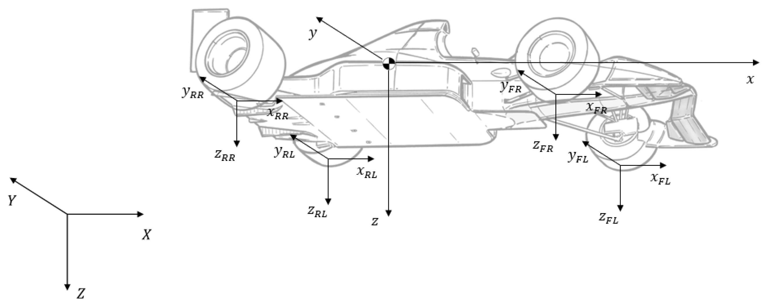
Since we are not here concerned with sensor modelling, sensors were emulated converting the variables in the global frame, obtained from the simulator, into the local frame—the ones provided by the sensors. Considering
and
the coordinates of a given set of points (which could represent, for example, plastic cones) in the global and local frames, respectively, their relation is
where
stands for the coordinates of the local frame origin expressed in the global frame. Thus, from the knowledge of the vehicle’s position
and orientation
, obtained from simulation, the required transformation to obtain a given point in the local reference frame can be obtained by inverting the rotation matrix in (
47) and solving for
.
Speed control will require the feedback of the yaw rate , longitudinal speed , and slip ratio , not available from sensors. Although an accelerometer or a speedometer could provide useful information, the accelerometer is sensitive and noisy, so obtaining through integration is inaccurate; due to the presence of longitudinal slip, the angular speed obtained from the speedometer will not correspond directly to the longitudinal speed of the vehicle. Hence, as no sensor could provide information about the slip ratio, both and are not available and should be estimated; it was simply assumed that they were available for feedback.
4.3. Lateral Control
Lateral control, related to the ability of steering the vehicle to a different lateral position, frequently relies on the knowledge of the vehicle’s pose regarding the track, or in relation to a given referenced path, resorting to variables typically called path-following errors. As such, in this subsection, these variables will be introduced first and then the control strategies will be presented.
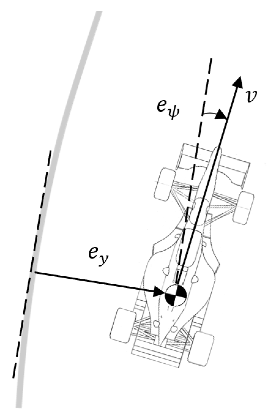
Cross-track and heading errors
In autonomous driving, it is essential to know the vehicle pose in relation to the track in order to allow the control algorithm to correct eventual errors. These can be related to a distance (such as the cross-track error) or an angle (of which the heading error is an example). While it is possible to define such errors in different manners, in this paper, it was assumed that the vehicle has the waypoints in its front, provided by the perception and planning algorithms, and would then curve-fit them with a second-order polynomial in order to obtain a reference path.
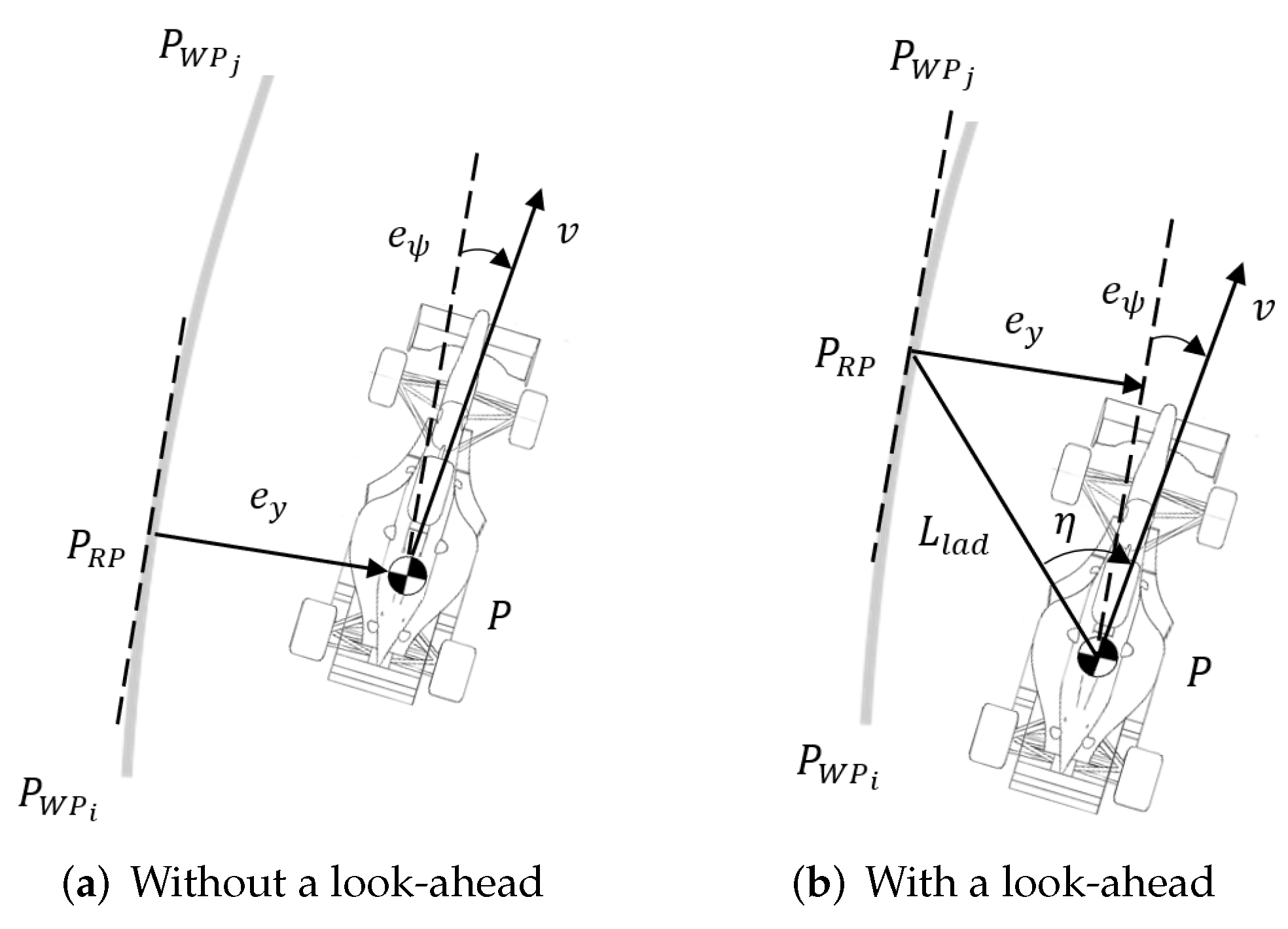
The computation of the path-following errors under this assumption must be done both in the absence and presence of a look-ahead distance
, since such a concept is frequently used for control: indeed, it allows for a timely correction of the errors, providing an anticipation capability. Let
be the reference point to the car expressed in the local frame and
the tangent at that point. The only difference between using or not a look-ahead distance is the location of this point and, consequently, the tangent (as can be seen from
Figure 9). Thus, the mathematical expression for the cross-track error
and the heading error
is the same regardless of the situation. These errors are given by
where the heading error
was defined as the angle between the referenced tangent and the vehicle’s velocity vector
to take into account eventual sideslip. Because both errors are a cross-product of vectors in the
plane, only the
z component of
and
will be different from zero.
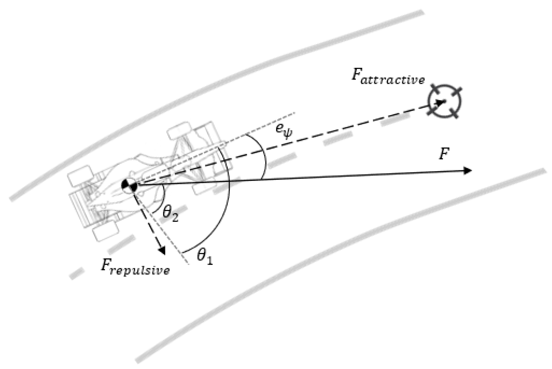
An additional error parameter
that will be used in one of the controllers can also be defined.
is the angle between the look-ahead vector (which can be obtained once the reference point has been established, since its elements will be equal to the coordinates of such point in the local frame) and the velocity vector, as shown in
Figure 9b. This variable can be computed as
and is scalar, for the same reason why errors (
51) and (
52) are, in practice, scalar as well.
Control strategies:
The pure pursuit controller [
34] consists of a nonlinear control strategy, where only one parameter is utilised as the error: the angle
, represented in
Figure 9b.
Assuming a kinematic vehicle model and using a circular arc to connect the rear axle of the vehicle to an imaginary point moving along the desired path, this controller calculates the required steering angle from the curvature of such an arc (obtained geometrically, as shown in [
34]) through
- →
Linear quadratic Gaussian (LQG)
The linear quadratic Regulator (LQR) approach is a linear control strategy. It consists of minimising a given quadratic performance index [
35], which penalises how far the final state of the system is from zero at the end of a finite time horizon and also penalises the state and control authority evolution during the same time horizon. For this minimisation, a significantly good approximation of the optimal solution can be obtained by solving the
algebraic Riccati equation (ARE) [
35], which requires establishing two tuning parameters: the state weighting matrix
, which penalises the state error, and the control weighting matrix
, which penalises the actuation.
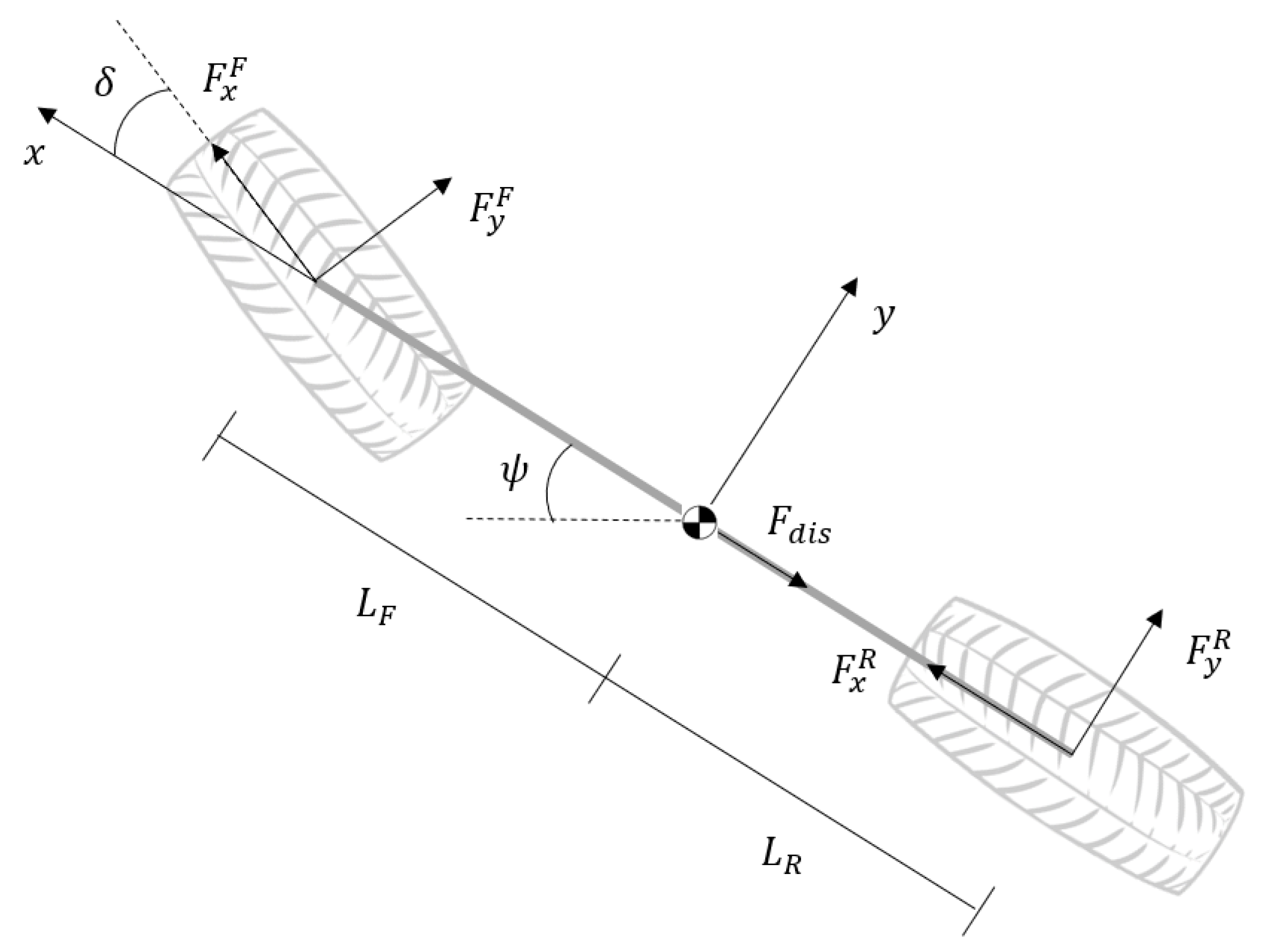
Considering the bicycle dynamics model from
Section 2, the control law is given by
where the gains are obtained from the ARE. Since the model used is parameterised as a function of longitudinal velocity, these gains will be velocity dependent, making it necessary to update them accordingly. This is done resorting to a gain scheduling, where the gains are calculated offline for the speed operating range and then obtained from a neighbourhood table containing these values.
Since variables and are not accessible directly from sensors, the design of a Kalman filter to estimate them is necessary (hence, the designation of LQG). To obtain the gains related to this filter, two additional parameters are needed, namely the process and sensor noise covariances. This estimator uses the same model as the one used for the LQR and resorts, once again, to a gain scheduling to update the gains.
The weighting matrices for the LQR and Kalman filter are
- →
Kinematics lateral speed (KLS)
The kinematics lateral speed controller [
34] is based on the distance between the vehicle and the reference path and on how such a distance should influence the desired rate of change of the cross-track error
: if the car is far from the reference line, it is required to get closer faster than it would get if it were not that far [
34]. As such,
can be defined as proportional to the cross-track error
, with a negative sign. In order to reduce the error between the desired and actual rates of change, the controller must steer the car according to [
34]
where
and
are positive constants and
denotes the curvature of the path at the reference point
, which can be computed by a different definition from the one presented in (
38), since a polynomial was used to curve-fit a given set of waypoints. Let
and
be the coordinates expressed in the local frame of the
n points curve fitted for the reference path generation and
the function describing the second-order polynomial used. Then,
can be computed as
The lowercase letter
k was used, since
is computed with respect to the local frame (while in (
38), the uppercase
K denotes a curvature with respect to the global frame).
The gains used, found with the procedure described above, are and .
This controller (just as MSM below) resorts to a bicycle vehicle model formulated with respect to the path to obtain, from linearisation, a general expression (as in [
34]) for the steering angle, which is then used to obtained the control laws.
- →
Modified sliding mode (MSM)
The sliding mode control strategy is a simple and robust control law, which does not require a precise model of the system [
34]. However, due to the discontinuous nature of its control action, this type of control usually leads to oscillations that are commonly designated as chattering, which can then be be weakened or eliminated. As such, as suggested in [
34], the sliding surface is defined as (
60) and the sliding controller as (
61) in order to ensure stability without chattering.
The resulting modified sliding mode control law can be obtained from [
34]
where
and
are weighting coefficients,
is the curvature at the reference point computed from (
59), and
is given by
Since variable is not directly accessible from sensors, a Kalman filter was designed to estimate it. The model used in this estimator is the bicycle dynamics, written in terms of road errors and, similar to what was done in the LQG controller, resorts to gain scheduling to update the gains.
The weighting matrices for the Kalman filter and the remaining gains used are


