Article

Research on 3D Point Cloud Data Preprocessing and Clustering Algorithm of Obstacles for Intelligent Vehicle

School of Transportation and Vehicle Engineering, Shandong University of Technology, Zibo 255000, China
*
Author to whom correspondence should be addressed.
World Electr. Veh. J. 2022, 13(7), 130; https://doi.org/10.3390/wevj13070130
Submission received: 5 July 2022 / Revised: 18 July 2022 / Accepted: 20 July 2022 / Published: 21 July 2022
(This article belongs to the Special Issue Intelligent Vehicle Control Systems)

Abstract

:
Environment perception is the foundation of the intelligent driving system and is a prerequisite for achieving path planning and vehicle control. Among them, obstacle detection is the key to environment perception. In order to solve the problems of difficult-to-distinguish adjacent obstacles and easy-to-split distant obstacles in the traditional obstacle detection algorithm, this study firstly designed a 3D point cloud data filtering algorithm, completed the point cloud data removal of vehicle body points and noise points, and designed the point cloud down-sampling method. Then a ground segmentation method based on the Ray Ground Filter algorithm was designed to solve the under-segmentation problem in ground segmentation, while ensuring real time. Furthermore, an improved DBSCAN (Density-Based Spatial Clustering of Application with Noise) clustering algorithm was proposed, and the L-shaped fitting method was used to complete the 3D bounding box fitting of the point cloud, thus solving the problems that it is difficult to distinguish adjacent obstacles at close distances caused by the fixed parameter thresholds and it is easy for obstacles at long distances to split into multiple obstacles; thus, the real-time performance of the algorithm was improved. Finally, a real vehicle test was conducted, and the test results show that the proposed obstacle detection algorithm in this paper has improved the accuracy by 6.1% and the real-time performance by 13.2% compared with the traditional algorithm.

1. Introduction

Intelligent vehicles, as the future direction of the automobile field, separate drivers from complex driving operations through advanced technological means [1]. Relying on intelligent vehicles to autonomously perceive the surrounding environment and control the vehicle movement to make up for the lack of driver control of the vehicle plays an important role in reducing the occurrence of traffic accidents, solving traffic congestion problems, and reducing pollution to the environment [2,3]. The intelligent vehicle is a comprehensive intelligent system consisting of four parts: environment perception, positioning, path planning, and control [4]. The environment perception system acquires the surrounding environment information through the perception sensors carried by the intelligent vehicle, which provides a reliable basis for the subsequent positioning and path planning of the intelligent vehicle [5,6].
To achieve omnidirectional, redundant perception of the surrounding environment, most intelligent vehicles are equipped with laser radar, cameras, millimeter wave radar and ultrasonic radar, and other sensors [7]. The cameras have a rich understanding of the environment but are sensitive to light and more difficult to perceive at night or in bad weather, thus limiting their application in driving scenes [8]. Millimeter-wave radar generally operates at a frequency of 77 GHz. The relative velocity of the target can be obtained directly through the phase difference, and the radar can work all day long, but the resolution is low, and the detection effect of small targets is poor [8]. The ultrasonic radar detection distance is only about 5 m, and the signal is greatly affected by the environment [9]. Three-dimensional laser radar is widely used in the environment perception of intelligent vehicles because of its wide field of vision, high resolution of distance and angle, strong anti-jamming ability, independent of illumination, and abundant information obtained about the surrounding environment [10].
Obstacle detection is the most important component of the perception system. At this stage, there are two main detection methods: one is vision-based obstacle detection method, which is susceptible to rain, snow, fog, and other bad weather, and sensitive to light [11]; and the other is an obstacle detection method that is based on 3D radar point cloud data and has strong adaptability to the detection environment [12]. Currently, the commonly used detection algorithms in the field of 3D laser radar target detection include single-frame-based algorithms, multi-sensor fusion, continuous multi-frame-based algorithms, and deep learning algorithms. In general, the above algorithms can be divided into two categories: One is the data statistics class algorithm that can guarantee the algorithm real time; this kind of algorithm is good in real-time, but in the presence of near obstacles, it finds them difficult to distinguish, and it has the problem of splitting long-range obstacles [13]. The other category is the self-learning algorithm with high processing accuracy. In recent years, many scholars have carried out many studies by using this kind of method. Qi proposed a PointNet deep learning network, which directly processes the original point cloud data and segments and identifies obstacles in the three-dimensional space. This method is simple and efficient, but it does not consider the local characteristics and uneven density of point cloud data convolution [14]. Subsequently, PointNet + + and other improved methods were introduced. Yan proposed an improved sparse convolution network based on the problems of slow reasoning speed and poor orientation estimation of 3D convolution network divided by voxels and introduced a new orientation angle loss function and data amplification method [15]. This method is fast and has a good detection effect for large targets. With the continuous development of the deep learning network, an end-to-end neural network has been formed [16] and has been applied in multiple-target detection. However, this method relies heavily on the input point cloud data. Different laser radar wiring harnesses and brands lead to different angular resolutions, making it difficult to adapt to the same network. At the same time, the training of neural network needs a long time, and this brings great pressure to the subsequent decision control module. Self-learning class algorithms have certain advantages in detection performance, but there are more problems in real time which are difficult for real-vehicle applications [17], so how to balance algorithm real time and detection performance has become a research hot spot for related detection algorithms.
To this end, in order to ensure the real time of the algorithm and to solve the problems that the adjacent obstacles are difficult to distinguish and the distant obstacles are easy to split in the traditional obstacle detection algorithm, the first part of this study designed a 3D point cloud data filtering algorithm. Based on this, the second part introduced the design process of ground segmentation algorithm. The third part completed the design of the point cloud clustering algorithm based on improved DBSCAN. The real vehicle validation was presented in the fourth part.

2. D Point Cloud Data Filtering Algorithm Design

2.1. Vehicle Body Point Removal

In order to obtain a larger detection range of radar, the radar detector is generally mounted on the roof of the vehicle through a bracket. According to the vertical angle range of the laser beam emission, there will be some laser points falling on the body of the vehicle that cannot express the characteristics of the surrounding environment and may be mistaken as obstacle point clouds, thus affecting the normal driving of the vehicle; therefore, the vehicle body points need to be removed. Only the measurement points falling within the vehicle body range need to be filtered out according to the length and width of the vehicle and the installation position of the radar; that is, all the measurement points satisfying the following equation need to be filtered out.
L 2 d x L 2 + d
W 2 y W 2
H z 0
where L and W are, respectively, the length and width of the vehicle; H is the radar mounting height; d is the difference distance from the radar center to the center of the vehicle length; x denotes the x-axis coordinate value; and y denotes the y-axis coordinate value.

2.2. Noise Point Removal

The radar is rigidly connected to the vehicle body. Due to the vehicle’s own vibration, the uneven road surface, the interference of radar device characteristics, flying insects, suspended fallen leaves, dust, bad weather, etc., some isolated noise points and outlier points far away from the vehicle are generated in the detected point cloud data. The measurement data of these noise points are useless, and if they are mistaken for obstacles, they will lead to false alarms of the system and affect the normal driving of the vehicle and bring an unnecessary computational burden to the system and reduce the real time of data processing. Therefore, noise points need to be removed before carrying out subsequent point cloud data processing in order to ensure the effective reliability of the data. According to the characteristics of the noise points, in this study, we chose to use statistical filters to remove the noise points.
The filtering process of the statistical filter is given in Figure 1. First, the distance from each point to its nearest neighbor is calculated and the average is obtained. Then, assuming that the obtained results follow a Gaussian distribution, the distance threshold is computed by calculating its mean and standard deviation through the Gaussian function. Finally, the average distance and distance threshold of all points are traversed, and the relationship between them is compared to determine whether the point is a noisy point.
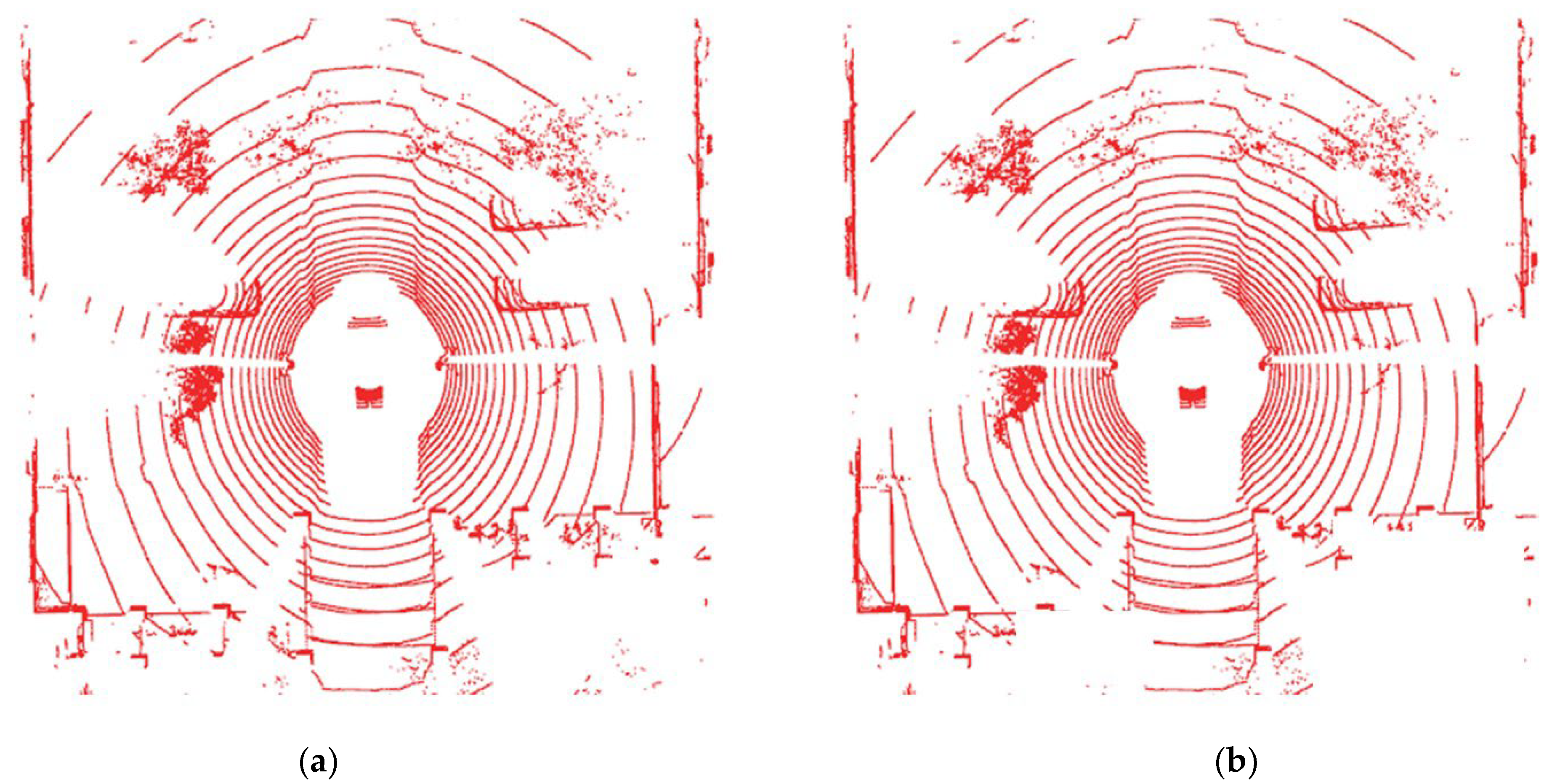
Take a frame of point cloud data as an example and apply the statistical filter to filter out the noise points. A frame of the original point cloud is shown in Figure 2a. There are many discrete noise points in the original point cloud data, and they are mostly distributed in the outer part of the scanning range of the radar. After using the noise-point-removal algorithm designed in this study, an optimized point cloud image shown in Figure 2b is obtained. The results show that the designed algorithm based on a statistical filter can effectively remove the discrete noise points in the distance.

2.3. Point Cloud Down-Sampling

The operating frequency of radar is generally set to 10 Hz, returning hundreds of thousands of laser points per second. Such a large amount of data can consume a large amount of computing resources and reduce the real-time data processing. Therefore, under the premise of ensuring enough useful information, the point cloud is down-sampled to speed up the operation of the algorithm. In this paper, the point cloud down-sampling method uses the voxel grid filter (VGF). The core idea of this method is to create a 3D voxel grid for the point cloud data, set the size of the grid, calculate the number of points within each voxel, and output the center point or the barycenter point of each voxel if the specified number is reached. The retention of information points depends on the size of the voxel division. The smaller the voxel edge length, the more point clouds left, which also affects the computer processing speed. The larger the voxel edge length, the fewer point clouds left, but this may filter out useful data, resulting in incomplete representation of the surrounding environment; thus, a reasonable voxel edge length needs to be chosen for the design. As shown in Figure 3a, a frame of the original point cloud map is collected with a very large number of point clouds. Figure 3b,c gives the effect after filtering with voxel grid filters of different voxel edge lengths. The results show that, when the voxel edge length is set to 0.2 m, the number of point clouds is significantly reduced, but it can still represent the obstacle contour information completely and improve the execution speed of the algorithm. When the voxel edge length is set to 0.3 m, the number of point clouds is further reduced, and the information of some useful points is filtered out, thus resulting in incomplete representation of obstacle contour information, which affects the subsequent detection processing. Therefore, in this study, when using the voxel grid filter to filter the point cloud, the selected voxel edge length was set to 0.2 m.

3. Design of Ground Segmentation Algorithm for 3D Point Cloud Data

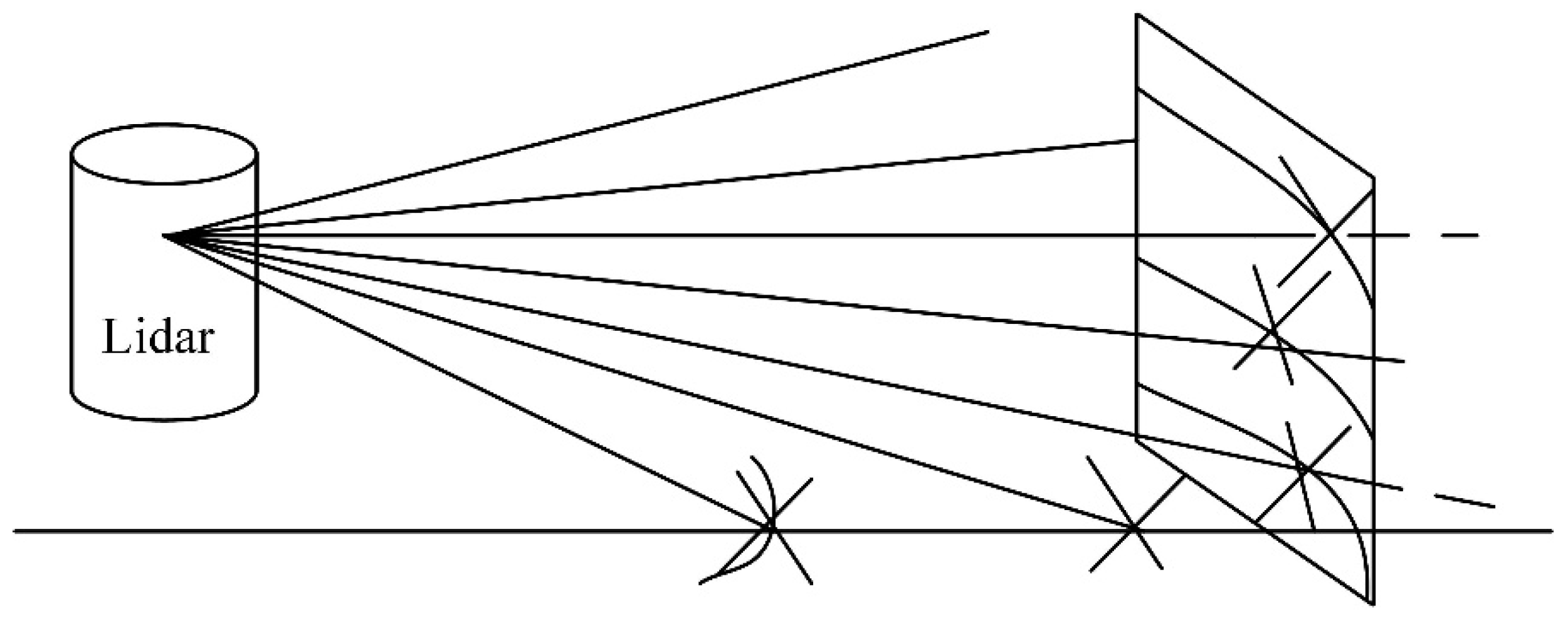
In this study, the Ray Ground Filter algorithm was adopted to segment the Ground point cloud. The core of the algorithm is to process the point cloud in the form of Ray. Firstly, the point cloud is cut according to the height, and the high areas are ignored, and the points close to the car body are filtered out. Then the three-dimensional point cloud coordinates are transferred to the two-dimensional space plane, and the horizontal range of 360 degrees is differentiated. The radar used by the sample vehicle in this experiment has a horizontal angular resolution of 0.16 degrees and can be equally divided into 2250 parts, each of which is connected to the center of the radar to form a ray. The longitudinal section of the radar is shown in Figure 4. Thirty-two laser emitters are distributed up and down in the vertical field of view of the radar. They emit the laser beam shown in the picture. Thirty-two laser beams are projected onto the ground at the same horizontal angle to form a ray.
In order to process laser beams in the same angle, point cloud data need to be converted from a rectangular coordinate system to polar coordinate system.
r = x 2 + y 2
θ = arctan y x × 180 π
where r represents the horizontal distance from the point to the radar center, and q is the included angle between the point and the front of the vehicle.
The segmentation principle of the Ray Ground Filter algorithm is that the height values of ground points and non-ground points scanned by the points before and after the same ray are obviously different. The height difference between the points to be judged and the two points before and after the ray and the height values of the points to be judged are used for ground segmentation. The main steps are as follows:
Step 1: Firstly, sort the points on the same ray according to the distance, calculate the horizontal distance between the points and the radar, preset the slope threshold ( S L , S G ) of two adjacent points of the same ray and the whole ground, and set it as 8°and 5°.
Step 2: Calculate the local and global height thresholds ( H L and H G ) according to S L , S G , and the horizontal distance from the point to the radar, and then calculate the height difference between the current point and the previous point and the height threshold, so as to judge whether the current point is a ground point. When Δ z H L , if the previous point is an off-ground point, further judgment needs to be made according to H G . If the height of the point is greater than H G , it is an off-ground point; otherwise, it is a ground point. If the previous point is the ground point, then this point is the ground point. When Δ z > H L , the height of the point is less than H G , so it is a ground point; otherwise, it is a non-ground point.
Step 3: Update the information of the current point. After judging the current point, traverse all ray points in order to separate ground points from non-ground points.
As shown in Figure 5, ground segmentation effects under different algorithms are given. Figure 5a shows a frame of original point cloud scanned by radar. Figure 5b is the effect diagram after ground segmentation using the RANSAC algorithm, where red represents the ground point cloud and blue represents obstacle point cloud. In order to ensure the real-time performance of the algorithm, the number of iterations set by the algorithm is small, resulting in the under-segmentation of the ground point cloud in the orange box in the figure, which is mistakenly detected as the obstacle point cloud. Figure 5c shows the ground segmentation effect after applying the design method in this paper. The results show that the ground point cloud is completely segmented, and the method also meets the real-time requirements.

4. Design Based on Improved DBSCAN Point Cloud Clustering Algorithm

4.1. Design of Region Growing Algorithm

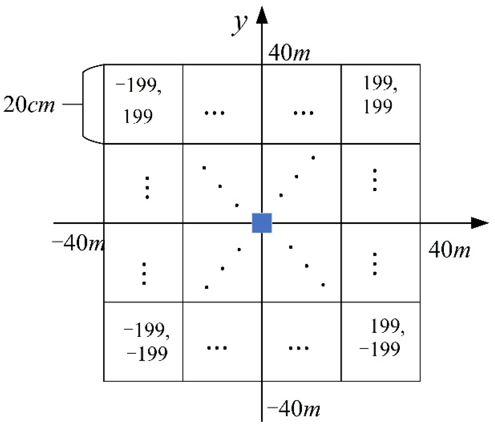
In order to facilitate the processing of the clustering algorithm, the point cloud data within the range of 40 m before and after the intelligent vehicle were rasterized in this study. As shown in Figure 6, a grid of 400 × 400 size was created based on the vehicle coordinate system, and each grid was divided into 20   cm × 20   cm size. The grid map can represent the plane of the vehicle in the form of grid. Then the point cloud data were made to correspond to the grid to determine whether the grid area was occupied. Finally, the point cloud data in the occupied grid were clustered to determine the scope of the obstacle in the grid map and the relative orientation of the vehicle. The grid division is smaller, and the higher the expression accuracy of the map is, the larger the calculation amount is. In this study, considering the perception accuracy and the calculation speed of the clustering algorithm, the grid map of 400 × 400 was established based on the vehicle coordinate system. Each grid was divided into 20 cm × 20 cm, and the point cloud data in the 40 m area around the vehicle were processed. The algorithm needs to record the number of point clouds in each grid, the maximum and minimum height difference of point clouds, and the traversal identification value.
Region growth is a continuous region segmentation algorithm in computer vision. The basic idea is to collect pixels with similar quality and form a region. On the premise of ensuring good edge information, the algorithm can cluster the point cloud data, extract the connected regions with the same characteristics, and complete the clustering of obstacles. The specific steps are as follows:
(1) Select the seed spot. According to Equation (6), the height difference in each grid is calculated, and the obstacle grid whose height difference is larger than the height difference threshold is selected as the seed grid. In this paper, the height difference threshold is 0.3 m.
Δ h = G h G l
where Δh is the height difference, and Gh and Gl are the maximum and minimum height of points in the grid, respectively.
(2) Conduct 8-neighborhood expansion with seed points. Since the maximum height value of the same obstacle in adjacent grids is close, the grids satisfying Formula (7) in the 8-neighborhood search are added to the obstacle list; the grids that have not been visited in the list are regarded as a new seed grid. Moreover, the searches are continuing in order to determine whether the unvisited grid is the same obstacle. When all grids in the list are visited, the clustering of a single obstacle is completed.
G i _ h G j _ h T c h
where G i _ h and G j _ h are the maximum heights of the inner points of adjacent grids i and j, respectively.
(3) All obstacles can be clustered by sequentially visiting all the remaining unvisited rasters.

4.2. Design of Improved DBSCAN Fusion Region Growing Algorithm

The region growing algorithm’s clustering speed is fast, but the accuracy is low. The improved DBSCAN algorithm can solve the splitting problem of distant obstacles and separate nearby obstacles, but it takes a long time. Therefore, this paper fuses the two detection algorithms to obtain a clustering algorithm with high real-time performance and accuracy. The specific steps of the algorithm are as follows:
(1) Determine the seed grid. According to Equations (6), (8) and (9), the maximum height difference, center of gravity, and variance in each grid are calculated, respectively. It was determined that the grid with variance greater than the threshold value contained different obstacles, and the grid with height difference greater than the threshold value was selected as the seed grid.
C i = 1 n j = 1 n p j
σ i = 1 n j = 1 n ( C i x p j x ) 2 + ( C i y p j y ) 2
where C i is the center of gravity of the grid, p j represents the data points in the grid, and σ i is the variance.
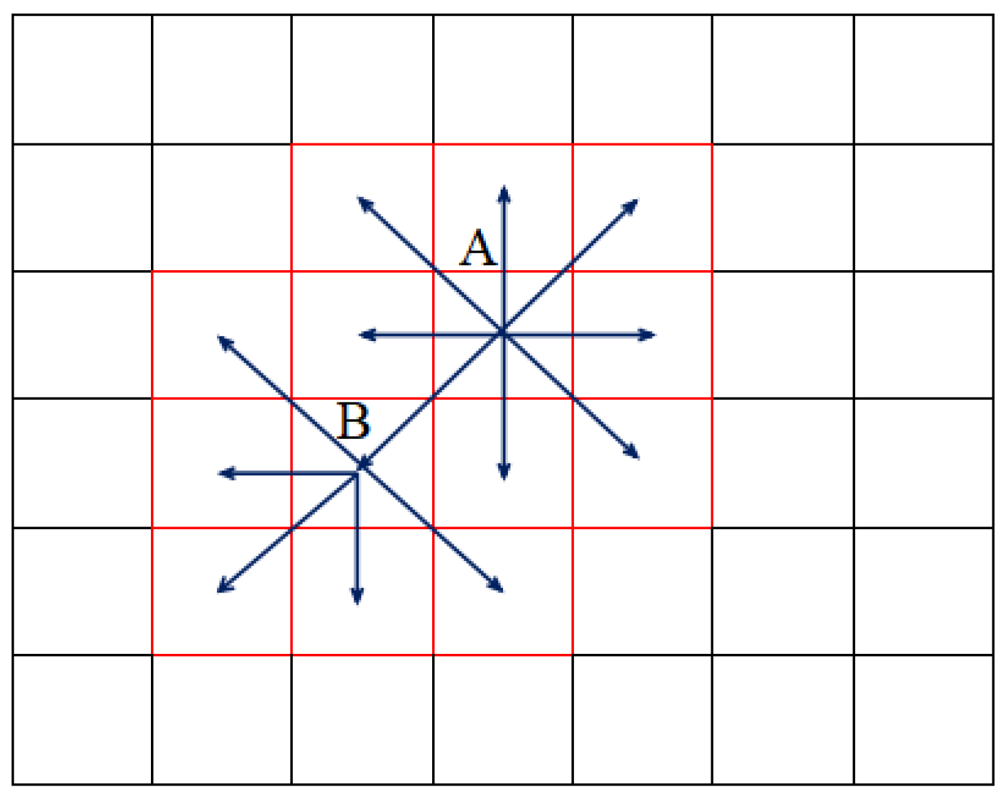
(2) Conduct 8-neighborhood expansion clustering. As shown in Figure 7, the 8-neighborhood searches are carried out counterclockwise, with point A of the seed grid as the center. After visiting the surrounding grids, the next grid point, B, is used as a new seed grid, and the 8-neighborhood searches continue until all grids have been visited and a single obstacle is detected. Repeat the above steps for the remaining unvisited grids to complete the detection of all obstacles.
(3) Execute the improved DBSCAN algorithm. After the second step of clustering, if the obstacle contains the marked grids of multiple obstacles and the volume satisfies Formula (10), the DBSCAN algorithm that adaptively determines the clustering parameters is executed on the obstacles to solve the problem. The distant obstacles are divided into multiple obstacles, and the nearby obstacles are difficult to distinguish; thus, the accuracy of clustering is improved subsequently.
{ o b g _ n T g _ n o b m _ n T m _ n
where o b g _ n is the number of grids contained after obstacle clustering; o b m _ n is the number of grids containing multiple obstacles after clustering; and T g _ n and T m _ n are the grid number threshold and multi-barrier grid number threshold required by obstacle clustering, respectively. This article takes 16 and 5 for the two values.
The steps of the DBSCAN algorithm for adaptively determining the cluster parameters are as follows:
(1) The K-means algorithm is first performed on the dataset. This method is not used to obtain the final clustering result, but to group the data through several simple iterations without increasing the computational burden of the system. The DBSCAN algorithm needs to calculate the distance between each point in the data set and all other points to determine whether it is a core point; this process will consume a lot of computation. In this method, each group is calculated separately after grouping, and the considered range is smaller, which can greatly reduce the time spent judging whether it is a core point.
(2) The point cloud data obtained by radar is near dense and far sparse. In order to complete the clustering better, the neighborhood radius, Eps, should be adjusted so that it can better cluster targets at different distances. Since the horizontal angular resolution of radar is constant, when the laser beam sweeps to the same obstacle, the distance value of two adjacent points should be very close. According to Formula (11), the neighborhood radius can be automatically adjusted according to the distance:
E p s = λ π Δ α D i 180 °
where Δ α is the horizontal angular resolution of the 32-line radar, which is 0.16°; Di is the horizontal distance from the i-th point to the origin of the radar and l is the neighborhood radius coefficient. According to the experiment, this paper takes 1.3.
(3) After executing the DBSCAN algorithm for each group of data, consider whether the data on the boundary of adjacent groups belong to the same class. Check the distance between groups: if the distance is greater than the specified distance threshold, it is impossible to merge the boundary data of the two groups, and there is no need to check the cluster merge within the group; and if the distance between groups is less than the distance threshold, the possibility of clustering combination within the group is analyzed. If the distance between clusters is less than the distance threshold, the possibility of clustering combination can be combined; otherwise, the possibility is zero. Merge clustering is performed by re-executing the DBSCAN algorithm.

4.3. Bounding Box Fitting

After the clustering is completed, the candidate objects to be tracked are obtained, and the size of the clustering is calculated by Formula (12). In order to describe the location, size, and orientation of obstacles and enhance visual features, the point cloud data of the obstacles is surrounded by a 3D bounding box, so that it has uniform dimensional information and heading. The bounding box is also called the minimum circumscribed 3D box, which is used to determine minimum bounding space for discrete data points. Considering that there are many people and vehicles in the road environment, and there are relatively few objects with complex shapes, and considering the real-time processing of laser point cloud data, cuboids that are easy to create are selected as boundary boxes. Usually, the Minimum Area Rectangle (MAR) method is applied to each clustered object to obtain a 2D box, which is combined with height information to form a 3D bounding box.
{ l n = Y max n Y min n d n = X max n X min n h n = Z max n Z min n V n = l n d n h n
where X max n , X min n , Y max n , Y min n , Z max n , and Z min n are the maximum and minimum values of the XYZ coordinates of the nth cluster, respectively; ln, dn, hn, and Vn are the length, width, height, and volume of the nth cluster, respectively.
The MAR method is suitable for fitting the boundary of obstacles parallel to the coordinate axis, but it cannot guarantee that the fitting direction of the partially occluded obstacle is correct, and when the obstacle is not parallel to the coordinate axis, the generated 3D rectangular frame cannot fit the edge of the obstacle well. Therefore, this paper adopts the feature-based L-shaped fitting to derive the correct fitting direction. The process of L-shaped fitting is as follows:
First, select the outliers, a and b, that are farthest from both sides of the obstacle boundary facing the radar. Then connect points a and b to obtain line segment, Ld (all points in the obstacle make an orthogonal line to Ld), and use the iterative endpoint fitting algorithm to find the line segment with the largest distance and the angle close to verticality as L0. Finally, let the corner point where L0 does not intersect with Ld becomes c and connect the three points, a, b, and c, to get an L-shaped polyline, as the line segment bc shown in Figure 8. Since the heading of most vehicles is parallel to the longest side of the boundary, the heading of the bounding box is the longest line segment. This method requires enough data points and is mainly designed for obstacles in the shape of a cuboid. Therefore, compared with smaller obstacles, such as bicycles and pedestrians, it is more suitable for automobile obstacles and can also deal with the case of occlusion.
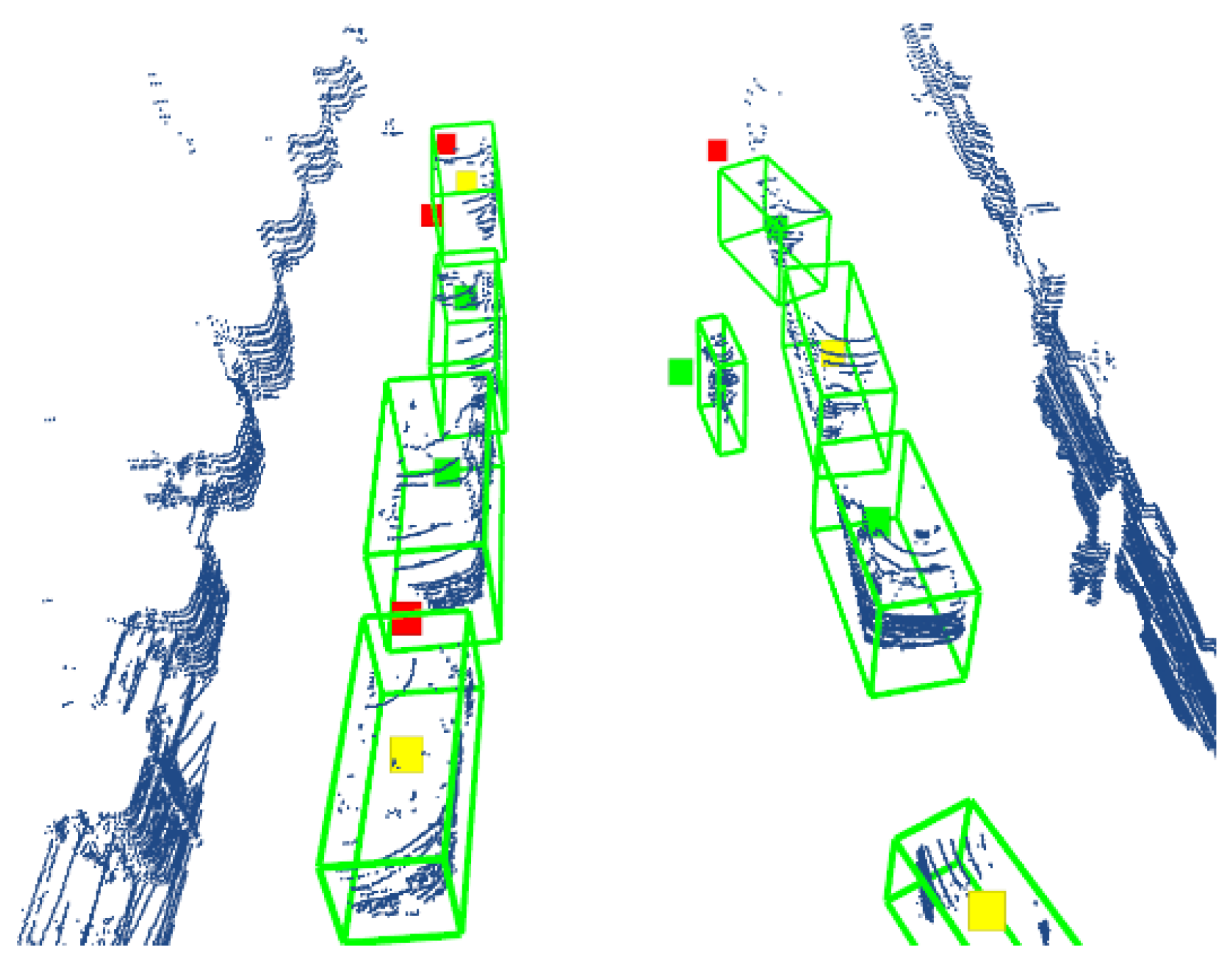
After the heading of the obstacle and the 2D bounding box are determined by the above L-shaped fitting, the height of the 3D bounding box is determined by the maximum height difference in the obstacle point cloud. In combination with height, the rectangular box generated by this method is shown in Figure 9. It is obvious from the figure that 3D bounding boxes of the vehicles on both sides of the road are well fitted.

5. Experimental Verification

5.1. Analysis of Point Cloud Preprocessing Experiment

Figure 10a is a frame of raw radar data captured in RVIZ, including vehicles, pedestrians, trees, and buildings, where the concentric circles represent the ground points. Figure 10b is the point cloud image obtained after filtering the original point cloud. The number of point clouds is obviously reduced, but the useful information of the point cloud is basically retained, which can reduce the amount of calculation of data processing and improve the real-time performance of the system. Figure 10c is a frame of obstacle point cloud image obtained after dividing the ground by using the Ray Ground Filter algorithm. The number of point clouds is further reduced, and the ground points are completely removed. After the above point cloud filtering and ground segmentation operations, a frame of valid point cloud data is obtained, and on this basis, the subsequent point cloud clustering and target tracking process are more accurate.

5.2. Analysis of Point Cloud Clustering Experiments

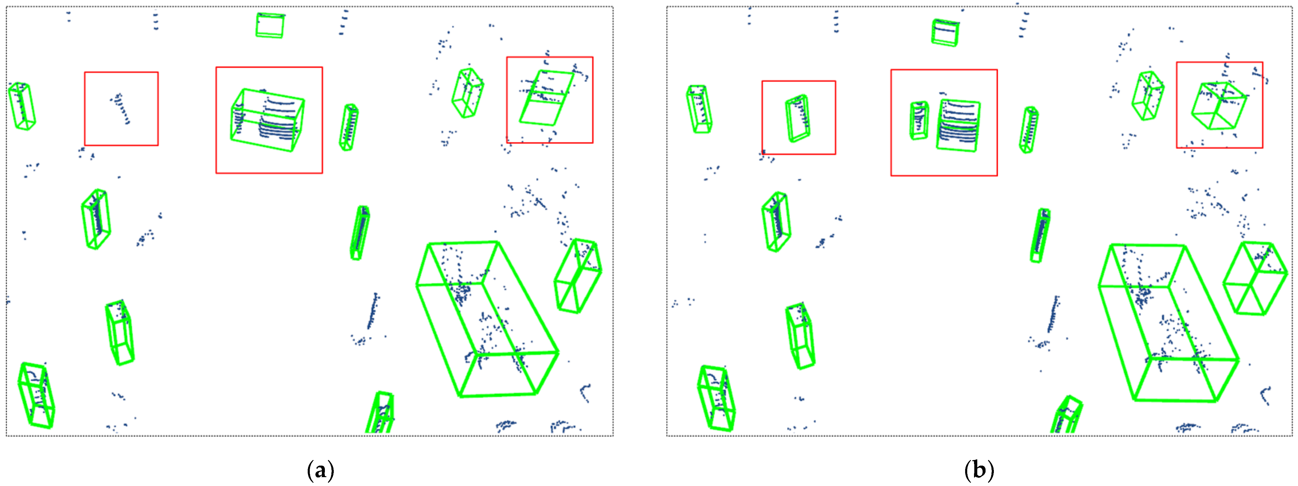
In order to verify the effect of the improved DBSCAN fusion region growth algorithm designed in this paper, multi-target detection experiments at different distances were carried out on the experimental vehicle, and a total of 500 frames of point cloud data were collected. The average speed of the experimental vehicle is in the range of 20–30 km/h. The clustering result of the point cloud near the obstacle of the smart car is given in Figure 11. The obstacles acquired by the radar in the test environment are mainly vehicles, pedestrians, and trees on the roadside. The traditional DBSCAN algorithm fails to detect the collected point cloud data and fails to cluster the trees on the roadside. In addition, since the clustering parameters are fixed, the clustering results are inaccurate, and the adjacent vehicles and pedestrians cannot be distinguished; thus, they are integrated and regarded as a target. Based on the improved DBSCAN fusion region growing algorithm, all obstacle point clouds can be clustered without missing detection. At the same time, the vehicles and pedestrians are clustered and distinguished, and the outline of obstacles can be detected more accurately.
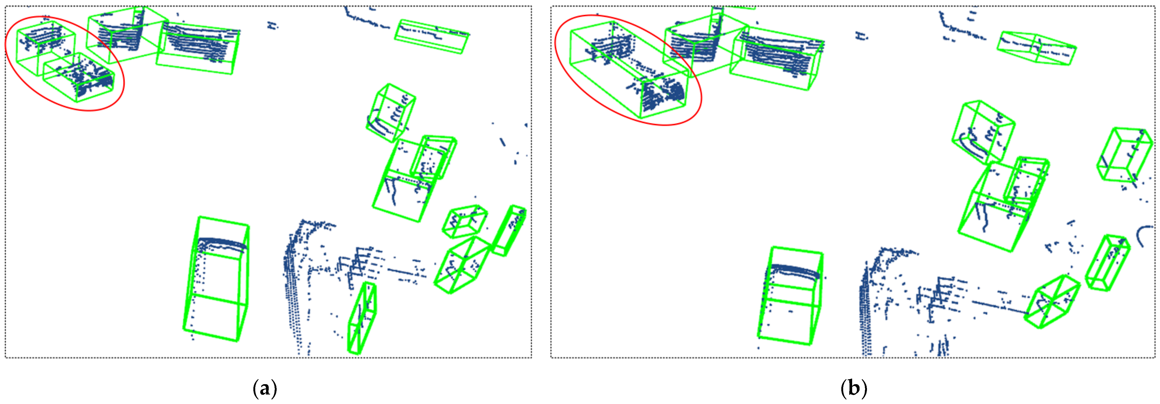
The clustering result of the point cloud near the obstacle of the smart car is given in Figure 12. There are obstacles such as large trucks, ordinary vehicles, and roadside vegetation in the test environment. As the clustering parameters of the traditional DBSCAN algorithm remain unchanged, a truck is split into two different obstacles during the clustering process. The improved clustering method can well cluster the distant sparse obstacle point cloud and completely detect the truck. To sum up, the improved method in this paper can solve the problems that adjacent obstacles are difficult to distinguish and distant obstacles are split; it also has qualified detection results for obstacles at different distances, this improving the driving safety of smart cars.
In order to further verify the accuracy and real-time performance of the method, the collected 500 frames of point cloud data were preprocessed, and on this basis, the traditional DBSCAN algorithm and the improved method were used for clustering. In order to evaluate the clustering effect, the number of accurately detected obstacles and the total number of obstacles in the data collected in each frame were recorded manually, and the ratio of the two was used as the positive detection rate. Finally, the average value of the positive detection rate of 500 frames was used as the clustering evaluation standard. The test results show that the improved clustering method enables the adaptive determination of clustering parameters with the detection distance, making it better than the traditional DBSCAN algorithm; it reduces the false detection and missed detection of obstacles and increases the average positive detection rate by 6.1%. In addition, due to the fusion of the region growing algorithm, the data processing time is shortened by 13.2%.

6. Conclusions and Future Work

In order to solve the problem that the adjacent obstacles are difficult to distinguish and the distant obstacles are easy to split in the traditional obstacle detection algorithm, obtain more accurate surrounding environment information, and improve the driving safety of intelligent vehicles, this study improved the traditional obstacle detection algorithm. Through real vehicle experiments, the effectiveness and real-time performance of the improved algorithm were verified. By designing the point cloud data removal of the body points and noise points of the smart car and optimizing the point cloud down-sampling method, the amount of point cloud data of the smart car can be reduced, and the real-time performance of the system can be improved. Based on the Ray Ground Filter algorithm, we can solve the problem of under-segmentation in ground segmentation. The traditional DBSCAN clustering algorithm has the problem that the clustering parameters remain unchanged. By optimizing the design of the DBSCAN clustering algorithm, firstly, the clustering parameters can be determined adaptively according to the detection distance to solve the problems that adjacent obstacles are difficult to distinguish and distant obstacles are easy to split, and the accuracy of obstacle detection is improved by 6.1%. Secondly, it can integrate the region growing clustering algorithm to improve the real-time performance of obstacle detection and reduce the algorithm running time by 13.2%. The improved method proposed in this paper can solve the problem that adjacent obstacles are difficult to distinguish and distant obstacles are split. The method proposed in this paper can more accurately distinguish the edge of obstacles in the process of gathering, complete the edge detection and segmentation of adjacent obstacles in dynamic scenes, improve the detection accuracy of adjacent obstacles, and produce good detection results for obstacles with different distances. In addition, the improved clustering algorithm not only reduces the clustering time but also effectively identifies the large obstacles, thus solving the classification problem of large obstacles in the clustering recognition process of traditional algorithms; it also effectively improves the recognition performance and radar recognition accuracy of the algorithm.
In the study of multi-target tracking in this paper, the influence of mutual occlusion on data association during the movement of dynamic obstacles is not considered. The movement occlusion of dynamic obstacles has a certain influence on the stability of algorithm detection in dynamic scenes. Therefore, the future plan is to conduct in-depth research on the occlusion of obstacle tracking.

Author Contributions

Conceptualization, P.W.; data curation, T.G.; formal analysis, B.S.; funding acquisition, B.S.; investigation, P.W., T.G., D.H. and K.S.; methodology, P.W.; project administration, B.S.; resources, P.W. and B.S.; software, D.H.; supervision, B.S.; validation, K.S.; visualization, D.H. and K.S.; writing—original draft, P.W.; writing—review and editing, T.G. All authors have read and agreed to the published version of the manuscript.

Funding

This work was supported in part by the National Natural Science Foundation Project of China under Grant 52102465, the Innovation team project of “Qing-Chuang science and technology plan” of colleges and universities in Shandong Province 2021KJ083, the Major Innovation Projects in Shandong under Grant 2020CXGC010405 and 2020CXGC010406, the Postdoctoral Science Foundation of China and Shandong under Grant 2020M680091 and 202003042.

Data Availability Statement

Not applicable.

Conflicts of Interest

The authors declare no conflict of interest.

References

  1. Xu, Z.L. Research on Smart Car Obstacle Avoidance System. Int. Core J. Eng. 2020, 6, 99–115. [Google Scholar]
  2. Zhang, W.; Jiang, F.; Yang, C.F.; Wang, Z.P.; Zhao, T.J. Research on Unmanned Surface Vehicles Environment Perception Based on the Fusion of Vision and radar. IEEE Access 2021, 9, 63107–63121. [Google Scholar] [CrossRef]
  3. Dhamanam, N.; Kathirvelu, M.; Govinda Rao, T. Review of Environment Perception for Intelligent Vehicles. Int. J. Eng. Manag. Res. (IJEMR) 2019, 9, 13–17. [Google Scholar] [CrossRef] [Green Version]
  4. Song, X.; Lou, X.; Zhu, J.; He, D. Secure State Estimation for Motion Monitoring of Intelligent Connected Vehicle Systems. Sensors 2020, 20, 1253. [Google Scholar] [CrossRef] [PubMed] [Green Version]
  5. Li, X.; Gao, Z.; Chen, X.; Sun, S.; Liu, J. Research on Estimation Method of Geometric Features of Structured Negative Obstacle Based on Single-Frame 3D Laser Point Cloud. Information 2021, 12, 235. [Google Scholar] [CrossRef]
  6. Abdallaoui, S.; Aglzim, E.-H.; Chaibet, A.; Kribèche, A. Thorough Review Analysis of Safe Control of Autonomous Vehicles: Path Planning and Navigation Techniques. Energies 2022, 15, 1358. [Google Scholar] [CrossRef]
  7. Mondal, D.; Bera, R.; Mitra, M. Design and Implementation of an Integrated Radar and Communication System for Smart Vehicle. Int. J. Soft Comput. Eng. (IJSCE) 2016, 5, 8–12. [Google Scholar]
  8. Li, X.; Deng, W.; Zhang, S.; Li, Y.; Song, S.; Wang, S.; Wang, G. Research on Millimeter Wave Radar Simulation Model for Intelligent Vehicle. Int. J. Automot. Technol. 2020, 21, 275–284. [Google Scholar] [CrossRef]
  9. Vargas, J.; Alsweiss, S.; Toker, O.; Razdan, R.; Santos, J. An Overview of Autonomous Vehicles Sensors and Their Vulnerability to Weather Conditions. Sensors 2021, 21, 5397. [Google Scholar] [CrossRef] [PubMed]
  10. Zhang, S.; Sun, L.; Chen, Y.; Bi, Y. Calibration method of three-dimensional plane array laser radar based on space-time transformation. Appl. Opt. 2020, 59, 8595–8602. [Google Scholar] [CrossRef] [PubMed]
  11. Chen, B.; Chen, H.; Yuan, D.; Yu, L. 3D Fast Object Detection Based on Discriminant Images and Dynamic Distance Threshold Clustering. Sensors 2020, 20, 7221. [Google Scholar] [CrossRef] [PubMed]
  12. Yang, H.; Wang, Z.; Lin, L.; Liang, H.; Huang, W.; Xu, F. Two-Layer-Graph Clustering for Real-Time 3D radar Point Cloud Segmentation. Appl. Sci. 2020, 10, 8534. [Google Scholar] [CrossRef]
  13. Ji, Y.; Li, S.; Peng, C.; Xu, H.; Cao, R.; Zhang, M. Obstacle detection and recognition in farmland based on fusion point cloud data. Comput. Electron. Agric. 2021, 189, 106409. [Google Scholar] [CrossRef]
  14. Qi, C.R.; Su, H.; Mo, K.; Guibas, L.J. PointNet: Deep Learning on Point Sets for 3D Classification and Segmentation. In Proceedings of the IEEE Conference on Computer Vision and Pattern Recognition (CVPR), Honolulu, HI, USA, 21–26 July 2017; pp. 77–85. [Google Scholar]
  15. Yan, Y.; Mao, Y.; Li, B. Second: Sparsely Embedded Convolutional Detection. Sensors 2018, 18, 3337. [Google Scholar] [CrossRef] [PubMed] [Green Version]
  16. Frossard, D.; Urtasun, R. End-to-end Learning of Multi-sensor 3D Tracking by Detection. In Proceedings of the IEEE International Conference on Robotics and Automation (ICRA), Salt Lake City, UT, USA, 18–22 June 2018; pp. 635–642. [Google Scholar]
  17. He, D.; Zou, Z.; Chen, Y.; Liu, B.; Yao, X.; Shan, S. Obstacle detection of rail transit based on deep learning. Measurement 2021, 176, 109241. [Google Scholar] [CrossRef]
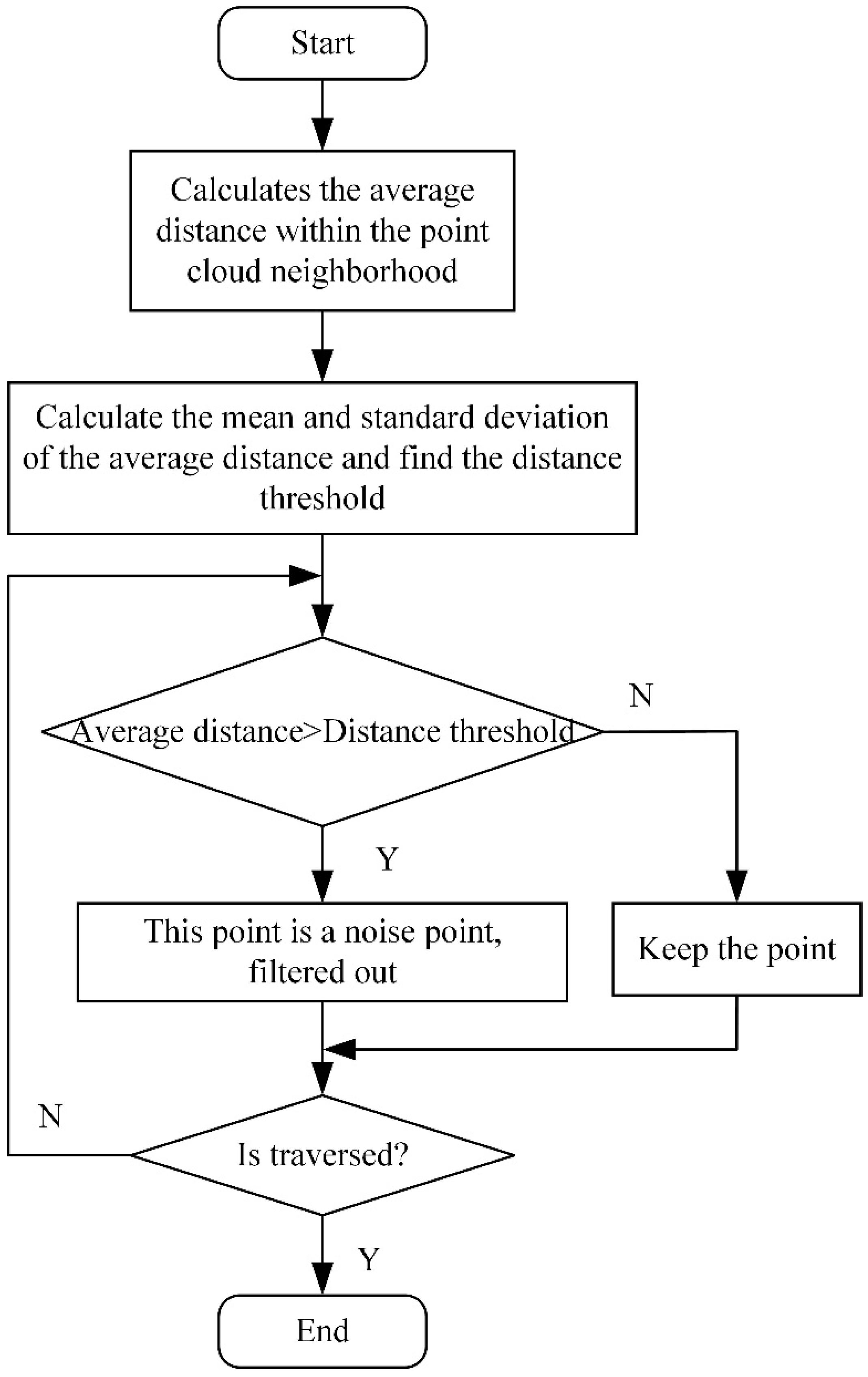
Figure 1. Flowchart of statistical filter.
Wevj 13 00130 g001
Figure 2. Removal of noise points by statistical filter: (a) original point cloud and (b) after removal of noise points.
Wevj 13 00130 g002
Figure 3. Filtering point clouds with voxel grid filter: (a) original point cloud, (b) voxel edge length of 0.2, and (c) voxel edge length of 0.3.
Wevj 13 00130 g003
Figure 4. Schematic diagram of radar longitudinal section.
Wevj 13 00130 g004
Figure 5. Ground segmentation results: (a) original point cloud, (b) RANSAC algorithm, and (c) proposed method.
Wevj 13 00130 g005
Figure 6. Grid model.
Wevj 13 00130 g006
Figure 7. Eight neighborhood grid extended clustering diagram.
Wevj 13 00130 g007
Figure 8. Boundary-box fitting process.
Wevj 13 00130 g008
Figure 9. Three-dimensional bounding box rendering.
Wevj 13 00130 g009
Figure 10. Point cloud preprocessing experiment: (a) raw point cloud, (b) point cloud filtering, and (c) ground division.
Wevj 13 00130 g010
Figure 11. Comparison of point cloud clustering results of obstacles near intelligent vehicles: (a) traditional DBSCAN algorithm and (b) the improved method proposed.
Wevj 13 00130 g011
Figure 12. Comparison of clustering results of distant obstacle point cloud of intelligent vehicle: (a) traditional DBSCAN algorithm and (b) the improved method proposed.
Wevj 13 00130 g012
Publisher’s Note: MDPI stays neutral with regard to jurisdictional claims in published maps and institutional affiliations.