Abstract
This article focuses on the trajectory tracking problem in the actuation control section of autonomous vehicles. Based on a two-degrees-of-freedom dynamics model, this paper combines adaptive preview control with a second-order sliding mode control method to develop a new control method. By designing an objective function based on lateral deviations, road boundaries, and the corresponding characteristics of the overall vehicle motion, the method adaptively adjusts the preview time to obtain the ideal yaw rate and then uses a second-order sliding mode control algorithm named Super-Twisting to calculate the steering wheel angle. Combining the low-pass filter with this controller can effectively suppress the chattering caused by the switching of the sliding mode plane while proposing a concept of smoothing based on gradient derivative, the smoothness after filtering is one-seventeenth of that before filtering, whereas the phase plane is used to prove its effectiveness and stability, it can be seen from the phase diagrams that all the state points are in the stable region. A joint simulation model of Matlab/Simulink and Carsim was built to verify the control effectiveness of the controller under the double-shift road, and the simulation results show that the designed controller has good control effect and high tracking accuracy. Meanwhile, the simulation model is also used for other simulations, firstly, simulation comparison tests were carried out with the Model Predictive Control algorithm at speeds of 36 and 54 km/h, compared to the MPC controller, the tacking accuracy of the ST controller has improved to 64.42% and 51.02% at 36 and 54 km/h; secondly, taking simulation of the designed controller against a conventional sliding mode controller based on isokinetic law of convergence, compared to the CSMC controller, the tracking accuracy of the ST controller has improved 41.78% at 54 km/h, and the smoothness of the ST controller is one-nineteenth of that of the CSMC controller; thirdly, carrying out simulations on parameter uncertainties, and replacing parameter uncertainty with Gaussian white noise, the maximum tracking error at 36 and 54 km/h did not exceed 0.3 m, and tracking remains good. Small fluctuations in the steering wheel angle do not affect the normal actuation of the actuator.
1. Introduction
Human society has developed at a rapid pace after the three industrial revolutions, and all industries are starting to move into automation and intelligence. The ultimate goal of the autonomous car, which carries mankind’s vision of the world of tomorrow, was born. It is the quintessence of the wisdom of many fields of technology, integrating environmental awareness technology, planning and decision technology, and control and execution technology, and it is a masterpiece of interdisciplinary integration. The technology of trajectory tracking is a critical aspect of control execution technology, and it relies on the underlying vehicle control technology to provide good tracking of the planned trajectory by controlling the steering wheel angle and throttle brakes; the better the control, the higher the tracking accuracy. For the time being, there are still significant safety and control concerns for self-driving cars due to imperfections in hardware and software, and good tracking accuracy is a key step in addressing this issue. Autonomous vehicles will not only reduce the probability of traffic accidents due to driver negligence, but also reduce the dependence on the vehicle for the driver’s operation, freeing up some or even of all the driver’s hands and feet, and even reaching the fifth level of autonomous vehicle [1].
Lateral control of the vehicle can be divided into preview-type and non-preview-type motion control according to different sensors. The non-predictive transverse dynamics model uses magnetic sensors to extract the transverse position of the path at the current point in relation to the desired form. This method is known as “Absolute Positioning”, it is highly adaptable to the environment but is more costly and less variable [2,3]. The preview theory actually simulates the driver’s observation of the road and the actual operation, when the driver drives, they will perform steering, acceleration, and deceleration operations to control the forward direction and driving speed of the vehicle according to the road information at a certain distance ahead and after their own experience, through these operations to ensure that it follows the expected trajectory [4]. Therefore, the application of preview control imitates the driver driving flexibly by sensing the change in curvature of the road ahead in advance.
Much modern control and non-linear control methods have been proposed by domestic and foreign researchers for the control of non-preview and preview systems based on transverse dynamics, respectively. The main methods commonly used are PID control methods [5], optimal preview control methods [6], sliding mode control methods [7,8], model predictive control methods (MPC) [9,10,11], fuzzy control methods [12], second-order sliding mode control methods [13,14], metaheuristic optimization algorithms based on swarm intelligence [15], etc. There are also intelligent optimization algorithms. In the literature [16], a novel Hammerstein model-based MPC controller has been proposed for trajectory tracking for drones. In the literature [17], this study performs the optimum path planning and tracking using the Harris hawk optimization (HHO)-grey wolf optimization algorithm, and it allows the drone to plan an optimal path and then perform good tracking. This hybrid algorithm not only avoids minimal values but also allows for faster convergence. Second-order sliding mode control improves the robustness of the system. In the literature [18], a second-order sliding mode controller based on Super-Twisting that improves the robustness and control accuracy of the underwater vehicle motion, coping with external disturbances and system uncertainties, has been designed. In the literature [19], for the trajectory tracking problem of autonomous vehicles, an adaptive super-twisting algorithm is designed to improve the robustness of the system and suppress the chattering phenomenon generated during the sliding mode.
Current research only considers preview control or second-order sliding mode control alone. This article investigates how adaptive preview control can be combined with a second-order sliding-mode control algorithm, not only to retain the benefits of adaptive preview that takes in three factors, but also to improve robustness by exploiting the properties of Super-Twisting. Firstly, the preview control takes into account the lateral deviation, road boundary and vehicle motion steering characteristics to adapt to the preview time, after which the ideal yaw rate is obtained and the difference between the ideal yaw rate and the actual yaw rate is used as the input of the sliding mode controller. Secondly, the sliding mode controller is based on Super-Twisting, which reduces chattering and improves tracking accuracy. Then, the low-pass filter is used to further attenuate the chattering of the system input.
2. Construction of the Vehicle Dynamics Model
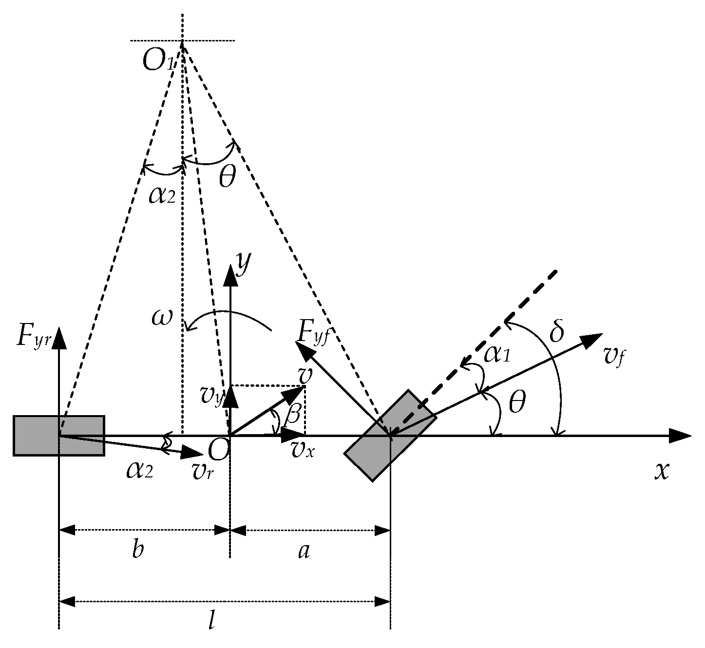
The vehicle dynamics model can be used to research handling stability, as well as ride smoothness. To facilitate the subsequent stability control analysis, a two-degrees-of-freedom dynamics model was developed and simplified to a bicycle model based on the following assumptions: (1) Ignore the effects of friction and damping in the steering system and assume that the left and right side tires have the same steering angle and speed at any given moment, taking the left and right wheel angles as inputs; (2) assume that the movement and steering of the vehicle is driven by the front wheels; (3) assume that the body and suspension system are rigid systems; and (4) ignore the transfer of front and rear axle loads. The model is shown in Figure 1 [20].

Figure 1.
Two-degrees-of-freedom vehicle dynamics model.
In Figure 1, a is the distance from the center of mass to the front axis, b is the distance from the center of mass to the rear axis, Fyf is the lateral force of the front wheel, Fyr is the lateral force of the rear wheel, vx is the longitudinal velocity, vy is the transverse velocity, ω is the angular velocity of the transverse pendulum, β is the lateral deflection of the center of mass, vf is the front wheel speed, vr is the rear wheel speed.
Assuming that the tire performance is in the linear region at small turning angles, the relationship between lateral deflection force, lateral deflection angle, and lateral deflection stiffness is as follows:
where are the front wheel lateral deflection stiffness and rear wheel lateral deflection stiffness respectively, and are front wheel lateral deflection angle and rear wheel lateral deflection angle. The front wheel side deflection angle and the rear wheel side deflection angle of the vehicle are related to its motion parameters. Assuming that the velocities of the front and rear axles of the vehicle are and respectively, the lateral deflection angle of the center of mass is ,.
Assuming that the front wheels of the car rotate at a small angle, establish the equations for the vehicle’s center of mass dynamics as follows:
where m is the mass of the whole vehicle, Iz is the rotational inertia of the vehicle at the center of mass, is the lateral acceleration, and is the angular acceleration of the transverse pendulum.
From Figure 1, the lateral deflection angles of the front and rear wheels of the car can be expressed as:
The model equations for the two degrees of freedom of the vehicle with respect to the transverse pendulum angle ω and the lateral declination angle β of the center of mass can be obtained by combining Equations (1)–(3):
3. Adaptive Preview Model
3.1. Optimum Curvature Single Point Preview
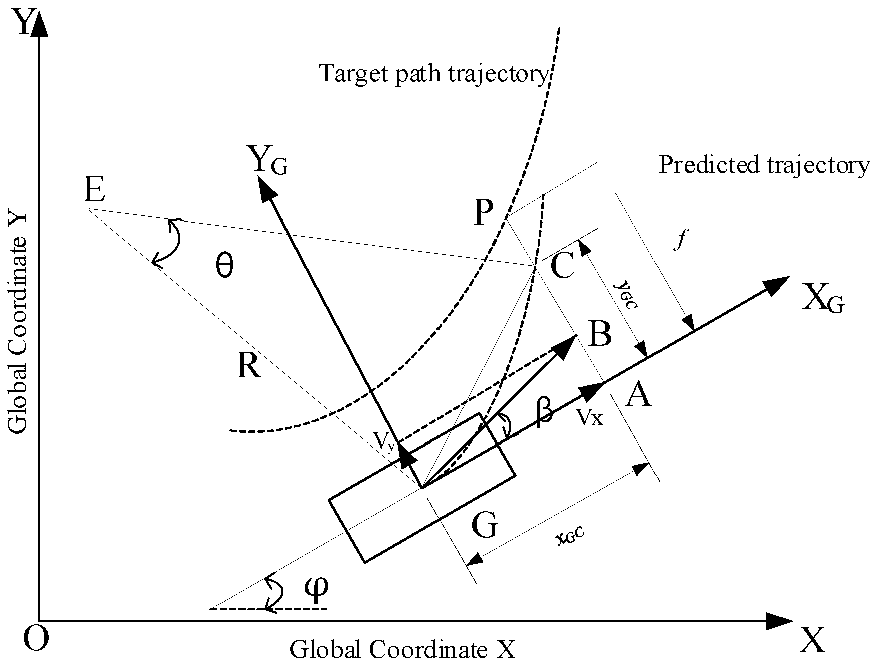
This article uses an expectation-based approach to determine the ideal steering wheel angle [21]; this method requires the assumption of a constant angular velocity of the transverse pendulum, as shown in the diagram, with the predicted trajectory treated as a circle of radius R with point E as the center and the angle of the center as θ [20]:
In Figure 2, XOY is inertial coordinate system; XG-YG is body coordinate system; point G is the position of the center of mass of the vehicle; point C is the predicted position after tp time; point P is the preview point on the target trajectory; Δf is the lateral deviation; xGC and yGC are the displacements in the XG and YG directions after tp time; φ is the vehicle heading angle; β is the mass lateral deviation angle; and v is the vehicle travel speed.
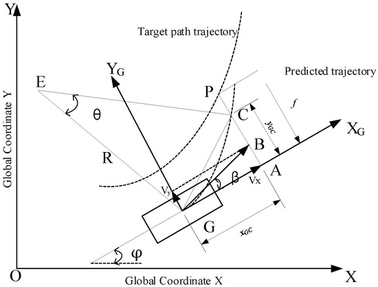
Figure 2.
Steady-state transverse pendulum angular velocity with single point preview model.
The angular velocity of the ideal transverse pendulum can be obtained as:
Parameter is calculated under the assumption of steady-state transverse pendulum angular velocity, so there is a slight deviation from the theoretical one. During the simulation, it was found that the magnitude of is related to the velocity, and after extensive simulation verification, the formula for calculating was adjusted as follows:
3.2. Adaptive Preview Time
It imitates the driver’s ability to get a flexible preview distance according to different road conditions by selecting different preview times tp, generally in the range of 0.3 to 1.5 s.
L_Drv_2 is the lateral offset between the current centroid and the actual trajectory, and the cost function designed according to L_Drv_2 is as follows [20]:
where L_Drv_2 is the lateral offset, t is model prediction time.
In order to ensure that the car can safely cross the road and satisfy the boundary constraints, the optimization function based on the distance between the trajectory speech boundary locations can be designed as follows:
where g is security function, the closer the vehicle position is to the boundary, the larger the g value. , L_Drv_2 is the lateral offset, the width of the road is set at 3.5 m.
Limited by mechanical construction, it is also necessary to consider the dynamic response time characteristics of the steering motion of the vehicle:
where T is time associated with vehicle steering response characteristics, it can be taken as 1 s or shorter when the speed is high, and can be increased when the speed is low.
Combining the three optimization functions above, the final optimization function is obtained as follows:
where is weight factor, the setting of weights is related to the purpose achieved, is related to the accuracy of trajectory tracking; is related to the distance between the vehicle and the road boundary; is related to the response characteristics of the whole vehicle.
This study has designed a multiple criteria optimization with three selection principles to select the best preview time. The method the study used is an iterative method that through the array [0.3, 1.5] with a step size of 0.01 s, to find the smallest J at each moment (). In this study, a multi-criteria optimization method is designed that takes into account all three factors, in the simulation solution, the smallest J is found from 0.3 to 1.5 by an exhaustive iteration method with a step size of 0.01 s. The range of the three weights is 0 to 1 and the sum of the three is 1, and after extensive simulations, the parameters were finally adjusted to = 0.2, = 0.05, = 0.75.
4. Design of a Second Order Sliding Mode Controller
By combining adaptive preview and sliding mode control algorithms, a sliding mode controller based on the adaptive preview is designed, which is able to combine the advantages of both. It reflects the driver’s operating characteristics, simulates the driver’s preview time, also reflects the boundary constraint, and also reflects the motion response characteristics of the whole vehicle, and the controller is insensitive to the perturbation of parameter changes, anti-interference ability, and robustness, in order to guarantee the stability of the steering wheel rotation, improve the tracking effect of the trajectory tracking control algorithm and enhance the accuracy of the tracking controller.
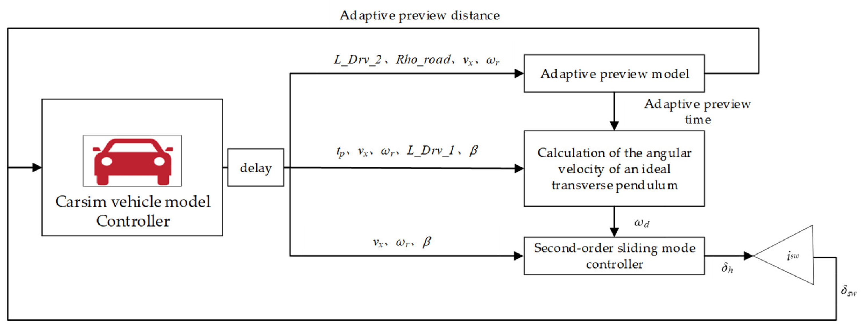
The combination of a sliding mode control method with a filter enables the control input signal to be filtered out of the chattering signal, resulting in a smooth steering wheel corner curve. The structure of the low-pass filter-based sliding mode controller control system is shown in Figure 3.
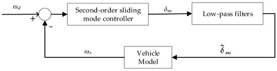
Figure 3.
Low-pass filter-based second-order sliding mode controller architecture.
4.1. Design of Low-Pass Filters
The design of the low-pass filter is shown below:
As can be seen from Figure 3:
where is the steering wheel angle and the input to the low-pass filter, is the filtered steering wheel angle and the output of the low-pass filter. is the cut-off frequency of the low-pass filter.
4.2. Design of the Super-Twisting Controller
For a system that is uncertain and requires consideration of the uptake of internal parameters as well as external disturbances, the system equation of state can be better expressed as:
Equation (4) can be rewritten according to Equation (13) as:
where , .
The equation of the controlled system can be expressed as the following equation of the state:
The uncertainty of the system and imposed disturbances are expressed in terms of , which can be expressed as:
Taking Equation (18) into Equation (17), we obtain:
The difference between the actual transverse pendulum angular velocity ωr and the ideal transverse pendulum angular velocity ωd is chosen as the tracking error of this system:
The switching function is selected as follows:
where is a positive integer.
Taking Equation (20) into Equation (21) and the derivative of Equation (21), we obtain:
In the research of second-order sliding mode control, the control input directly affects the sign and amplitude of s, and in general, it is possible to find a switching logic that is related to s and s and which ensures that the state of the system converges to in finite time. Super-Twisting is the most commonly used of the second-order sliding mode control methods, which occurs because of its advantages: (1) Its controller structure is simple and requires little information, it only needs information about the sliding mode variable s and no other information; (2) it can be applied directly if the relative order of the system with respect to s is 1; and (3) convergence is fast and the system chattering is little [22,23].
The algorithm for Super-Twisting is as follows:
Theorem 1.
Consider a class of systems satisfying Equation (23), when k1 > 0, k2 > 0, the system state can converge steadily in finite time and reach the origin point (0,0). At this time, .
Proof of Theorem 1.
Let , because k1 > 0, k2 > 0, then matrix is the Hurwitz. For any positive definite matrix P that satisfies the Lyapunov equation:
Defining the Lyapunov function , is a continuous positive definite function, and everywhere but {s = 0} is differentiable. Therefore, the chain rule can be used to derive it:
Derivation of Equation (25), we can get:
For , we can get:
where , , .
Derivative for V0, we can get:
So, when , , then can converge steadily to 0 in finite time. And system Equation (23) can converge steadily to 0 in finite time and Theorem 1 can be proved. □
From Equations (22) and (23), when the system is steady, , we can get:
Then, we can get:
In order to obtain the final control quantity, the equation for calculating the angle from the front wheel to the steering wheel is as follows:
where isw is the angular transmission ratio of the steering wheel angle and the wheel angle.
The following Table 1 shows the relevant parameters for the ST algorithm.

Table 1.
Parameters of ST controller.
4.3. Phase Diagram Analysis of the Vehicle Dynamic Stability
The phase plane method is based on the time domain to analyze the dynamics within each system and illustrates the dynamic information of the system graphically by plotting the interrelationships of the states within the system.
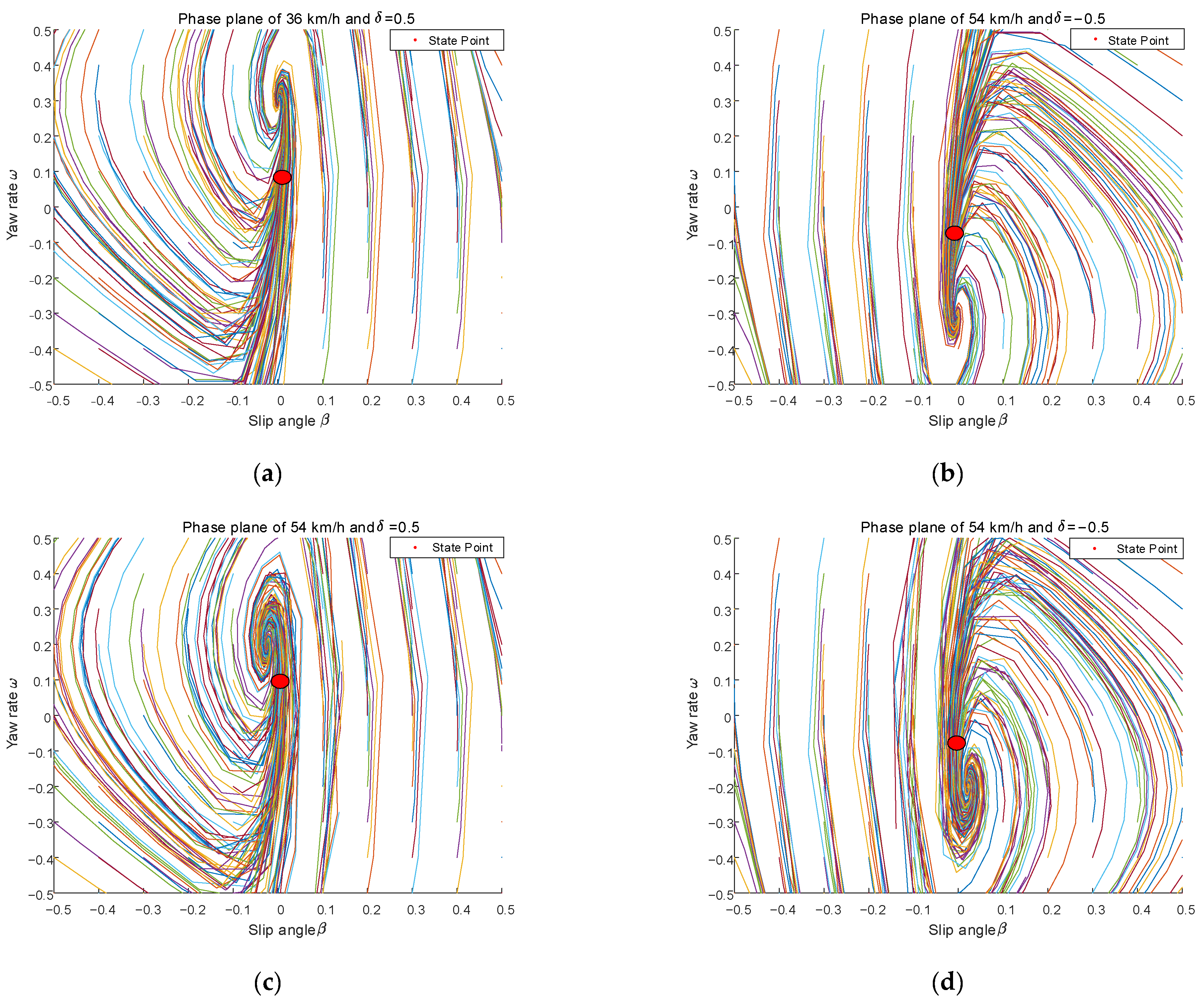
At a speed of 36 km/h, the front wheel angles are set to 0.5 and −0.5 rad to find the front wheel angle δ and yaw rate ω at the corresponding moments, and the following phase diagram can be derived from the two-degree-of-freedom dynamics model; similarly, at a speed of 54 km/h, the front wheel angles are set to 0.5 and −0.5 to find δ and ω at the corresponding moments, and the following phase diagram can be derived (where δ and ω are represented by the State Point).
The ranges of initial values for both β and ω is [−0.5, 0.5], the step for both β and ω is 0.1. By setting different initial values, different colored lines in Figure 4 can be obtained by substituting them into the two degrees of freedom dynamics model. This means that different colored lines represent the relationship between β and ω at different initial values of β and ω. From Figure 4, the vortex line will converge to the center gradually with the change of motion. This suggests that the region of these whirlpool lines is stable, and the state points taken from the trajectory are all on the line that can converge to the center, and it can be seen that each state point corresponding to the front wheel corner is located near the equilibrium point and tends to move toward the equilibrium point, so the controller is designed to be stable.
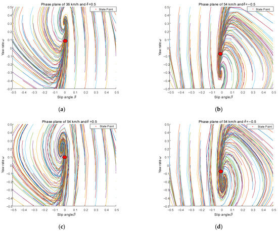
Figure 4.
Phase plane at different speeds and front wheel angles. (a) Phase plane of 36 km/h and δ = 0.5 rad; (b) phase plane of 36 km/h and δ = −0.5 rad; (c) phase plane of 54 km/h and δ = 0.5 rad; (d) phase plane of 54 km/h and δ = −0.5 rad.
4.4. Low-Pass Filter Validation
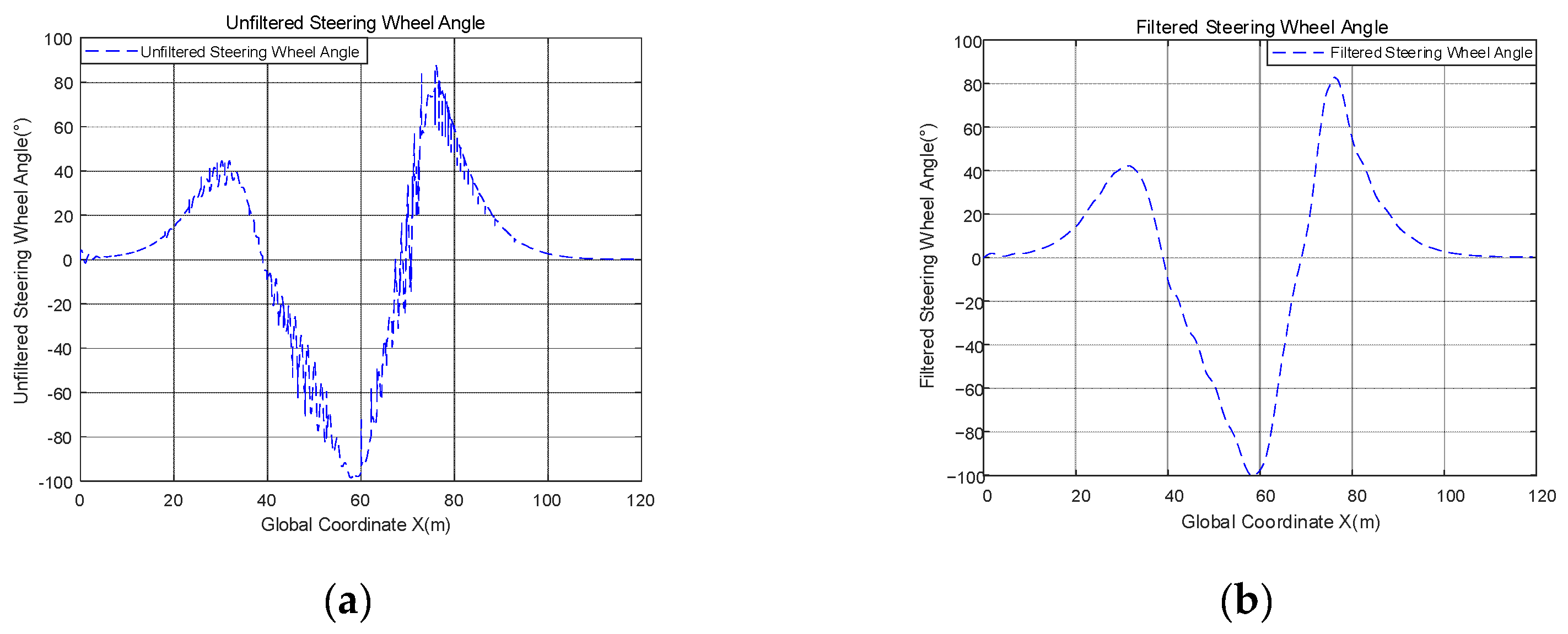
To test the effectiveness of the low-pass filter, a comparative test was conducted. The road adhesion coefficient was set as 0.7 and the speed was set as 54 km/h. The steering wheel angles before and after filtering are shown as Figure 5.
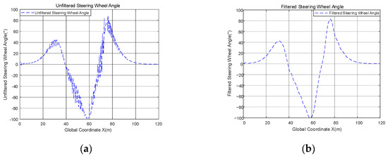
Figure 5.
Steering wheel angle before and after filtering. (a) Unfiltered steering wheel Angle; (b) filtered steering wheel angle.
The smoothness of the curve is evaluated using the method of finding the derivative of the discrete points using the gradient, which uses the method of centroid differencing, the gradient reflects the rate of change of the value. The unfiltered steering wheel corner discrete point array is noted as steer0, the filtered steering wheel corner discrete point array is noted as steer1, and the smoothness evaluation function of the curve takes the form of the standard deviation of the gradient, as follows:
where F is the one-dimensional value of the steering wheel angle, gradient is the gradient function, Fdx is the gradient of the steering wheel angle, S is the standard deviation, of the gradient and defines S as smoothness, μ is the mean of the gradient.
After simulation, the smoothness of the unfiltered steering wheel angle Ssteer0 = 0.7107, and the smoothness of the unfiltered steering wheel angle Ssteer1 = 0.0418. The range of the gradient of unfiltered angles is [−13.8526, 13.2884], the average of it is 7.9913 × 10⁻⁶; the range of the gradient of filtered angles is [−0.1192, 0.1825], the average of it is 1.1592 × 10⁻⁵. As can be seen from these values, the mean values of the gradients before and after filtering are approximately equal, however, the maximum value of the gradient before filtering is 72.8131 times greater than after filtering, and the gradient reflects the rate of change of the value. This means that the value of the steering wheel angle before filtering varies quite sharply compared to after filtering, and a large value of the gradient indicates the presence of a large jitter in the curve, and this shows the smoother curve of the steering wheel corner after filtering. Also, Ssteer0 is 17.0024 times larger than Ssteer1, and this means that the gradient of the filtered angle is much less discrete than before filtering, and the gradient values of the filtered angle are closer to the average. In summary, it can be concluded that the low-pass filter works well and the filtered curve is smoother.
5. Design of the MPC Controller
The basic idea of model predictive control is to use the existing model, the current state of the system, and the future control quantity to predict the future output of the system, and to achieve the control purpose by solving the constrained optimization problem on a rolling basis, with three features: predictive model, rolling optimization and feedback correction. Model predictive control is based on time series for rolling optimization, and solves the corresponding control time domain in the prediction time domain [24,25].
5.1. MPC Output Function Derivation
The MPC algorithm uses an error model under a kinematic model with the following state space equations for the kinematic model:
Notate , taking into Equation (34), and using the Taylor series expansion and ignoring higher order terms gives:
The error model can be obtained:
Define the output equation:
where , C is a constant.
The output equation can be derived:
where , .
5.2. MPC Algorithm Objective Function Design
Defining the reference values of the system output quantities:
Subtract Equation (39) from Equation (38) gives:
Defining Equation (40) becomes as follows:
The design objective function is:
Defining , taking and into Equation (42) we can obtain:
Defining , , Equation (43) can be transformed as follows:
5.3. MPC Algorithm Constraint Design
Constraints are designed to constrain control quantities and control increments, such as speed and front wheel angle. The constraints are designed as follows:
The control volume constraint sum as follows:
Control of incremental constraints as follows:
The objective function can be designed as:
where is a relaxation factor to prevent no solution when calculating the optimal solution.
5.4. MPC Simulation Verification
First set the control volume and control increments:
The other parameters in the MPC algorithm are shown in Table 2.
Table 2.
Parameters of MPC algorithm.
6. Design of the Conventional Sliding Mode Control (CSMC) Controller
This subsection shows a CSMC controller based on the isokinetic law of convergence [22]. The general form of the isokinetic law of convergence is as follows:
From Equations (22) and (51), the control input of this conventional SMC can be obtained:
Choosing a Lyapunov function candidate and differentiating V with respect to time, we have:
Taking Equation (52) into Equation (53), when , , we have:
The control system is convergent and can converge to 0 in finite time.
7. Control System Simulation Verification
7.1. Construction of a Joint Simulation Platform
The vehicle data from Carsim is sent to the model built in Simulink as an S-function, and the designed second-order sliding mode controller is added to the model, as shown in Figure 6.
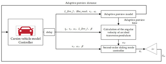
Figure 6.
Combined Carsim-Simulink simulation model.
This is followed by setting the input and output parameters of Carsim, the first two being the inputs and the others being the outputs, as shown in Table 3.
Table 3.
Parameters for Carsim input and output.
7.2. ST Controller Simulation without Considering the Uncertainty of the Parameters
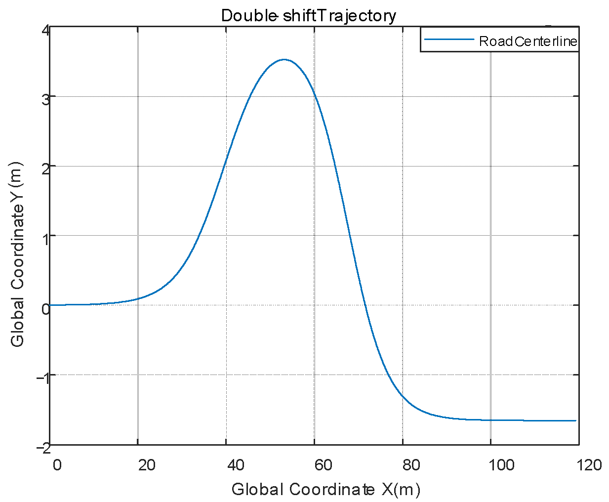
Using the same double-shifted trajectory of Equation (55), the double-shifted path was set up in Carsim, adding all trajectory points in the form of discrete points according to their X and Y coordinates, followed by a simulation verification step. The selected working condition is a double-shift line, and the following equation is used as the double-shift line trajectory, as the ideal trajectory:
where , , , .
The double-shifted road is shown in Figure 7.
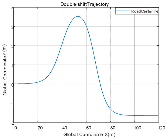
Figure 7.
Double shift road diagram.
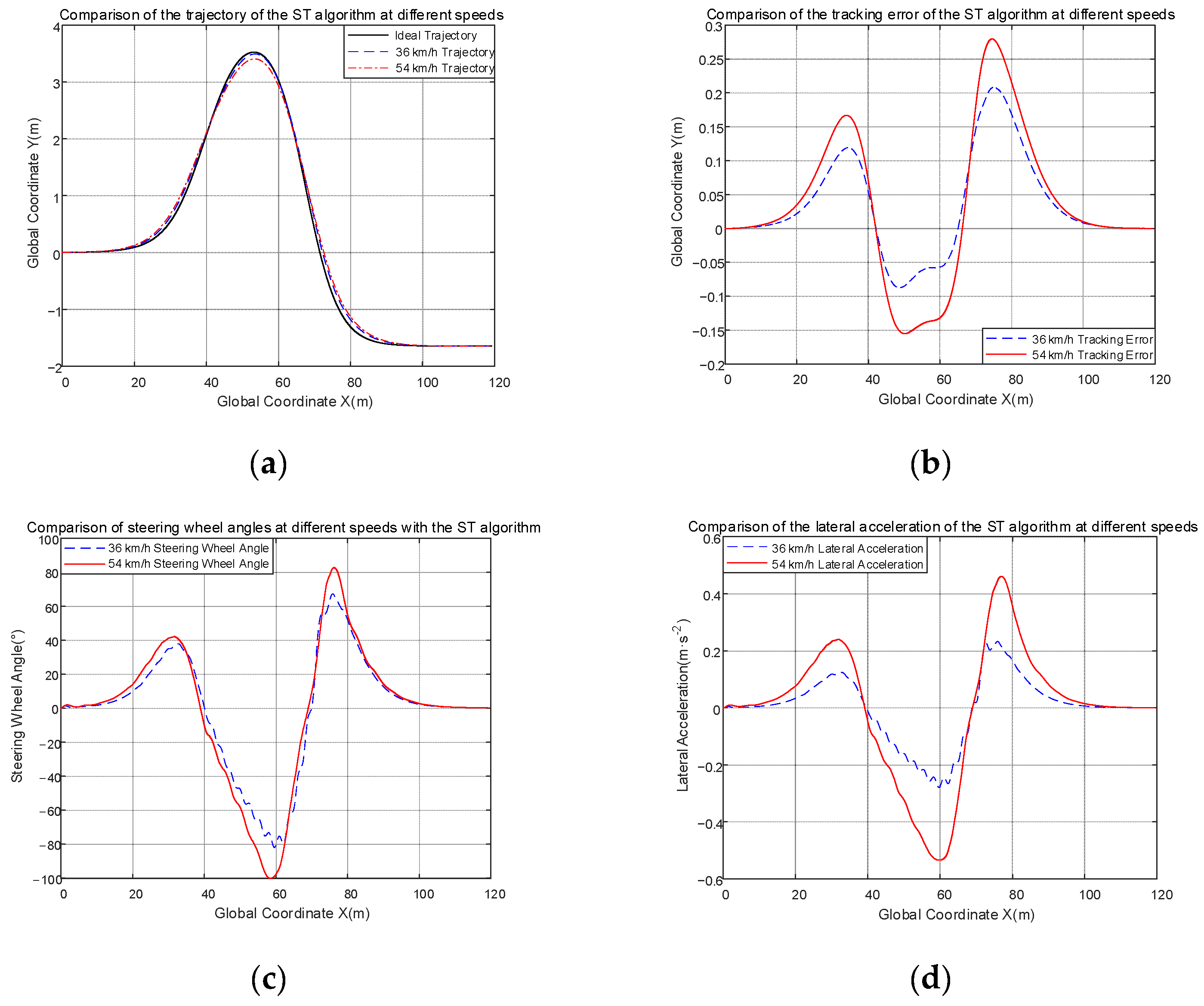
This simulation does not take into account the uncertainly of the parameters, and for this reason E(t) is set to 0. The road surface coefficient was set to μ = 0.7, and the car was allowed to track the set double-shifted line path at longitudinal speeds of 36 and 54 km/h, respectively. Taking the lateral offset from the vehicle center of mass to the road centerline as the tracking error, the joint simulation results for different speeds are compared for each parameter as follows.
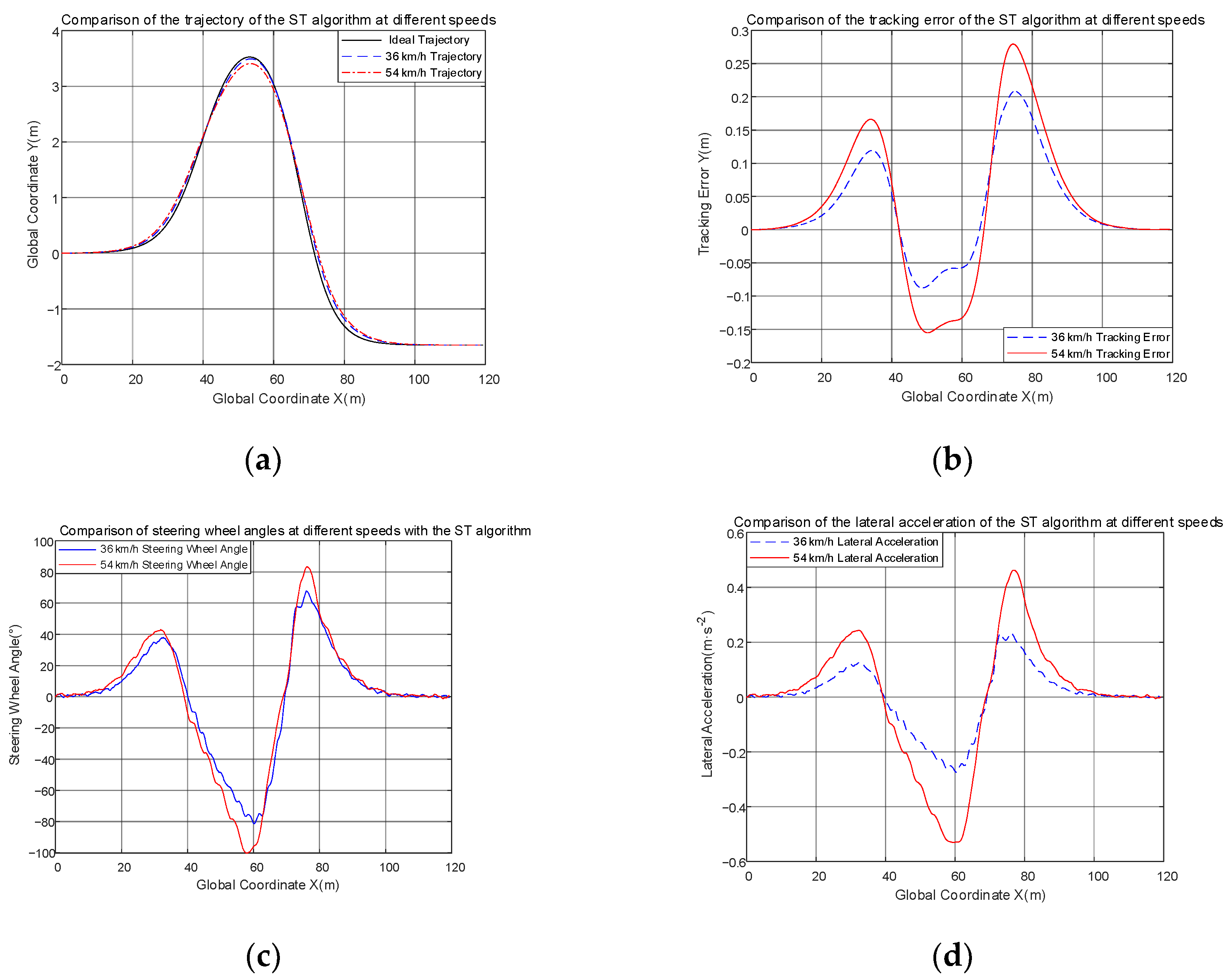
As can be seen from Figure 8, in the double-shifted line condition, the controller designed in this paper has a good control effect and the actual trajectory basically matches the ideal trajectory curve in Figure 8a—the slower the speed, the better the fit of the track. In Figure 8b, the range of tracking error at 36 km/h is [0.2082, −0.0874] and the range of tracking error at 54 km/h is [−0.1553, 0.2795]. It can be seen that the range of tracking error increases with speed. The distance from the center line of the road to the road boundary is 1.75 m, and the maximum deviation of the vehicle’s trajectory does not exceed 0.3 m. So, the designed controller tracks well. In Figure 8c, the smoothness of the steering wheel angle at 36 km/h is 0.0287, at 54 km/h is 0.0418, and the range of the gradient value of the angle at 36 km/h is [−0.0694, 0.1778], at 54 km/h is [−0.1192, 0.1825], the average of the gradient value at two speeds is 0. These data mean the dispersion of the angles is small and the values are very close to 0, and there is no violent chattering. In this figure, small fluctuations in the curve are caused by the slip mode controller’s own slip mode surface switching, and the limitations of the low-pass filter’s filtering effect. The curve is already very smooth compared to the pre-filtering curve. In Figure 8c,d, at X = 60 m and X = 80 m, the curves both show slight fluctuations due to the fact that at both locations the curvature of the road, also known as the curvature of the road, is greater and requires larger corners. In general, the overall control of the designed ST controller is good.
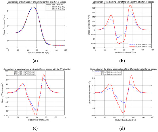
Figure 8.
Comparison of different parameters at different speeds. (a) Comparison of trajectories at different speeds; (b) comparison of tracking error at different speeds; (c) comparison of steering angle at different speeds; (d) comparison of lateral acceleration at different speeds.
7.3. Comparison Tests of ST Controller and MPC Controller
If you set the working condition as a double-shifted road, the road adhesion coefficient to 0.7, the speed to 36 and 54 km/h, and take the vehicle’s center of mass to the road centerline offset as the tracking error, the joint simulation results are in Figure 9.
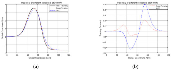
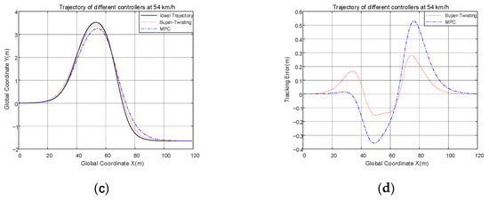
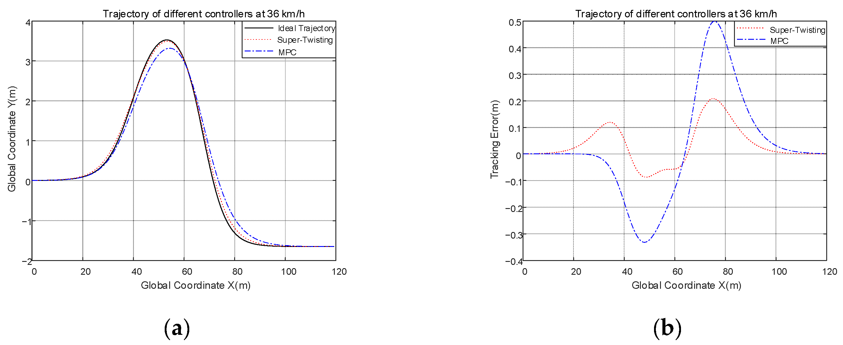
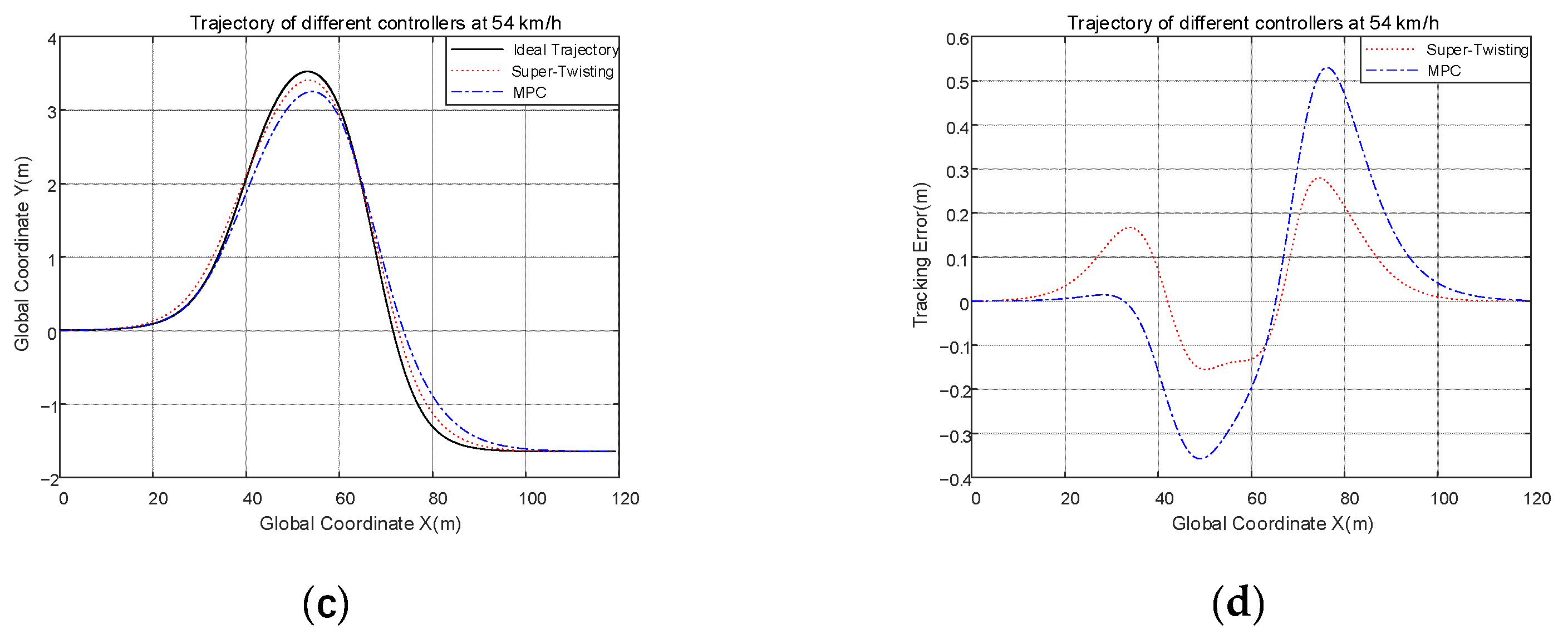
Figure 9.
(a) Comparison of trajectories at 36 km/h; (b) comparison of the tracking error at 36 km/h; (c) comparison of trajectories at 54 km/h; (d) comparison of the tracking error at 54 km/h.
As seen from Figure 9, in the two different speed conditions, the trajectory of the ST controller is more closely aligned to the ideal trajectory than the MPC controller, and the ST controller provides better control results. At 36 km/h, the range of tracking error of the ST controller is [−0.0874, 0.2082], and it defines tracking accuracy as the maximum value minus the minimum value. The tracking accuracy of the ST controller is 0.2956, the range of tracking error of the MPC controller is [−0.3314, 0.4993], and the tracking accuracy of the MPC controller is 0.8307. Compared with the CSMC controller, the control precision of the ST controller is improved by 64.42%. The tracking error can directly represent the tracking impact of the controller, and it is apparent that the tracking error of the ST controller is smaller, and the effect of tracking of the ST is better. At 54 km/h, the range of tracking error of the ST controller is [−0.1553, 0.2795], the tracking accuracy of the ST controller is 0.4348, and the range of tracking error of the MPC controller is [−0.3580, 0.5297], the tracking accuracy of the MPC controller is 0.8877. Compared with the CSMC controller, the control precision of the ST controller is improved by 51.02%. It follows then that the tracking error of the ST controller is smaller, and the effect of the tracking of the ST is better.
7.4. Comparison Tests of ST Controller and CSMC Controller
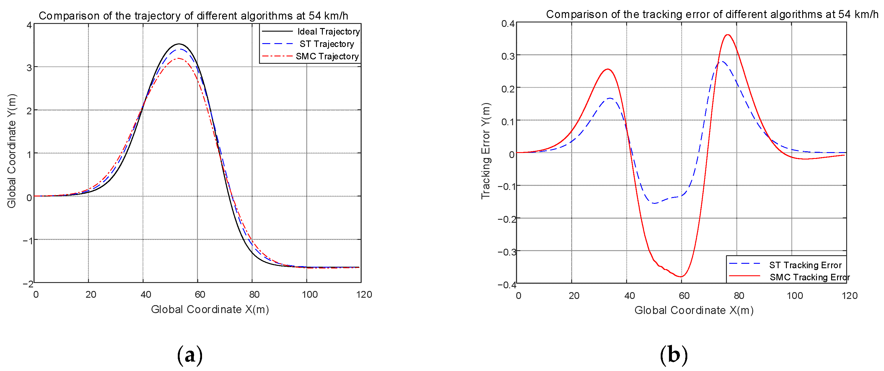
If you set the working condition as a double-shifted road, the road adhesion coefficient to 0.7, the speed to 54 km/h, and take the vehicle’s center of mass to the road centerline offset as the tracking error, the joint simulation results are as follows:
As shown in Figure 10a, it is clear to see that the trajectory of the ST controller is more closely aligned with the ideal trajectory, and this can be proved in Figure 10b. The range of tracking error of the ST controller is [−0.1553, 0.2795], which defines tracking accuracy as the maximum value minus the minimum value, and the tracking accuracy of the ST controller is 0.4348; the range of tracking error of the CSMC controller is [−0.3803, 0.3614], the tracking accuracy of the CSMC controller is 0.7417. Compared with the CSMC controller, the control precision of the ST controller is improved by 41.78%. In contrast with the different range of different controllers, this proves the superiority of the ST controller in terms of control effect.
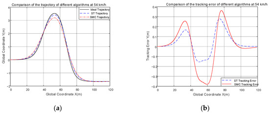
Figure 10.
(a) Comparison of trajectories at 54 km/h; (b) comparison of the tracking error at 54 km/h.
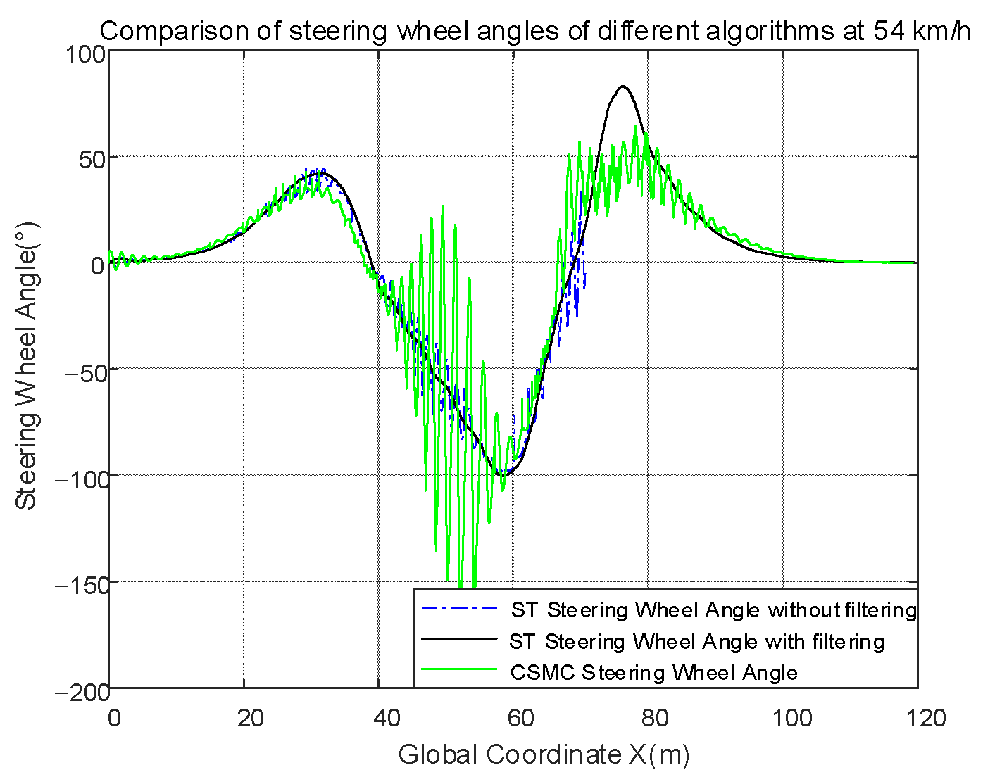
The input of the ST controller and the CSMC controller is the steering wheel angle, and the ST controller adopts a low-pass filter to keep buffeting. The steering wheel angle of the three cases is as follows.
The disadvantages of sliding mode control can be seen visually in Figure 11, i.e., it leads to high-amplitude and high-frequency chattering in the control input. Using the previously designed smoothness Equation (32), we can obtain the smoothness of the three conditions: the smoothness of steering wheel angle of the ST controller with unfiltered (STUF) is SSTUF = 0.7107, the smoothness of steering wheel angle of the CSMC controller is SCSMC = 0.7990, the smoothness of steering wheel angle of the ST controller with filtering (STF) is SSTF = 0.0418. In numerical terms, SSTUF is 17.00 times larger than SSTF, SCSMC is 19.11 times larger than SSTF, which shows the smooth curve of the angle compared to the other two. The range of the gradient of unfiltered angles of the STUF controller is [−13.8526, 13.2884], the range of the CSMC controller is [−7.8851, 11.8837], and the range of the STF controller is [−0.1192, 0.1825]. The gradient reflects the rate of change of the value, therefore, in terms of the range of the gradient, the variation range of the angles of the STUF controller is smaller than that of the CSMC controller, while that of STF controller is smaller than that of STUF controller. This indicates that the STF controller has a smoother angular profile with less undulation and less chatter than the other two. The average gradient of angles of STUF is 7.9913 × 10⁻⁶, the average of angles of CSMC is −8.1337 × 10⁻⁶, and the average of angles of STF is 1.1592 × 10⁻⁵. Numerically, the values of all three averages are close to 0, the smoothness reflects the degree of dispersion of the gradient, and consequently, the degree of dispersion of STF is the smallest of the three. This further illustrates that the filtered ST controller produces only a litter chattering compared to the other two.
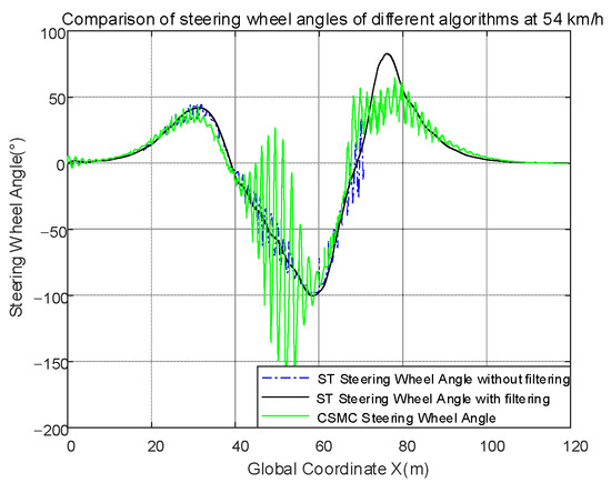
Figure 11.
Comparison of steering wheel angles of different algorithms at 54 km/h.
7.5. Simulation with Considering the Uncertainty of the Parameters
The road setting and road conditions are the same as before. Considering the method in Book [26], in Equation (18), considering the system perturbation, take , , , , as a result, . Then this simulation uses the Band-Limited White Noise block in Matlab/Simulink to represent uncertainty, i.e., disturbances external to and internal to the system. Set sample time = 0.01, noise power = 0.2 × 0.2 × 0.01, and this setting indicates an amplitude of 0.2 and a sampling frequency of 100 Hz. The white noise of the setup is shown in Figure 12.
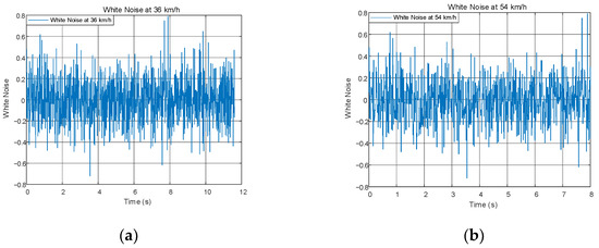
Figure 12.
(a) Comparison of trajectories at 36 km/h; (b) comparison of tracking error at 54 km/h.
The comparisons of simulations with different speeds in the presence of uncertainty are shown in Figure 13.
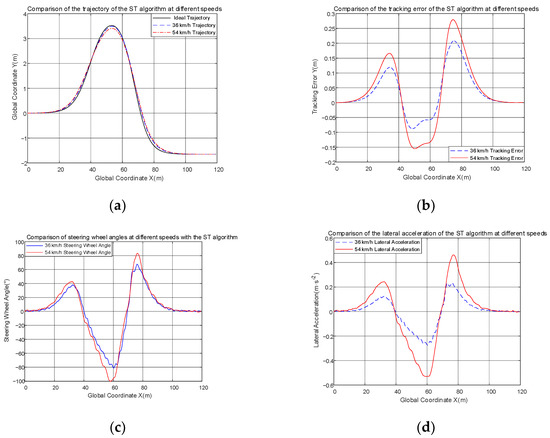
Figure 13.
(a) Comparison of trajectories at different speeds; (b) comparison of tracking error at different speeds; (c) comparison of steering angle at different speeds; (d) comparison of lateral acceleration at different speeds.
By using Gaussian white noise as a disturbance of uncertainty, it can be seen from Figure 13a that the trajectory tracking of the ST controller is still very good at both speeds and the trajectory is relatively close to the ideal trajectory. In Figure 13b, the range of tracking error of the ST controller at 36 km/h is [−0.0877, 0.2086], at 54 km/h is [−0.1552, 0.2795], and the tracking error increases as speed increases, the tracking accuracy at 36 km/h is 0.2963, the tracking accuracy at 54 km/h is 0.4347. The maximum tracking error at both speeds is not exceeding 0.3 m, this indicates good tracking. Then, in Figure 13c,d, there is some chattering in the curve, and this is due to the inclusion of the uncertain interference of Gaussian white noise, and due to the controller’s own slip-side switching, a little bit of jitter remains despite the low-pass filter to attenuate it. These remaining chattering switches are relatively small, and the switching is not drastic, therefore, the actuators can still be executed normally. In summary, the designed ST controller is still robust to uncertainties.
8. Conclusions
- This article designs a second-order sliding mode controller based on the ST algorithm, which combines an adaptive preview controller with the second-order sliding mode algorithm. The adaptive preview can take into account the trajectory deviation, road boundary, and overall vehicle motion response characteristics to solve for a suitable preview time and set a matching preview distance to make the controller more in line with the driver’s habits so that it can sense the road ahead in advance to make the corresponding control strategy. Finally, the Lyapunov function and phase plane analysis methods are used to prove its convergence and stability respectively;
- In designing the ST second-order sliding mode control algorithm, the chattering is also further reduced by combining a low-pass filter with the ST algorithm. This paper also proposes a method based on the standard deviation of the gradient to calculate the smoothness of the curve, using this parameter to evaluate the chattering of the curve, the standard deviation of the gradient was used to evaluate smoothness, and the smoothness after filtering is one-seventeenth of that before filtering;
- The ideal yaw rate can be obtained by adaptive preview control. The difference between the ideal yaw rate and the actual yaw rate is fed into the designed ST second-order sliding mode controller to solve the required steering wheel angle as the target for tracking control. To demonstrate the effectiveness of this controller, an MPC algorithm was designed for comparison experiments. Compared to the MPC controller, the tracking accuracy of the ST controller has improved to 64.42% and 51.02% at 36 and 54 km/h, respectively. At the same time, it was also compared with conventional sliding mode control and the results showed that the tracking accuracy of the ST controller has improved to 41.78%, and the smoothness of the ST controller is one-nineteenth that of the CSMC. This means the ST controller can produce inputs with weaker chattering; and
- Simulations are carried out on parameter uncertainties in this article, where parameter uncertainties include system parameter uptake and external disturbances, and Gaussian white noise is used to replace these uncertainties. With simulation at 36 and 54 km/h, the simulation results show that despite the effect of Gaussian white noise, the trajectory of the ST controller still fits the ideal trajectory and the tracking error does not exceed 0.3 m. Although there are slight fluctuations in the steering wheel angle and transverse angular velocity, they are still within the acceptable range and the actuator still works properly.
Author Contributions
Conceptualization, S.B. and H.H.; methodology, H.H.; software, H.H. and J.T.; validation, H.H.; formal analysis, H.T., B.L. and S.B.; investigation, H.H.; resources, H.H., B.L. and S.B.; data curation, H.H.; writing-original draft preparation, H.H., Y.Z., Z.Q. and H.T.; writing-review and editing, H.H., Z.Q. and B.L.; visualization, H.H.; supervision, B.L. and S.B.; project administration, B.L. and S.B.; funding acquisition, not applicable. All authors have read and agreed to the published version of the manuscript.
Funding
This research was funded by “Postgraduate Research & Practice Innovation Program of Jiangsu Province” under grant number XSJCX21_22, “the Natural Science Foundation of the Jiangsu Higher Education of China” under grant number 21KJA580001, “the National Natural Science Foundation of China” under grant number 52172367 and “the National Natural Science Foundation of China Youth Program under grant number 51705220. The APC was funded by 52172367.
Data Availability Statement
Not applicable.
Conflicts of Interest
The authors declare no conflict of interest.
References
- Hao, Y. Overview on the Research of Lateral and Longitudinal Control for Intelligent Vehicles. Automob. Appl. Technol. 2022, 47, 158–161. [Google Scholar] [CrossRef]
- Jinghua, G.; Keqiang, L.; Yugong, L. Review on the research of motion control for intelligent vehicles. J. Automot. Saf. Energy 2016, 7, 151–159. [Google Scholar]
- Wiseman, Y. Autonomous Vehicles. In Advances in Information Quality and Management; Khosrow-Pour, D.B.A.M., Ed.; IGI Global: Harrisburg, PA, USA, 2021; pp. 1–11. ISBN 978-1-79983-479-3. [Google Scholar]
- Li, W. Research on Intelligent Vehicle Path Following Control Based on Preview Distance Active Optimization. Master’s Thesis, Jiangsu University, Zhenjiang, China, 2021. [Google Scholar] [CrossRef]
- Zhang, X.; Li, J. Lateral and longitudinal coordinated control for intelligent-electricvehicle trajectory-tracking based on LQR-dual PID. J. Automot. Saf. Energy 2021, 12, 346–354. [Google Scholar]
- Li, Y.; Liu, Y.; Feng, Q.; Nan, Y.; He, J.; Fan, J. Path tracking control for an intelligent commercial vehicle based on optimal preview and model predictive. J. Automot. Saf. Energy 2020, 11, 462–469. [Google Scholar] [CrossRef]
- Sun, H. Research on Tracking Control Method of Unmanned Vehicle Based on Sliding Mode Variable Structure. Master’s Thesis, Changchun University of Technology, Changchun, China, 2021. [Google Scholar] [CrossRef]
- Li, L.; Li, J.; Zhang, S. Trajectory tracking control of autonomous vehicles with optimized sliding mode control. J. Automot. Saf. Energy 2020, 11, 503–510. [Google Scholar] [CrossRef]
- Wang, K.; Li, Q.; Wang, Z.; Yang, J. Trajectory tracking control for automated vehicle based on NMPC considering vehicle rolling motion. Control Decis. 2021, 1–8. [Google Scholar] [CrossRef]
- Wang, Q.; Mao, Z.; Zhang, D.; He, Z.; Lv, Z. Lane Changing Path Tracking Control Based on Trajectory Prediction and Model Prediction. Control Eng. 2022, 4, 1–9. [Google Scholar] [CrossRef]
- Li, C.; Wang, S.; Liu, M.; Pneg, Z.; Nie, S. Research on the Trajectory Tracking Control of Autonomous Vehicle Based on the Multi-Objective Optimization. Automob. Technol. 2022, 8–15. [Google Scholar] [CrossRef]
- Chen, Y. AGV Trajectory Tracking System Based on Adaptive Fuzzy Control. Automob. Appl. Technol. 2021, 46, 22–24. [Google Scholar] [CrossRef]
- Sun, Z.; Zheng, J.; Man, Z.; Fu, M.; Lu, R. Nested Adaptive Super-Twisting Sliding Mode Control Design for a Vehicle Steer-by-Wire System. Mech. Syst. Signal Process. 2019, 122, 658–672. [Google Scholar] [CrossRef]
- Xu, M.; Fang, Y.; Li, J.; Zhao, X. Finite time distributed coordinated control for attitude of multi-spacecraft based on super-twisting algorithm. Control Theory Appl. 2021, 38, 924–932. [Google Scholar] [CrossRef]
- Altan, A. Performance of Metaheuristic Optimization Algorithms Based on Swarm Intelligence in Attitude and Altitude Control of Unmanned Aerial Vehicle for Path Following. In Proceedings of the 4th International Symposium on Multidisciplinary Studies and Innovative Technologies, Istanbul, Turkey, 22–24 October 2020. [Google Scholar] [CrossRef]
- Altan, A.; Hacıoğlu, R. Model Predictive Control of Three-Axis Gimbal System Mounted on UAV for Real-Time Target Tracking under External Disturbances. Mech. Syst. Signal Process. 2020, 138, 106548. [Google Scholar] [CrossRef]
- Belge, E.; Altan, A.; Hacıoğlu, R. Metaheuristic Optimization-Based Path Planning and Tracking of Quadcopter for Payload Hold-Release Mission. Electronics 2022, 11, 1208. [Google Scholar] [CrossRef]
- Huang, B.; Yang, Q. Trajectory Tracking Control Method of a Work-class ROV Based on a Super-twisting Second-order Sliding Mode Controller. J. Unmanned Undersea Syst. 2021, 29, 14–22. [Google Scholar] [CrossRef]
- Ao, D.; Huang, W.; Wong, P.K.; Li, J. Robust Backstepping Super-Twisting Sliding Mode Control for Autonomous Vehicle Path Following. IEEE Access 2021, 9, 123165–123177. [Google Scholar] [CrossRef]
- Hu, H.; Bei, S.; Zhao, Q.; Han, X.; Zhou, D.; Zhou, X.; Li, B. Research on Trajectory Tracking of Sliding Mode Control Based on Adaptive Preview Time. Actuators 2022, 11, 34. [Google Scholar] [CrossRef]
- Chen, W.; Tan, D.; Wang, H.; Wang, J.; Xia, G. A Class of Driver Directional Control Model Based on Trajectory Prediction. J. Mech. Eng. 2016, 52, 106–115. [Google Scholar] [CrossRef]
- Li, P. Research and Application of Traditional and Higher-Order Sliding Mode Control. Ph.D. Thesis, National University of Defense Technology, Changsha, China, 2011. [Google Scholar]
- Cai, C. Ship Straight-path Following Control Based on High-order Slide Mode. Master’s Thesis, Dalian Maritime University, Dalian, China, 2017. [Google Scholar]
- Bai, S. Research on Intelligent Vehicle Trajectory Tracking Method Based on Model Predictive Control. Master’s Thesis, Harbin University of Science and Technology, Harbin, China, 2021. [Google Scholar] [CrossRef]
- Mohammad, R.; Navid, M.; Saeid, N.; Shady, M. Model Predictive Control with Learned Vehicle Dynamics for Autonomous Vehicle Path Tracking. IEEE Access 2021, 9, 128233–128249. [Google Scholar] [CrossRef]
- Xiao, L. Sliding Mode Control for Aerospace Power System; Zhejiang University Press: Hangzhou, China, 2018; pp. 242–256. [Google Scholar]


Publisher’s Note: MDPI stays neutral with regard to jurisdictional claims in published maps and institutional affiliations. |
© 2022 by the authors. Licensee MDPI, Basel, Switzerland. This article is an open access article distributed under the terms and conditions of the Creative Commons Attribution (CC BY) license (https://creativecommons.org/licenses/by/4.0/).