Research on Intelligent Vehicle Motion Planning Based on Pedestrian Future Trajectories

Abstract

This work proposes an improved pedestrian social force model for pedestrian trajectory prediction to prevent intelligent vehicles from colliding with pedestrians while driving on the road. In this model, the intelligent vehicle performs motion planning on the basis of predicted pedestrian trajectory results. A path is planned by using the fifth-order Bezier curve, the optimal coordinate is acquired by adjusting the weight coefficient of each optimisation goal, and the optimal driving trajectory curve is planned. In speed planning, the pedestrian collision boundary is proposed to ensure pedestrian safety. The initial speed planning is performed by a dynamic programming algorithm, and then the optimal speed curve is obtained by quadratic programming. Finally, the front pedestrian deceleration or uniform speed scene is set for simulation verification. Simulation results show that the vehicle speed reaches a maximum value of 6.39 m/s under the premise of ensuring safety and that the average speed of the intelligent vehicle is 4.6 m/s after a normal start process. The maximum and average speed values obtained with trajectory prediction indicate that the intelligent vehicle ensures pedestrian and vehicle safety as well as the intelligent vehicle’s economy.

1. Introduction

The occupancy rate of self-driving cars in cities is increasing with the development of science and technology. This increase is accompanied by the high-speed development of the core technology of artificial intelligence and high-performance computing hardware, which provides powerful processing hardware at low cost and the basis for solving serious safety problems on public roads. Self-driving cars are integrated with a wide range of technologies, including vehicle, information and communication technologies and artificial intelligence [1,2,3,4]. Pedestrians, as the main carriers on the road, exhibit casual and changeable directions as well as other characteristics. The purposeful and accurate prediction of pedestrian trajectory by self-driving cars has become an important research topic. However, the movement planning of self-driving cars on structured roads that consider pedestrian trajectory has become a major challenge [5,6,7,8,9].

In 1995, Helbing et al. proposed a social force model for studying pedestrian movement based on Newtonian dynamics to quantify the subjective motivation of pedestrians and considered other pedestrians or obstacles as forces that affect pedestrians [10]. Later, Helbing et al. proposed an improved social force model that well reflects the state of pedestrian flow in normal and emergency situations and has high adaptability and authenticity [11]. In recent years, the social force model has been gradually applied to trajectory prediction. Luber et al. presented a trajectory prediction model based on the social force model that considers the effects of interactions between pedestrians and verified its validity through comparison; however, this method has poor generalisation ability [12]. Alahi A et al. proposed obtaining social affinity features by learning their relative positions from pedestrian trajectories in a crowd [13]. Yi S et al. proposed the use of human attributes to improve crowd prediction [14]. By analysing the motion characteristics of e-bikes, Qu et al. proposed a mixed traffic flow model considering e-bikes based on a social force model [15]. Zhang et al. proposed an SFM-based pedestrian trajectory prediction method for unsignalled pedestrian crossing scenarios by combining the pedestrian walk–stop decision model [16]. Existing research focuses on purely pedestrian trajectory or purely intelligent vehicle motion planning. The interaction between pedestrians and vehicles in the combination of pedestrian trajectory prediction results to plan vehicle motion has become the focus of the current research [17].

In motion planning algorithms, curve interpolation is used to generate a fitted trajectory that satisfies constraints, such as feasibility and comfort, on the basis of a given reference point [18,19,20,21]. Commonly used curves are straight lines—arcs, clothoids, polynomials, Bezier curves, B-spline curves, double circular arc curves and so on [22,23,24,25]. The shapes of Bezier curves are determined on the basis of control points; the endpoints of the curves are usually the first and last control points, and the overall geometric properties of the curve are affected by each control point. Gonzalez et al. used Bezier curves considering road constraints and obstacles to generate trajectories [26]. Latip et al. studied the third-order Bezier curve. However, the curvature of the road at the start and end points of the planned trajectory as well as the starting lateral acceleration cannot be zero; this limitation prevents vehicles from following trajectories well in actual driving situations [27]. Xu et al. proposed an obstacle avoidance path method for mobile robots based on the fourth-order Bezier curve. Although the planned path is smooth for mobile robot tracking, the trajectory curvature has a larger maximum value in the same situation [28]. Bae l et al. comparatively studied Bezier curves of various orders and concluded that the fifth-order Bezier curve is the minor-order Bezier curve that satisfies zero curvature at the start and end points [29]. The fifth-order Bezier curve effectively solved the problem of curvature mutation and curve shape balance, which can effectively improve the smoothness of the path and ensure the continuity of curvature. The fifth-order Bezier curve is used for local path planning to make the curvature of the planned trajectory curve zero at the start and end points. Considering that the real-time dynamics should also be considered for pedestrians, dynamic planning combined with quadratic planning needs to be further studied.

In consideration of the above problems encountered in pedestrian trajectory prediction and intelligent vehicle motion planning, this paper investigates intelligent vehicle motion planning for pedestrian trajectories. Firstly, the social force model for pedestrians is established and improved on the basis of the interactions between pedestrians and between vehicles. The primary consideration is the self-driving force, the force between pedestrians, pedestrian–vehicle interaction forces and the binding force of road boundaries. By setting the initial conditions and under the drive of combined social forces, the recursive push is generated after 2 s in accordance with the time step until a trajectory is generated to predict pedestrian trajectories. Subsequently, in accordance with the future trajectories of pedestrians and research on intelligent vehicle motion planning, mainly including path and speed planning, the definition of the pedestrian collision boundary is added to speed planning to prevent collisions between vehicles and pedestrians.

2. Pedestrian Trajectory Prediction

2.1. Improved Pedestrian Social Force Model

Social force can be understood as the pressure generated by itself relative to the external environment. That is, the change in behaviour under pressure can be explained by social force. When applied to pedestrians, the social force model takes into account the influence of the surrounding environment and other pedestrians and describes how the expected direction of movement changes with these influences [30]. The social forces of pedestrians moving on the road generally include the self-driving force $F_i^{de}$, force between pedestrians $F_{ij}$, interaction force between pedestrians and vehicles $F_{ij}$ and binding force of road boundaries $F_{ij}$.

The problem of pedestrian trajectory prediction can be expressed as estimating the future state of a pedestrian given their past state in a scenario. Suppose that in a scene, the position of pedestrian $i$ at time $t$ is $P_i^t=\left(x_i^t,y_i^t\right)$. Under the drive of social force $F_{\Sigma }$, the predicted trajectory position of pedestrian $i$ at time $t$ is generated by $P_i^{t+1}=\left(x_i^{t+1},y_i^{t+1}\right)$. The improved social force model used to predict pedestrian trajectory in this paper is expressed as:

$$F_{\Sigma }=F_i^{de}+F_{ij}+F_{iv}+F_{i\omega }$$

(1)

$$P_i\left(t+1\right)=P_i\left(t\right)+v_i\left(t\right)\Delta t+\frac{1}{2}\frac{F_{\Sigma }}{m}\Delta t^2$$

(2)

$$v_i\left(t+1\right)=v_i\left(t\right)+\frac{F_{\Sigma }}{m}\Delta t$$

(3)

where $F_{\Sigma }$ represents the resultant force of pedestrians. The resultant force includes the self-driving force $F_i^{de}$, force between pedestrians $F_{ij}$ and interaction force between pedestrians and vehicles $F_{iv}$. When the mass of the pedestrian is not considered, the above forces can be regarded as acceleration. $P_i^t$ and $P_i^{t+1}$ are the locations of pedestrian $i$ at times $t$ and $t+1$, respectively. $v_i^t$ and $v_i^{t+1}$ are the velocities of pedestrian $i$ at times $t$ and $t+1$, respectively. $\Delta t$ is the recursive time step. This work sets the text to 0.2 s. When the initial conditions are given, the pedestrian’s position and velocity are continuously recursive in time step driven by the resultant force of social forces until a trajectory is generated after 2 s. This trajectory is used to predict the pedestrian’s trajectory in the next 2 s.

2.2. Self-Driving Force

The self-driving force is the movement of pedestrians to their destination at an optimal speed, that is, the desired speed. However, when they are affected by the external environment, their actual speed deviates from their desired speed. Pedestrians change their current movement in time to achieve their desired speed. The social force that pedestrians exert on themselves can be converted. The formula of the driving force $F_i^{de}\left(t\right)$ that pedestrians receive at time t is:

$$F_i^{de}\left(t\right)=m_i\frac{v_i^e{e}_i^{de}\left(t\right)-v_i\left(t\right)}{{\tau }_i}$$

(4)

$$e_i^{de}\left(t\right)=\frac{P_i^d-P_i^c}{\left|P_i^d-P_i^c\right|}$$

(5)

where $m_i$ represents the mass of pedestrian $i$, $v_i^e$ is the expected speed value of pedestrian $i$ and $e_i^{de}\left(t\right)$ is the expected velocity direction of pedestrian $i$ at time $t$. The actual position of pedestrian $i$ at time $t$ points to the desired position, $v_i\left(t\right)$ is the actual speed of pedestrian $i$ and ${\tau }_i$ is the reaction time required for pedestrian $i$ to change from their actual speed to their expected speed. The self-driving force of pedestrian $i$ at time $t$ is shown in Figure 1. The expected velocity direction can be calculated in accordance with the current position $P_i^c$ of the pedestrian and target position $P_i^d$:

2.3. The Force between Pedestrians

When pedestrians are self-driving on the road, each pedestrian has an inviolable private range for themselves. The interaction force between pedestrians is the social force generated by pedestrians to make their movement safe and comfortable while self-driving and to maintain a certain distance from other pedestrians. When other pedestrians approach them in a certain scenario, they exhibit deceleration behaviour. Otherwise, they present acceleration behaviour, which is called the psychological force of pedestrians. When pedestrians are crowded to the point that they touch each other, a contact force between them is generated. Therefore, the interaction force $F_{ij}\left(t\right)$ between pedestrians includes two parts, and its calculation formula is:

$$F_{ij}\left(t\right)=A_{ij}\exp \left(\frac{r_{ij}-d_{ij}}{B_{ij}}\right)n_{ij}\cdot {\omega }_{ij}+Kg\left(r_{ij}-d_{ij}\right)n_{ij}+kg\left(r_{ij}-d_{ij}\right)\Delta v_{ij}^t{t}_{ij}$$

(6)

where $A_{ij}$ represents the interaction strength between pedestrians $i$ and $j$. $B_{ij}$ is the range of interaction force between pedestrians $i$ and $j$. $d_{ij}\left(t\right)=\left|p_i\left(t\right)-p_j\left(t\right)\right|$ is the centre distance between pedestrians $i$ and $j$ at time $t$. In this study, the pedestrian is assumed to be a circular model with radius $r_i$, where $r_{ij}=\left(r_i+r_j\right)$ is the sum of the radius between two pedestrians, $n_{ij}\left(t\right)=\left[p_i\left(t\right)-p_j\left(t\right)\right]/d_{ij}\left(t\right)$ is the unit vector of pedestrian $j$ towards pedestrian $i$ and ${\omega }_{ij}$ is a pedestrian anisotropy characteristic. When $z>0$, $g\left(z\right)=z$; otherwise, $g\left(z\right)=0$. $t_{ij}$ is the tangent vector of vertical $n_{ij}$, $\Delta v_{ij}$ is the velocity difference between pedestrian $i$ and pedestrian $j$. $K$ and $k$ are the force parameters of pedestrians in contact. The schematic diagram of the force between pedestrians is shown in Figure 2.

The magnitude of the force between pedestrians in the primitive social force model is related to relative distance. However, in real scenarios, pedestrians focus on the behaviour of their adjacent pedestrians and their order of perception is usually from front to back, that is, the affected range of pedestrians is specific. Pedestrian $i$ is more affected by pedestrians at their front than at their rear. That is, pedestrians in different positions have different effects. The pedestrian anisotropy characteristic ${\omega }_{ij}$ is introduced to reflect this behavioural characteristic. The calculation formula of ${\omega }_{ij}$ is:

$${\omega }_{ij}={\lambda }_i+\left(1-{\lambda }_i\right)\frac{1+\cos \left({\phi }_{ij}\right)}{2}$$

(7)

where $0\le {\lambda }_i\le 1$ represents the state factor, which reflects the anisotropy of pedestrian movement. Amongst influences, the influence of pedestrians in the field of view is the greatest, that of lateral pedestrians is the second and that of pedestrians at the rear is the smallest. ${\phi }_{ij}$ is the angle between the motion directions of pedestrians $i$ and $j$. The schematic diagram of pedestrian anisotropy is shown in Figure 3.

2.4. Pedestrian–Vehicle Interaction Forces

When pedestrians move in a lane, their behaviour is affected by surrounding vehicles. When pedestrians pass through a lane, most firstly think of avoiding a vehicle, choose to decelerate and then feel that the vehicle is not a threat to themselves. When they think of leaving a dangerous area quickly, their speed remarkably increases. Therefore, the specific expression of the force of a vehicle on a pedestrian is as follows:

$$F_{iv}=A_{iv}\exp \left[\frac{\left(r_{iv}-d_{iv}\right)}{B_{iv}}\right]{\tau }_{iv}$$

(8)

where $A_{iv}$ represents the strength of force of the vehicle on the pedestrian. $B_{iv}$ is the range of force of the vehicle on the pedestrian. The influence of the vehicle on the pedestrian is related to the distance between the pedestrian and vehicle. In addition, given the difference in size between pedestrians and between a pedestrian and vehicle, the pedestrian and the vehicle are assumed to be equivalent to a circle to measure this difference. The pedestrian’s radius is $r_i$, and the vehicle’s radius is $r_v$, which is defined as half the vehicle’s width. $r_{iv}=r_i+r_v$ is the sum of radii, $d_{iv}$ is the distance between the midpoint of the vehicle head and pedestrian and ${\tau }_{iv}$ is the direction of force that the vehicle points to the pedestrian. The interaction force between pedestrians and vehicles is illustrated in Figure 4.

2.5. Road Boundary Binding Force

In general, when pedestrians are self-driving on the road, they keep a certain distance from their adjacent boundaries. This work assumes that the road boundary has an attractive binding force on pedestrians to move them as close as possible to the road boundary. When pedestrians tend to move away from the road boundary, the road boundary exerts a binding force on pedestrians such that they continue moving close to the road boundary. The specific expression of the force acting on pedestrian $i$ by road boundary $\omega$ is as follows:

$$F_{i\omega }\left(t\right)=A_{i\omega }\exp \left[\frac{r_i-d_{i\omega }}{B_{i\omega }}\right]n_{i\omega }$$

(9)

where $A_{i\omega }$ represents the binding strength of the road boundary, and $B_{i\omega }$ represents the bound range of the road boundary. $A_{i\omega }$ and $B_{i\omega }$ are constants, $r_i$ is the radius of pedestrian $i$, $d_{i\omega }$ is the nearest distance from the centroid of pedestrian $i$ to the boundary and $n_{i\omega }$ is the unit vector perpendicular to the boundary and pointing to the centroid of pedestrian $i$. The road boundary constraint is shown in Figure 5.

3. Motion Planning of Intelligent Vehicle

3.1. Path Planning Based on Fifth-Order Bezier Curve

Bezier curves are parametric curves applied to two-dimensional graphics (those applied to three-dimensional graphics are called curved surface). A Bezier curve has starting, control and target points. Its shape is changed by adjusting the position of several control points. The Russian scientist Bernstein originated the concept of Bezier curves. This concept was called the Bernstein polynomial and finally became the theoretical basis for creating Bezier curves. In 1962, Pierre Bezier, a French Renault automotive engineer, sought to find a simple and convenient method for car body design based on the use of the de Casteljau algorithm to create parametric curves and curved surface designs. This method is based on the approximation of geometric curves Its calculation formula has been published in detail. A complex and smooth curve is generated through the selection of the position of control points. The curve generated through this method is named the Bezier curve.

Bezier curves are defined by using the endpoint coordinates $P_0,P_1,\dots ,P_n$ of multiple line segments. The general formula of the n-order Bezier curve of fused points can be expressed as:

$$\begin{array}{ll}B\left(t\right)& ={\displaystyle \sum _{i=0}^n\left(\begin{array}{c}n\\ i\end{array}\right)P_i}{\left(1-t\right)}^{n-i}{t}^i\\ & =\left(\begin{array}{c}n\\ 0\end{array}\right)P_0{\left(1-t\right)}^n{t}^0+\left(\begin{array}{c}n\\ 1\end{array}\right)P_1{\left(1-t\right)}^{n-1}{t}^1+\dots +\left(\begin{array}{c}n\\ n\end{array}\right)P_n{\left(1-t\right)}^0{t}^n,t\in \left[0,1\right]\end{array}$$

(10)

The fifth-order Bezier curve formula can be obtained from the Bezier general formula as follows:

$$\begin{array}{ll}P\left(t\right)=& \left(\begin{array}{c}5\\ 0\end{array}\right)P_0{\left(1-t\right)}^5{t}^0+\left(\begin{array}{c}5\\ 1\end{array}\right)P_1{\left(1-t\right)}^4{t}^1+\\ & \left(\begin{array}{c}5\\ 2\end{array}\right)P_2{\left(1-t\right)}^3{t}^2+\left(\begin{array}{c}5\\ 3\end{array}\right)P_3{\left(1-t\right)}^2{t}^3+\\ & \left(\begin{array}{c}5\\ 4\end{array}\right)P_4{\left(1-t\right)}^1{t}^4+\left(\begin{array}{c}5\\ 5\end{array}\right)P_5{\left(1-t\right)}^0{t}^5\end{array}$$

(11)

where $P\left(t\right)$ represents the fifth-order Bezier curve; $t\in \left[0,1\right]$, $P_0,P_1,\dots ,P_n$ are the coordinates of the Bezier curve, $\left(\begin{array}{c}n\\ i\end{array}\right)$ is the binomial coefficient and its expression is:

$$\left(\begin{array}{c}n\\ i\end{array}\right)=C_n^i=\frac{n!}{\left(n-i\right)!}$$

(12)

Substitute Formula (12) into the available equation:

$$\hspace{0.33em}\hspace{0.33em}\hspace{0.33em}\hspace{0.33em}\hspace{0.33em}\hspace{0.33em}\hspace{0.33em}\hspace{0.33em}\hspace{0.33em}\hspace{0.33em}P\left(t\right)=P_0{\left(1-t\right)}^5+5P_1{\left(1-t\right)}^{4}t+10P_2{\left(1-t\right)}^3{t}^2+10P_3{\left(1-t\right)}^2{t}^3+5P_4\left(1-t\right)t^4+P_5{t}^5$$

(13)

In the Cartesian coordinate system, the vehicle position $\left(x,y\right)$ is expressed as a function of the parameter $t$. The fifth-order Bezier curve can then be expressed as:

$$\hspace{0.33em}\hspace{0.33em}\hspace{0.33em}\hspace{0.33em}\hspace{0.33em}\hspace{0.33em}\hspace{0.33em}\hspace{0.33em}\hspace{0.33em}\hspace{0.33em}\left\{\begin{array}{l}x=x_0{\left(1-t\right)}^5+5x_{1}t{\left(1-t\right)}^4+10x_2{t}^2{\left(1-t\right)}^3+10x_3{t}^3{\left(1-t\right)}^2+5x_4{t}^4\left(1-t\right)+x_5{t}^5\hfill \\ y=y_0{\left(1-t\right)}^5+5y_{1}t{\left(1-t\right)}^4+10y_2{t}^2{\left(1-t\right)}^3+10y_3{t}^3{\left(1-t\right)}^2+5y_4{t}^4\left(1-t\right)+y_5{t}^5\hfill \end{array}\right.$$

(14)

The curvature of any point on the curve is then:

$$k\left(t\right)=\frac{x^{\prime }\left(t\right)y^{″}\left(t\right)-y^{\prime }\left(t\right)x^{″}\left(t\right)}{{\left[{x^{\prime }}^2\left(t\right)+{y^{\prime }}^2\left(t\right)\right]}^{\frac{3}{2}}}$$

(15)

where $x\prime \left(t\right)$ is the longitudinal speed, $y\prime \left(t\right)$ is the lateral speed, $x″\left(t\right)$ is the longitudinal acceleration, $y″\left(t\right)$ is the lateral acceleration. The trajectory diagram of the fifth-order Bezier curve is shown in Figure 6.

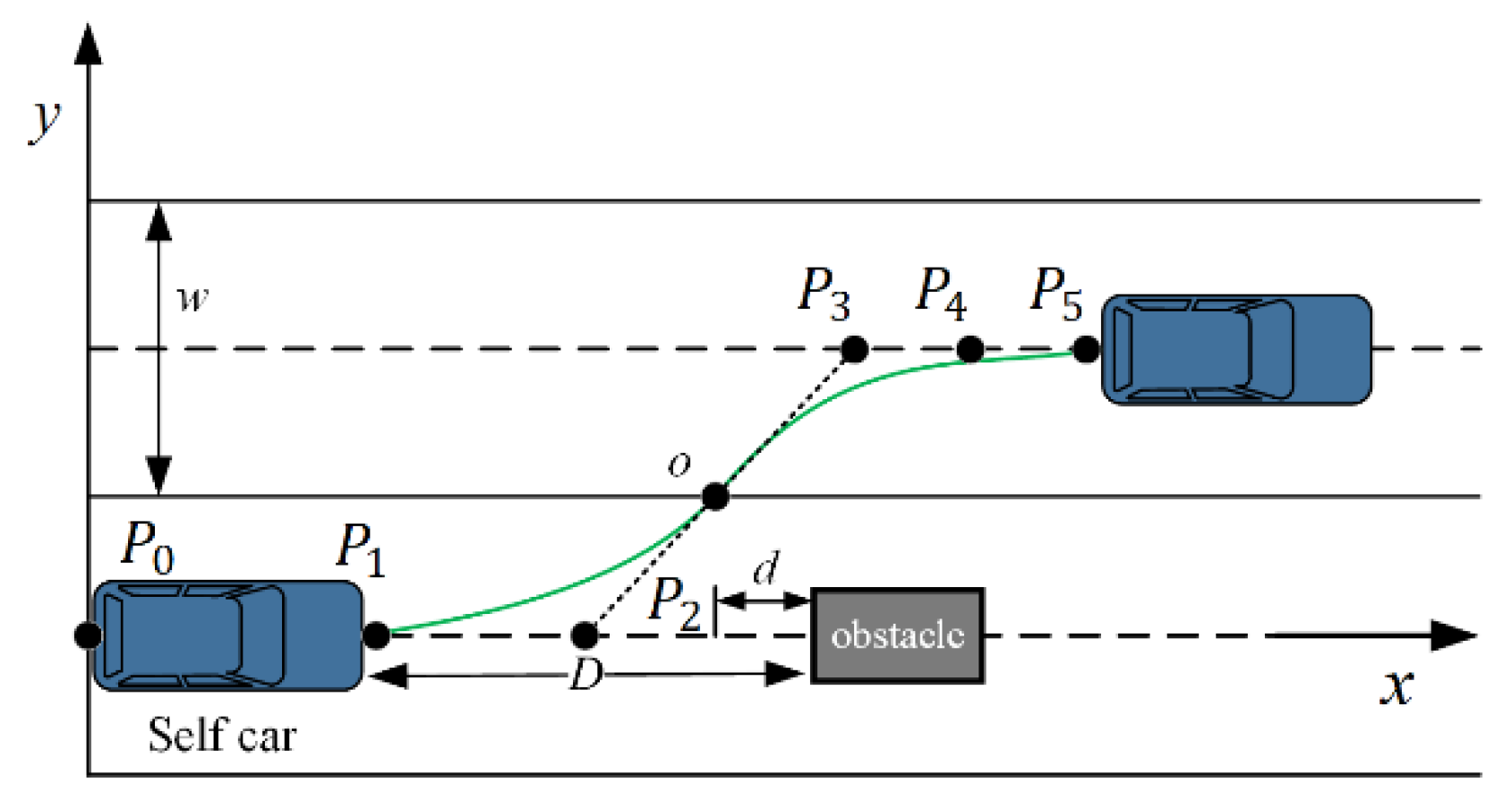
3.1.1. Definition of the Coordinates of Control Points

The position of the control point must be defined in accordance with the nature of the Bezier curve. Therefore, in the structured road scenario when static obstacles exist in front of a vehicle during driving, local path planning is needed to avoid obstacles. The vehicle is assumed to run at a constant speed at the initial time, that the longitudinal speed is $v$ and that the lateral speed and acceleration are zero. The schematic diagram of local path planning is shown in Figure 7.

In Figure 7, blue represents the vehicle, and the grey rectangle represents the stationary obstacle vehicle. $P_0 ~P_5$ are the six control points that determine local path planning. The point $o\left(x_o,y_o\right)$ is the imaginary trajectory symmetry point and is located on the middle route of the two-lane line. The coordinates of each control point can be determined in accordance with the properties of the Bezier curve. The initial heading angle of the vehicle is parallel to the centre line of the lane to meet the requirements that the curvature of the starting and target points is zero. The subsequent lane change of the vehicle is facilitated, and the control points $P_0, P_1, P_2$ and the control points $P_3,P_4, P_5$ are set to be on the same straight line.

The control points $P_0$ and $P_5$, that is, the initial and target points of the lane change of the vehicle, respectively, can then be expressed as:

$$\left\{\begin{array}{l}{P}_0=\left(x_0,y_0\right)=\left(0,0\right)\hfill \\ P_5=\left(x_5,y_5\right)=\left(2x_0,w\right)\hfill \end{array}\right.$$

(16)

where $w$ represents the lane width and is 3.5 m in this work.

In accordance with the symmetry of the vehicle on the road, the first and last three control points of the Bezier curve are set to be symmetrical with respect to the $o$ point. This approach can simplify the algorithm and improve the real-time performance of path planning. By setting $P_1$ as the midpoint of the line segment $P_0$ and $P_2$, $P_4$ as the midpoints of line segments $P_3$ and $P_5$, respectively, the following exist:

$$\left\{\begin{array}{l}{P}_1=\left(x_1,y_1\right)=\left(x_2/2,0\right)\hfill \\ P_4=\left(x_4,y_4\right)=\left(2x_o-x_2/2,w\right)\hfill \end{array}\right.$$

(17)

Given that control points $P_2$ and $P_3$ are symmetric with respect to point $o$, the following exist:

$$\left\{\begin{array}{l}{P}_2=\left(x_2,y_2\right)=\left(x_2,0\right)\hfill \\ P_3=\left(x_3,y_3\right)=\left(2x_o-x_2,w\right)\hfill \end{array}\right.$$

(18)

Considering that various disturbances, such as sideslip and lateral wind, exist during vehicle operation, a safe distance model is established to fully ensure safety during lane changing. Its mathematical expression is:

$$d=v{t}_1+d_0$$

(19)

where $v$ represents the vehicle speed. $t_1$ is the obstacle risk coefficient and is generally between the range of 0~1. $d_0$ is the distance between the car and the obstacle in the emergency stop, that is, the minimum safety distance, and is generally 2~3 m.

In accordance with the above safe distance model, the coordinates of the symmetric point $o$ are set as follows:

$$o\left(x_o,y_o\right)=\left(D-d+a/2,w/2\right)$$

(20)

where $D$ is the initial distance between the vehicle and obstacle to the path planning time and is usually 2~3v, and $a$ is the length of the car body.

The above shows that the longitudinal position coordinate $x_2$ at the control point $P_2$ determines the path shape. The $x_2$ coordinate can then be acquired to obtain the planned path.

3.1.2. Optimal Path Curve Selection

The above indicates that the planned path can be obtained by solving the $x_2$ coordinates. Therefore, this work generates curve clusters in accordance with different $x_2$ values and evaluates each curve by setting a multiobjective evaluation function. The minimum cost function value in the curve cluster is the optimal path curve. The multiobjective function is then:

$$J=\min \left(w_1{J}_1+w_2{J}_2+w_3{J}_3+w_4{J}_4\right)$$

(21)

where $J_1,J_2,J_3,J_4$ represent the sub-optimisation index functions of the optimisation index function. $w_1,w_2,w_3,w_4$ are the weight coefficients of their respective optimisation index functions. The purpose of the above equation is to obtain the optimal planning path with constrained optimisation by weighting parameters and designing their respective optimisation index functions to minimise the optimisation function $J$.

The first sub-optimisation index $J_1$ represents the maximum curvature of the planned path, and as can be known from the vehicle kinematics model, the curvature is positively correlated with the lateral acceleration of a vehicle. A large value of the index $J_1$ is indicative of the greater lateral acceleration of the vehicle. Excessive maximum curvature can easily lead to sideslipping or even the rollover of the vehicle, and a small $J_1$ is indicative of stable vehicle performance. Therefore, this sub-optimisation index can filter out the path with excessive curvature and ensure safety.

The sub-optimisation index $J_2$ is an integral of the first-order differential of the curvature of the planned path to ensure that the curvature of the vehicle’s driving trajectory is derivable. The above shows that a small $J_2$ is indicative of the small curvature mutation of the driving trajectory, a smooth trajectory and improved vehicle stability during driving. $J_2$ is expressed as follows:

$$J_2={\displaystyle \int {\left(\dot{K}\left(s\right)\right)}^{2}ds}$$

(22)

where $K$ denotes the curvature of the local planning path, and $s$ denotes the planning path position corresponding to the curvature $K$.

The sub-optimisation index $J_3$ represents the average curvature of the driving path, which reflects the overall lateral acceleration of the planned path.

$$J_3=\frac{1}{n}{\displaystyle {\int }_0^1{\left(k\right)}^{2}dt}$$

(23)

where $k$ denotes the curvature of all discrete points in the planning path, and $n$ is the number of path points. A small average curvature of the path is associated with a small overall lateral acceleration when the vehicle follows the path and the stable overall yaw performance of the vehicle.

The last sub-optimisation index $J_4$ represents the total length of the planned lane change path, which is used to characterise the lane change time. Given that lane changing by the vehicle is a dangerous condition, the lane change length of the vehicle should be minimised. A short lane change path is also indicative of low time consumption. Therefore, the sub-optimisation index function $J_4$ is used to screen out the path with a short lane change length and low time consumption.

$$J_4={\displaystyle \sum _{i=1}^{n-1}\sqrt{{\left(x_{i+1}-x_i\right)}^2+{\left(y_{i+1}-y_i\right)}^2}}$$

(24)

By adjusting the weight coefficients $w_1,w_2,w_3$ and $w_4$ of the above-defined optimisation objectives, the optimal $x_2$ coordinates corresponding to different vehicle speeds can be obtained, and the optimal driving trajectory curve can be planned.

3.2. Speed Planning Based on Dynamic and Quadratic Programming

Given the uncertainty of the trajectory of a dynamic obstacle, the trajectory may collide with the planned path of a self-driving vehicle at a particular time. If the dynamic obstacle is avoided by the local path planning method, the vehicle is easily induced to produce extreme walking and exhibits incomplete collision avoidance. Furthermore, at high speeds, the vehicle is prone to lateral instability. Therefore, on the basis of the prediction of pedestrian trajectory and the path planning of the main vehicle, this work solves the S–T diagram of the main vehicle and plans a reasonable longitudinal driving speed curve for the main vehicle such that the vehicles can avoid dynamic obstacles safely and comfortably.

3.2.1. Definition of the Pedestrian Collision Boundary

In accordance with the pedestrian social force model, when pedestrians (or obstacles) are present, the collision problem between the car and obstacle must be considered. Given that pedestrians are special agents in traffic, this work takes pedestrian $i$ as the centre of the circle and sets them as the centre. The circle’s radius is 1 m, that is, a circular model with radius $r_i$, and the self-driving car is a geometric circular model with the width of the centre of the head of the car as the diameter of the circle, that is, a circular model with radius $r_v$. During lane changing, the tangent point of the geometric circle between the car and obstacle is the constraint point that prevents collision. The diagram of pedestrian collision boundary is shown in Figure 8.

The calculation formula of the safe lane change distance $S$ considering the pedestrian collision boundary is:

$$S=L_v+r_s$$

(25)

$$L_v=v_{0}t+\frac{1}{2}a{t}^2$$

(26)

$$r_s=r_d\cos \theta$$

(27)

$$r_d=r_v+r_i$$

(28)

where $r_d$ represents the sum of the radii of the vehicle and pedestrian, $\theta$ is the angle from the centre point of the vehicle to the centre point of the pedestrian, $r_s$ is the lateral distance from the centre point of the vehicle to the centre point of the pedestrian, $L_v$ is the distance from the beginning position of the lane change to the limit position of the lane change, $v_0$ is the initial speed when the vehicle begins to change the lane, $a$ is the acceleration during the lane change and $t$ is the time. On the basis of the above definition of a safe lane-changing distance, the safe collision distance boundary is $S\ge L_v+r_s$:

Figure 8. Diagram of the pedestrian collision boundary.

Figure 8. Diagram of the pedestrian collision boundary.

3.2.2. Initial Velocity Planning Based on Dynamic Programming

Although the path generated after path planning can avoid static obstacles, the avoiding of dynamic obstacles needs to be considered in speed planning. The dynamic planning algorithm in the S–T diagram for the initial planning of speed is chosen to obtain the optimal speed profile. In the S–T curve, a slow curve trend is indicative of the low change rate of vehicle displacement, that is, the speed is low. By contrast, if the curve’s trend is steep, the change rate of vehicle displacement is large, that is, the speed is high. Any S–T diagram is based on an already given trajectory curve, and each dynamic obstacle has a projection on this given trajectory in accordance with the vehicle’s prediction module’s trajectory prediction of an obstacle in a dynamic environment. In Figure 9, the red parallelogram is the obstacle area. The rest of the area is the safe area if the car is travelling at a constant speed in accordance with the initial velocity. The blue line in the figure is the unplanned speed curve, which occupies the relationship with the red obstacle area, that is, the car collides with the obstacle. Therefore, in the S–T diagram, only one speed curve that can avoid the obstacle area needs to be planned for the safe area. The green line in the figure is the planned speed curve, which is said to be the S–T curve and can guarantee that the car is travelling safely at a certain time.

Dynamic programming algorithms are generally solved numerically and iteratively. Therefore, the S–T diagram must be the discretisation before solving for the optimal speed by using dynamic programming algorithms. Figure 10 is a schematic diagram of the discretisation of the S–T graph, where $T_{\max }$ is the speed planning time, $S_{\max }$ is the maximum distance that the self-driving car can travel in a speed planning cycle, $\Delta t$ is the time discretisation step and $\Delta s$ is the distance travelled discretisation step.

When solving the optimal speed curve, the dynamic programming starts from the current moment (the current moment defaults to 0 moment) to calculate the value of the initial state to all states at each time point, and the solution order continues backward in time. The value of the initial time $T_0$ to time $T_{i+1}$ is the sum of the optimal cost from the initial time $T_0$ to $T_i$ and the state transition cost from $T_i$ to $T_{i+1}$. After calculating the cost of all states at time $T_{\max }$, the coordinates corresponding to the minimum cost are taken, and the optimal velocity curve can be obtained by backtracking. When solving the optimal speed curve by dynamic programming, the cost function is defined as follows:

$$L\left(s\left(t\right)\right)=w_1{\displaystyle {\int }_{t_0}^{t_{\max }}{\left(s^{\prime }\left(t\right)-v_{ref}\right)}^2}dt+w_2{\displaystyle {\int }_{t_0}^{t_{\max }}{\left(s^{″}\left(t\right)\right)}^2}dt+w_3{\displaystyle {\int }_{t_0}^{t_{\max }}{\left(s^{‴}\left(t\right)\right)}^2}dt+w_{4}Obs\left(s\left(t\right)\right)$$

(29)

The first item in the formula is the speed maintenance cost. In the absence of obstacles in the vehicle’s driving path, the specified speed should be followed, where $v_{ref}$ is the reference speed, the driver or road speed limit and the path curvature. The second and third terms describe the smoothness of the vehicle’s speed profile, which will affect vehicle comfort. The fourth term is the safety cost term, which is defined as follows:

$$Obs\left(s\left(t\right)\right)=\left\{\begin{array}{cc}\frac{d_0-d}{d_0}\hfill & ,d\le d_0\\ \hfill 0\hfill & ,d>d_0\hspace{0.33em}\hfill \end{array}\right.$$

(30)

where $d_0$ represents the safe distance, and $d$ represents the distance between the vehicle and obstacle. When $d$ is greater than $d_0$, the cost is 0. When $d$ is less than $d_0$, the cost is determined by Formula (1).

In the S–T diagram, the selection of feasible state points at each moment needs to meet certain constraints as follows:

$$0\le v\le v_{\max }$$

(31)

$$a_{\min }\le a\le a_{\max }$$

(32)

Equation (31) is the maximum speed constraint, and the vehicle cannot go backwards. Equation (32) comprises the maximum and minimum acceleration constraints. The existence of the constraint condition prevents the dynamic programming algorithm from solving all states at each time when solving the optimal solution such that its speed improves.

3.2.3. Optimised Speed Curve Based on Quadratic Programming

The initial velocity planning by the above dynamic programming method only satisfies obstacle avoidance but not constraints such as the initial state of the vehicle. Therefore, as described in this section, the quadratic programming algorithm is used to optimise the initial planning velocity curve to meet the vehicle’s initial position, velocity and acceleration constraints. Given that the quintic polynomial has the performance of continuous velocity and acceleration and can set constraints at the start and end points, this work defines n quintic polynomials that fit the optimised S–T curve. The expression is as follows:

$$S_i\left(t\right)=a_{0i}+a_{1i}t+a_{2i}{t}^2+a_{3i}{t}^3+a_{4i}{t}^4+a_{5i}{t}^5$$

(33)

where $a_0~a_5$ represent the coefficients of the quintic polynomial, and $t$ is time. The planned velocity $v$ and acceleration curves can be obtained by solving the first and second derivatives of the above formula, respectively. The coefficient of $a$ for the quintic polynomial is the number that minimises the cost function. The cost function is defined as:

$$C_{total}\left(s\right)=w_1{\displaystyle {\int }_{t_0}^{t_{\max }}{\left(s-s_{ref}\right)}^{2}dt+}{w}_2{\displaystyle {\int }_{t_0}^{t_{\max }}{\left(s^{″}\right)}^{2}dt}+w_3{\displaystyle {\int }_{t_0}^{t_{\max }}{\left(s^{‴}\right)}^2}dt$$

(34)

In Equation (34), the first term calculates the distance between the dynamic programming speed navigation contour $s_{ref}$ and the generated path $s$. This term functions to limit the optimal path to a certain area. Regarding the second and third reaction speed smoothness, the cost function balances the navigation line following and smoothness. The relevant constraints need to be set after the cost function is set. The constraints include the initial position, speed and acceleration of the vehicle.

$$\left\{\begin{array}{l}{S}_1\left(0\right)=S_0\hfill \\ v_1\left(0\right)=v_0\hfill \\ a_1\left(0\right)=a_0\hfill \end{array}\right.$$

(35)

where $S_1\left(0\right)$, $v_1\left(0\right)$ and $a_1\left(0\right)$ are the position, velocity and acceleration of the planned S–T curve at the initial moment, respectively. $S_0$, $v_0$ and $a_0$ are the initial position, velocity and acceleration of the vehicle, respectively.

The following equality constraints are defined to ensure continuity between adjacent curves:

$$\left\{\begin{array}{l}{S}_i\left(t_{end}\right)=S_{i+1}\left(0\right)\hfill \\ v_i\left(t_{end}\right)=v_{i+1}\left(0\right)\hfill \\ a_i\left(t_{end}\right)=a_{i+1}\left(0\right)\hfill \end{array}\right.$$

(36)

The following inequality constraints are defined to ensure that the planned polynomial curve is in the feasible region:

$$\left\{\begin{array}{l}{S}_i\left(t\right)\le S_{ub},S_i\left(t\right)\ge S_{lb}\hfill \\ v_i\left(t\right)\le v_{ub},v_i\left(t\right)\ge v_{lb}\hfill \\ a_i\left(t\right)\le a_{ub},a_i\left(t\right)\ge a_{lb}\hfill \end{array}\right.$$

(37)

where $S_{ub}$ and $S_{lb}$ are the upper and lower bounds of position, respectively. $v_{ub}$ and $v_{lb}$ are the upper and lower bounds of velocity, respectively. a_ub and a_lb are the upper and lower bounds of acceleration, respectively.

$$\begin{array}{c}\min J_2=\frac{1}{2}{x}^{T}Gx+c^{T}x\\ s.t A\times x\le b,\\ A_{eq}\times x=b_{eq},\\ lb\le x\le ub.\end{array}$$

(38)

where G represents a positive semidefinite Hesse matrix; x is a quintic polynomial coefficient; A and b are inequality constraint matrices; $A_{eq}$ and b_eq are equality constraint matrices; lb and ub are upper and lower bounds of coefficients. Finally, the QP solving function Quadprog in MATLAB R2020b is used to solve the above quadratic programming equation, and the optimised S–T curve is obtained. The planned velocity and acceleration information can be acquired through derivation.

4. Simulation Experiments Verification and Analysis

A joint simulation model is built by using PreScan8.5.0, CarSim2019.0 and MATLAB R2020b & Simulink, and experimental simulation verification is conducted on the front pedestrian deceleration/uniform driving scenario to verify the feasibility, rationality and effectiveness of the proposed method for intelligent vehicle motion planning based on trajectory prediction. PreScan8.5.0 builds a vehicle simulation scene and provides the sensor data of the main vehicle. These data include the driving parameters, such as the position, speed and acceleration, of the interactive vehicle in the scenario. CarSim2019.0 provides the vehicle dynamics model. MATLAB R2020b & Simulink builds the vehicle path planning, speed planning and vehicle control algorithm model.

Figure 11 shows that in the forward pedestrian deceleration or uniform speed scenario, the intelligent vehicle motion planning based on proposed trajectory prediction is combined with simulation verification. The middle line in the figure is the optimal trajectory planned by the intelligent vehicle because Pedestrian 1 keeps self-driving at a constant speed when a car is present at their rear. By contrast, Pedestrians 2 and 3 interact. In addition, Pedestrians 2 and 3 decelerate at the rear, whereas Pedestrian 4 crosses the road. Given the long distance from the intelligent vehicle, Pedestrian 4 continues self-driving at a constant speed. Therefore, the vehicle chooses to avoid Pedestrians 1, 2 and 3 in advance to ensure driving safety and comfort and the predicted trajectory. When Pedestrian 4 approaches the intelligent vehicle in accordance with the predicted trajectory, the vehicle moves to the upper lane such that it switches to the main lane to avoid Pedestrian 4.

Considering that the vehicle is driving behind the pedestrian, the pedestrian is in a uniform or decelerated driving state. In accordance with the above trajectory prediction, the pedestrian can know the future trajectory direction, that is, the pedestrian’s speed position is known such that the vehicle can consider the appropriate position for changing lanes to avoid the pedestrian, thus presenting a safe lane change path and speed. In the scenario in which the pedestrian decelerates or maintains uniform speed at the front of the vehicle, human–human and human–vehicle interactions occur such that the simulated virtual scenario is close to the situation encountered by the vehicle on the road in the real scenario. The initial speed and initial acceleration of the vehicle are set to 0, and the vehicle position is (3, 11). The average speed of pedestrians is set to 1.1 m/s, and the deceleration is set to 0.5 m/s². In this work, pedestrians decelerate or maintain their speed in accordance with the driving position of the vehicle. Given the need to ensure pedestrian safety, when pedestrians are present in front of the vehicle, the vehicle slows down first and then decides to accelerate to change lanes and avoid pedestrians in accordance with the predicted future position of pedestrians. The pedestrian trajectory is predicted in accordance with the improved pedestrian social force model described in the first section of this paper. The predicted pedestrian trajectory is shown in Figure 12.

In the above scenario, the motion of the intelligent vehicle is planned in accordance with the pedestrian’s predicted trajectory. In intelligent vehicle motion planning, the intelligent vehicle firstly completes the usual start process and drives on the lane. The path and speed of the intelligent vehicle are determined in accordance with the pedestrian position speed detected by the sensor and then the optimal motion trajectory curve is obtained, as shown in Figure 13.

The speed curve, longitudinal acceleration curve, lateral acceleration curve and heading angle curve are shown in Figure 14, Figure 15, Figure 16 and Figure 17. The difference between the algorithm proposed in this paper and traditional algorithm that does not consider the pedestrian trajectory prediction is described below.

When Pedestrian 1 walks at a constant speed, the intelligent vehicle chooses to avoid collision with great longitudinal acceleration in consideration of pedestrian trajectory. This situation occurs because Pedestrian 1 is moving at a constant speed. The intelligent vehicle can acquire further safe distance and chooses to accelerate in the left lane and then reduces its acceleration to change lanes to avoid collision. During the turning process, the lateral acceleration curve was comparatively smooth because the vehicle adjusts the angle at any time in accordance with the pedestrian trajectory. As to the traditional algorithm, the vehicle continues to accelerate and successfully turns to avoid collision before encountering pedestrians, but it does not slow down during the turning process. The relative safety distance is small, putting pedestrians in dangerous areas and having poor vehicle stability. It shows that the safe distance between pedestrians and vehicles can be guaranteed when considering the future trajectory of Pedestrian 1, and the comfort and path smoothness of intelligent vehicle lane change can be guaranteed.

Pedestrians 2 and 3 are decelerating, and human–human and human–vehicle interactions exist. When considering trajectory prediction, the speed curve shows that the intelligent vehicle starts speed planning from 8 s to 11 s. At the end of speed planning, Pedestrian 2 and Pedestrian 3 are predicted to decelerate, and the longitudinal acceleration curve begins to decrease from longitudinal acceleration at 8 s such that the speed change reduces. Therefore, during steering, the vehicle can ensure that it does not collide with the decelerating pedestrians, thus ensuring pedestrian safety. Considering that the smart car has just changed lanes to avoid Pedestrian 1 in the right lane, the change rate of lateral acceleration must be high to make the vehicle return to the left lane to avoid collision with Pedestrians 2 and 3. However, as to the traditional algorithm, the vehicle continues to accelerate after avoiding Pedestrian 1. Because the future trajectory of the pedestrian in front is unknown and the speed is fast, it does not avoid the pedestrian in time and collides with the pedestrian.

When Pedestrian 4 walks at a constant speed and the left lane is the destination, the pedestrian trajectory prediction diagram shows that the pedestrian is in the left-lane position at this time. Therefore, the intelligent vehicle needs to make a lane change decision to avoid Pedestrian 4 when it is approaching Pedestrian 4. The speed curve below shows that the curve considering trajectory prediction makes a lane change avoidance decision by reducing speed. The longitudinal acceleration curve of the intelligent vehicle also gradually decreases. The intelligent vehicle without considering the trajectory prediction collides with Pedestrian 2 and Pedestrian 3. The intelligent vehicle fails to change lanes in time, and its position is still in the right lane. Pedestrian 4 has no effect on the intelligent vehicle without considering the trajectory prediction, so the intelligent vehicle planning ends at the expected speed.

5. Conclusions

The proposed method for pedestrian trajectory prediction with an improved social force model can predict the future trajectory of pedestrians when their position and velocity are continuously recursive by time step driven by combined social forces until a trajectory is generated after 2 s when initial conditions are given. Subsequently, intelligent vehicle motion planning is proposed on the basis of pedestrian trajectories. Path planning is based on fifth-order Bezier curves. Speed planning is performed through dynamic and quadratic planning. Moreover, the pedestrian collision boundary is proposed in speed planning, which defines pedestrians and vehicles as circular models such that the absolute safety of pedestrians can be ensured during planning. Finally, the front pedestrian deceleration or uniform speed driving scenario is simulated, wherein the highest vehicle speed is 6.39 m/s under the premise of ensuring pedestrian safety and the average speed of the intelligent vehicle after a normal start is 4.6 m/s, thus meeting the driving state required by intelligent vehicles in reality. The results show that using the fifth-order Bezier curve can effectively improve the smoothness of the path and can ensure the continuity of curvature without curvature mutation and difficulty in balancing the shape of the curve. This study could provide a theoretical basis and supporting method for human–vehicle interactions and the safety decision-making of autonomous vehicles in complex environments. However, this work does not analyse pedestrian intention prediction and the motion planning problem in multifactor traffic scenarios. In the future, further research will be conducted on decision-making planning on the basis of integrating vehicle safety, energy savings and high efficiency under the coupled mechanism of pedestrian behavioural characteristics and the vehicle–road–pedestrian cycle.

References

1. Yang, S.; Cao, Y.; Peng, Z.; Wen, G.; Guo, K. Distributed formation control of nonholonomic autonomous vehicle via RBF neural network. Mech. Syst. Signal Process. 2016, 87, 81–95. [Google Scholar] [CrossRef]
2. Zhang, H.; Wang, R.; Wang, J. H-infinity Observer Design for LPV Systems with Uncertain Measurements on Scheduling Variables: Application to an Electric Ground Vehicle. IEEE/ASME Trans. Mechatron. 2016, 21, 1659–1670. [Google Scholar] [CrossRef]
3. Yurtsever, E.; Lambert, J.; Carballo, A. A Survey of Autonomous Driving: Common Practices and Emerging Technologies. IEEE Access 2020, 8, 58443–58469. [Google Scholar] [CrossRef]
4. Abudayyeh, D.; Almomani, M.; Almomani, O.; Alsoud, H.; Alsalman, F. Perceptions of Autonomous Vehicles: A Case Study of Jordan. World Electr. Veh. J. 2023, 14, 133. [Google Scholar] [CrossRef]
5. Rudenko, A.; Palmieri, L.; Herman, M.; Kitani, K.M.; Gavrila, D.M. Human Motion Trajectory Prediction: A Survey. Int. J. Robot. Res. 2019, 39, 895–935. [Google Scholar] [CrossRef]
6. Claussmann, L.; Revilloud, M.; Gruyer, D.; Glaser, S. A review of motion planning for highway autonomous driving. IEEE Trans. Intell. Transp. Syst. 2019, 21, 1826–1848. [Google Scholar] [CrossRef]
7. Song, H.; Ding, W.; Chen, Y.; Shen, Q. PiP: Planning-Informed Trajectory Prediction for Autonomous Driving. European Conference on Computer Vision; Springer: Berlin/Heidelberg, Germany, 2020; pp. 598–614. [Google Scholar]
8. Lee, N.; Choi, W.; Vernaza, P.; Choy, C.B.; Torr, P.H.S.; Chandraker, M. Desire: Distant Future Prediction in Dynamic Scenes with Interacting Agents. In Proceedings of the 2017 IEEE Conference on Computer Vision and Pattern Recognition, Honolulu, HI, USA, 21–26 July 2017; pp. 336–345. [Google Scholar]
9. Leon, F.; Gavrilescu, M. A review of tracking and trajectory prediction methods for autonomous driving. Mathematics 2021, 9, 660. [Google Scholar] [CrossRef]
10. Helbing, D.; Molnar, P. Social force model for pedestrian dynamics. Phys. Rev. E 1995, 51, 4282–4286. [Google Scholar] [CrossRef]
11. Helbing, D.; Farkas, I.; Vicsek, T. Simulating dynamical features of escape panic. Nature 2000, 407, 487–490. [Google Scholar] [CrossRef]
12. Luber, M.; Stork, J.A.; Tipaldi, G.D.; Gian, D.; Arras, K.O. People tracking with human motion predictions from social forces. In Proceedings of the 2010 IEEE International Conference on Robotics and Automation, Anchorage, AK, USA, 3–7 May 2010; pp. 464–469. [Google Scholar]
13. Alahi, A.; Ramanathan, V.; Li, F.F. Socially-aware large-scale crowd forecasting. In Proceedings of the 2014 IEEE Conference on Computer Vision and Pattern Recognition, Columbus, OH, USA, 23–28 June 2014; pp. 2211–2218. [Google Scholar]
14. Yi, S.; Li, H.S.; Wang, X.G. Understanding pedestrian behaviors from stationary crowd groups. In Proceedings of the 2015 IEEE Conference on Computer Vision and Pattern Recognition, Boston, MA, USA, 7–12 June 2015; pp. 3488–3496. [Google Scholar]
15. Qu, Z.W.; Cao, N.B.; Chen, Y.H.; Zhao, L.Y.; Luo, R.Q. Modeling electric bike–car mixed flow via social force model. Adv. Mech. Eng. 2017, 9, 1–14. [Google Scholar] [CrossRef]
16. Zhang, X.; Chen, H.; Yang, W.; Jin, W.; Zhu, W. Pedestrian path prediction for autonomous driving at un-signalized crosswalk using W/CDM and MSFM. IEEE Trans. Intell. Transp. Syst. 2021, 22, 3025–3037. [Google Scholar] [CrossRef]
17. Rasouli, A.; Tsotsos, J.K. Autonomous Vehicles That Interact with Pedestrians: A Survey of Theory and Practice. IEEE Trans. Intell. Transp. Syst. 2020, 21, 900–918. [Google Scholar] [CrossRef]
18. Song, X.; Gao, H.; Ding, T.; Gu, Y.; Liu, J.; Tian, K. A Review of the Motion Planning and Control Methods for Automated Vehicles. Sensors 2023, 23, 6140. [Google Scholar] [CrossRef] [PubMed]
19. You, C.; Lu, J.; Filev, D.; Tsiotras, P. Autonomous planning and control for intelligent vehicles in traffic. IEEE Trans. Intell. Transp. Syst. 2019, 21, 2339–2349. [Google Scholar] [CrossRef]
20. Chen, L.; Qin, D.; Xu, X.; Cai, Y.; Ju, X. A path and velocity planning method for lane changing collision avoidance of intelligent vehicle based on cubic 3-D Bezier curve. Adv. Eng. Softw. 2019, 132, 65–73. [Google Scholar] [CrossRef]
21. Brezak, M.; Petrovic, I. Real-time approximation of clothoids with bounded error for path planning applications. IEEE Trans. Robot. 2014, 30, 507–515. [Google Scholar] [CrossRef]
22. Wang, Z.; Peng, R.; Gong, Z. B-spline curve generation principle and implementation. J. Shihezi Univ. 2009, 27, 118–121. [Google Scholar]
23. Zhang, B.; Li, Z.; Ni, Y.; Li, Y. Research on Path Planning and Tracking Control of Automatic Parking System. World Electr. Veh. J. 2022, 13, 14. [Google Scholar] [CrossRef]
24. Wang, P.; Yang, J.; Zhang, Y.; Wang, Q.; Sun, B.; Guo, D. Obstacle-Avoidance Path-Planning Algorithm for Autonomous Vehicles Based on B-Spline Algorithm. World Electr. Veh. J. 2022, 13, 233. [Google Scholar] [CrossRef]
25. Wenda, X.; Junqing, W.; Dolan, J.M.; Huijing, Z.; Hongbin, Z. A real-time motion planner with trajectory optimization for autonomous vehicles. In Proceedings of the 2012 IEEE International Conference on Robotics and Automation, Saint Paul, MN, USA, 14–18 May 2012; pp. 2061–2067. [Google Scholar]
26. Gonzalez, D.; Perez, J.; Lattarulo, R.; Milanes, V.; Nashashibi, F. Continuous curvature planning with obstacle avoidance capabilities in urban scenarios. In Proceedings of the 17th International IEEE Conference on Intelligent Transportation Systems (ITSC), Qingdao, China, 8–11 October 2014; pp. 1430–1435. [Google Scholar]
27. Latip, N.B.A.; Omar, R. Feasible path generation using bezier curves for car-like vehicle. IOP Conf. Ser. Mater. Sci. Eng. 2017, 226, 012133. [Google Scholar] [CrossRef]
28. Xu, L.; Cao, M.Y.; Song, B.Y. A new approach to smooth path planning of mobile robot based on quartic Bezier transition curve and improved PSO algorithm. Neurocomputing 2022, 473, 98–106. [Google Scholar] [CrossRef]
29. Bae, I.; Moon, J.; Park, H.; Kim, J.H.; Kim, S. Path generation and tracking based on a Bézier curve for a steering rate controller of autonomous vehicles. In Proceedings of the 16th International IEEE Conference on Intelligent Transportation Systems (ITSC 2013), The Hague, The Netherlands, 6–9 October 2013; pp. 436–441. [Google Scholar]
30. Li, M.; Shi, F.; Chen, D. Analyze bicycle-car mixed flow by social force model for collision risk evaluation. In Proceedings of the 3rd International Conference on Road Safety and Simulation, Indianapolis, IN, USA, 14–16 September 2011; pp. 1–22. [Google Scholar]
Figure 1. Schematic diagram of self-driving force.
Wevj 14 00320 g001
Figure 2. Schematic diagram of the force between pedestrians.
Wevj 14 00320 g002
Figure 3. Schematic diagram of pedestrian anisotropy.
Wevj 14 00320 g003
Figure 4. Schematic diagram of pedestrian–vehicle interaction force.
Wevj 14 00320 g004
Figure 5. Road boundary constraints.
Wevj 14 00320 g005
Figure 6. The fifth-order Bezier curve trajectory diagram.
Wevj 14 00320 g006
Figure 7. The schematic diagram of local path planning.
Wevj 14 00320 g007
Figure 9. S–T diagram and speed planning diagram.
Wevj 14 00320 g009
Figure 10. Dynamic programming discretisation schematic diagram.
Wevj 14 00320 g010
Figure 11. Diagram of intelligent vehicle motion planning in the scenario of forward pedestrian deceleration or uniform speed.
Wevj 14 00320 g011
Figure 12. Pedestrian trajectory prediction diagram.
Wevj 14 00320 g012
Figure 13. Optimal motion trajectory curve.
Wevj 14 00320 g013
Figure 14. Speed curve.
Wevj 14 00320 g014
Figure 15. Longitudinal acceleration curve.
Wevj 14 00320 g015
Figure 16. Lateral acceleration curve.
Wevj 14 00320 g016
Figure 17. Heading angle curve.
Wevj 14 00320 g017
Disclaimer/Publisher’s Note: The statements, opinions and data contained in all publications are solely those of the individual author(s) and contributor(s) and not of MDPI and/or the editor(s). MDPI and/or the editor(s) disclaim responsibility for any injury to people or property resulting from any ideas, methods, instructions or products referred to in the content.