1. Introduction
Autonomous vehicles or self-driving cars have been proposed recently over the road network. They are also known as driverless vehicles that can operate and execute vital activities without the assistance of humans [
1]. Thus, these vehicles should be able to investigate their surrounding environment accurately. Several systems have been developed to improve the performance of autonomous vehicles in several road scenarios and situations. Some systems have been designed to drive under bad weather conditions (i.e., fog, rain, snow) [
2,
3,
4]. Other systems have been developed to clearly and accurately control the vehicles at curving roads, junctions, traffic lights, blind turns, and on-street parking [
5,
6,
7,
8,
9,
10].
On the other hand, many researchers have worked on object detection and classification problems over the road network (i.e., regular vehicles, emergency vehicles, cyclists, trucks, pedestrians, etc.) [
11,
12,
13,
14,
15]. These studies effectively aim to reduce the increasing number of traffic accidents over road networks. They also reduce the driver’s stress and tension during their trips [
16]. More importantly, they aim to help ultimately replace the drivers in autonomous vehicle scenarios. The surrounding environment of autonomous vehicles is essential for safe road network trips. Investigating the existing objects should be accurate and quick to avoid crashes and accidents. The system of autonomous vehicles is based mainly on perception and decision-making processes. For example, the route of autonomous vehicles toward the targeted destinations should be set based on some predefined parameters. This includes the physical location of the destination, the map of the surrounding road network, and the navigation trip on the road network [
17,
18].
Quick responses and actions are required from autonomous vehicles upon detecting any object over the road network. These responses depend mainly on the main characteristics of the detected object. Determining the main features of the existing objects: their nature, location, and size is one of the most critical problems that require further development in the system of autonomous vehicles. For instance, vehicles have to decrease their speed to increase the in-between safe distances if a nearby vehicle is detected traveling in front of them. They must change their traveling lane and open the way for emergency vehicles if they are seen behind them. Moreover, warning signs on the road should be analyzed and understood to react accordingly by following the recommended speed or noticing the existing exit point. Detecting a located traffic light at a signalized road intersection determines whether that vehicle can pass through that intersection or it should wait for the green signal.
Machine learning (ML) techniques, such as deep convolution neural networks, have been used in computer vision to detect objects over the road network. The object detection problem over the road network has been handled by analyzing the road’s closed-circuit television (CCTV) footage. With the help of a CCTV camera, images are taken every second. Thus, every vehicle on the road is detected in every image. These studies have classified objects after detecting them [
19]. Processing images acquired robust light detection and extended-range equipment. Moreover, some research studies have focused on the correlated problem of vehicle sensor location problem [
20,
21,
22,
23,
24,
25]. Besides, LiDAR and radar technologies can generate a map of its environment to detect, locate, and track moving targets [
26]. Vehicles, pedestrians, bicycles, motorcycles, and other obstacles on or beside roads are all objects of interest in automotive driving applications [
26]. Thus, radars provide direct perception-related inputs by extracting depth-related characteristics with highly predictable processing approaches. Then, RGB cameras are used to create images that replicate human vision, capturing light in red, green, and blue wavelengths. Processing these images can help to identify existing objects, differentiate them from the background, and analyze a scene. On the other hand, the Global Positioning System (GPS) helps in the navigation system of these vehicles by determining the longitude, latitude, speed, and direction of each vehicle.
In this work, we aim to use data classification techniques as an intelligent object classification approach. This is to classify the detected objects according to their main characteristics. We have investigated the performance of these techniques based on several datasets. Then, collecting several considered objects into three main groups based on the mobility nature of these objects (i.e., vehicles, people, and signs) is applied. The the grouped datasets obtained better Accuracy, Precision, F1-Score, G-Mean, and Recall results. We compare the performance of six main machine learning algorithms to recommend the most suitable one for object detection on road networks. The performance of the proposed approach has been improved by modifying the datasets and grouping similar objects in a single group.
The rest of this paper is organized as follows:
Section 2 investigates some recent relevant studies about object detection and classification in autonomous driving scenarios.
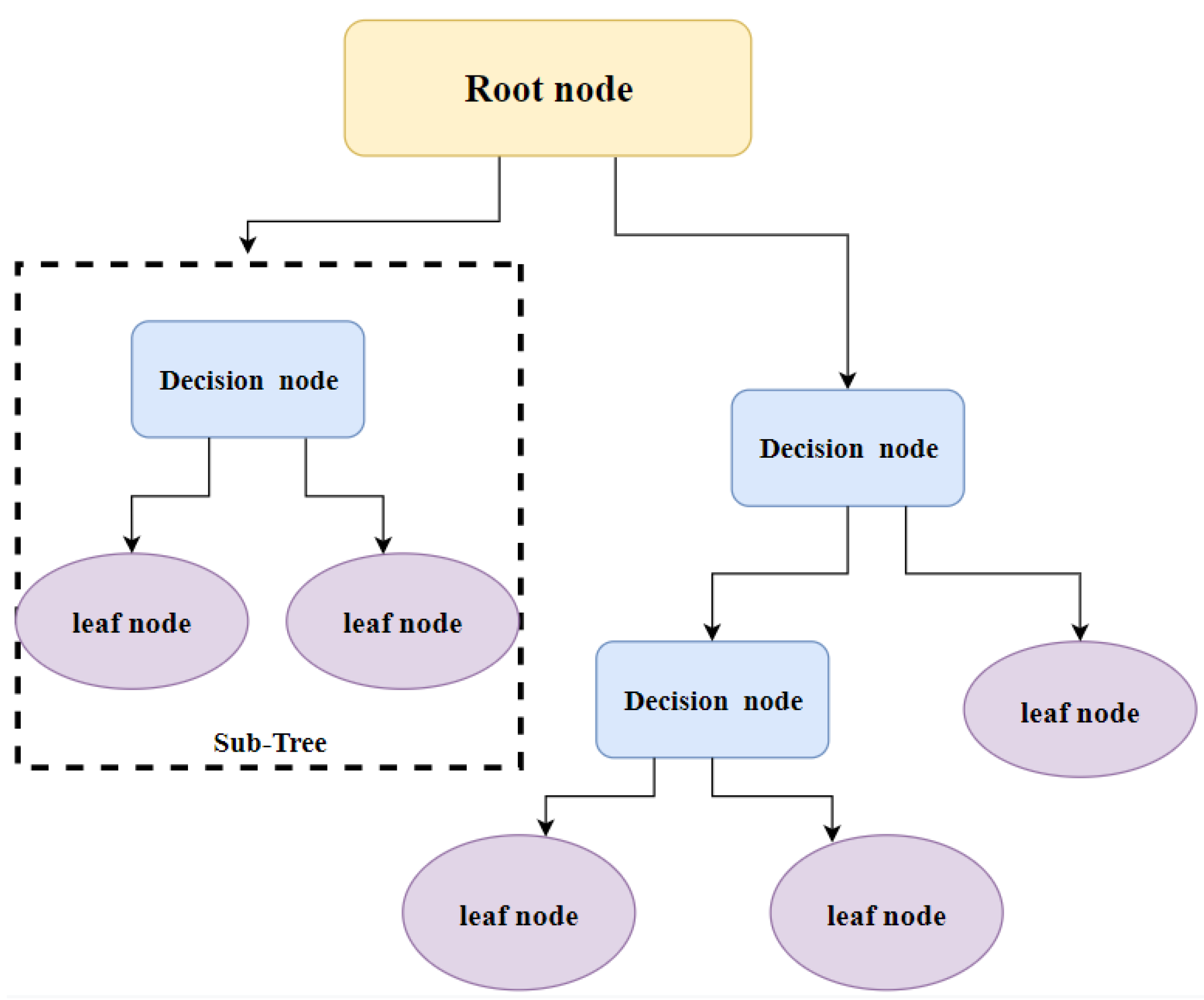
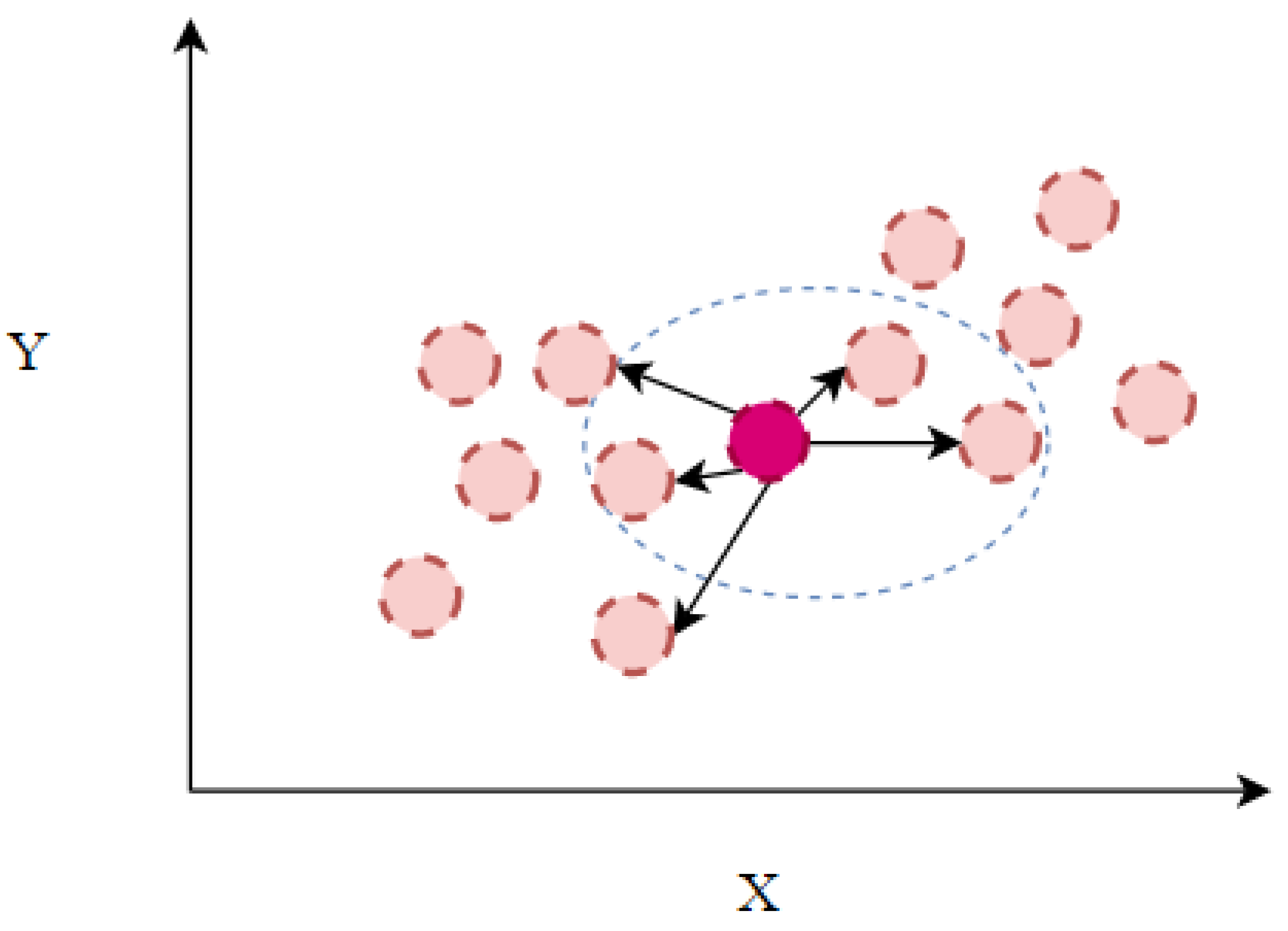
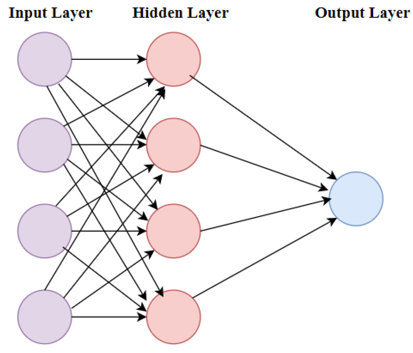
Section 3 provides a brief discussion of the classification algorithms utilized in this work.
Section 4 presents the pre-processing techniques we applied to prepare the dataset. In
Section 5, the experiments and results are presented, discussed, and compared to previous studies. Finally,
Section 6 concludes the entire paper.
2. Literature Review
Object classification is a method of determining which class instances an object belongs to. Autonomous vehicles must classify objects over the road network to take different actions with different existing objects. Moreover, the location of each detected object should be precisely determined. To obtain a complete 3D perspective of the area, object detection is becoming a subdomain of computer vision (CV) [
27]. Among the goals of self-driving cars include saving lives and increasing safety by minimizing accidents, as well as making private transportation possible, efficient, and reliable [
28,
29]. Specific object recognition is a sub-problem of the general object recognition problem. This requires assigning distinguishing attributes to each object with proper names [
30]. Three-dimensional object detection is a crucial task for the autonomous driving of an optical navigation module. Various sensors, such as millimeter-wave radar, camera, or laser radar (LiDAR), provide road scene information to the optical navigation module. Then, classification techniques process the gathered information to give a derivable area for autonomous vehicles [
31]. Udacity presented the dataset generated from the GTI (Grupo de Tratamiento de Imágenes, Madrid, Spain) vehicle image collection and the KITTI (Karlsruhe Institute of Technology, Karlsruhe, Germany and Toyota Technological Institute, Nagoya, Japan) vision benchmark suite. It employs a histogram of oriented gradients (HOG) feature extraction algorithm to recognize multiple vehicles in images and classify them using various classification techniques. The experimental result shows that the efficiency is higher while using the LR when compared to the decision tree (DT) algorithm and the support vector machine (SVM) [
32].
Ortiz Castelló et al. have evaluated version 3 of the “You Only Look Once” (YOLOv3) and YOLOv4 networks by training them on a large, recent, on-road image large-scale Berkeley Deep Drive (BDD100K) dataset, with a significant improvement in detection quality. Additionally, some models were retrained by replacing the original Leaky Rectified Linear Unit (Leaky ReLU) convolution activation functions from the original YOLO implementation with two advanced activation functions. The self-regularized non-monotonic function (MISH) and its self-gated counterpart (SWISH) resulted in significant improvements in detection performance over the original activation function. YOLO is a real-time object detection algorithm that identifies specific objects in videos or images. YOLO uses features learned by a deep convolutional neural network to classify each object. The BDD100K dataset was used to train the algorithms. It is a large, comprehensive dataset that includes a variety of objects in various weather conditions, locations, and times of day, as well as a wide range of light conditions and occlusion. Average Precision (AP) is the primary measure used in this comparison study. The MISH model gets the best performance, followed by the SWISH function. However, both lead to better results than the original Leaky ReLU implementation [
27].
Moreover, deep convolutional networks are used to classify objects accurately by Mobahi and Sadati [
29]. This study used the BDD100K dataset to train and test the algorithm using Python and the open-source PyTorch platform using the CUDA tool, which allows image processing. The experiments were performed using a single-shot multi-box detector (SSD), faster R-CNN (Region-Based Convolutional Neural Network), and PyTorch algorithms. They classified three scales of objects: small, medium, and large [
29]. Karlsruhe Institute of Technology, Toyota Technological Institute (KITTI), and Multifog KITTI datasets have been used in other experimental studies. Mainly, the AP measure has been determined to compute the performance of the 3D object detection task. The findings were greatly enhanced by employing a Spare LiDAR Stereo Fusion Network (SLS-Fusion) [
2]. Then, the proposed 3D object detection algorithm divides objects into three difficulty levels: easy, moderate, and hard. Based on the 2D bounding box sizes, occlusion, and truncation extents appearing on the image. The hard level focuses on classifying objects in foggy weather for self-driving vehicles [
2].
Furthermore, Mirza et al. used YOLOv3, PointPillars, and AVODS (Aggregate View Object Detection) methods to detect and classify objects over the road network. These methods perform much better on the KITTI dataset than the NuScenes, Way Forward in Mobile (Waymo, Mountain View, CA, USA), and A*3D datasets. On night scenes, the mean Average Precision (mAP) achieved by PointPillars is the best. However, it fails in adverse weather situations such as rain [
4]. Then, to increase the performance of classifying objects in foggy weather circumstances, Mai et al. trained the Spare LiDAR Stereo Fusion Network (SLS-Fusion) using the KITTI dataset (i.e., the Multifog KITTI dataset). In addition, Al-Rifai has used the YOLOv3 algorithm with Darknet-53 CNN for object classification on the road network; they detect and classify cars, trucks, pedestrians, and cyclists [
13]. On the other hand, Krizhevsky et al. [
33] proposed a deep convolutional neural network that has been used to extract the image representations automatically. The perception system of an autonomous vehicle converts sensory data into semantic information, such as lane marking, drivable areas, and traffic sign information. Moreover, this system has been developed to identify and recognize objects on the road (e.g., vehicles, pedestrians, cyclists) [
34]. Cameras can recognize pedestrians using a convolutional neural network (CNN) and determine vehicle positions by merging the picture position with the LiDAR point cloud [
35]. Deep learning can be used to process the sounds of emergency vehicles from a long distance and determine the direction from which they are approaching. Autonomous vehicles must notice the responding emergency vehicles [
36].
On real and synthetic data, 3D object detection and classification are implemented by Agafonov and Yumaganov [
37]. Vehicles are used as detected objects, the KITTI dataset is used, and the open-source simulator Consul Auditing and Reporting Language (CARLA) is used as a source of synthetic data. This simulator is provided for testing diverse traffic situations to train autonomous vehicle control systems. The AP of classification objects is measured for these scenarios as an evaluation measure [
37].
Table 1 summarizes the recent studies in object classification mechanisms over the road network, illustrating their main findings and limitations. After looking over the most recent and pertinent studies, we may summarize the deficiencies and weaknesses as follows:
Some investigations produced results that showed a considerable increase in the amount of time needed for processing.
Some studies fail in adverse weather situations such as rain.
They did not perform well in the classification of large-scale objects.
When it comes to categorizing large-scale items, several of the earlier studies did not perform particularly well.
Some studies have a high misclassification rate for small objects compared to larger ones.
There is still room for improving the accuracy measures achieved by the current studies, which results in a higher overall quality of the findings.
This research seeks to design an intelligent object classification approach for autonomous vehicles, as well as provide an efficient model to address these weaknesses.
4. The Proposed Object Detection Approach for Autonomous Vehicles
In this section, we start by discussing the methodology of the proposed approach.
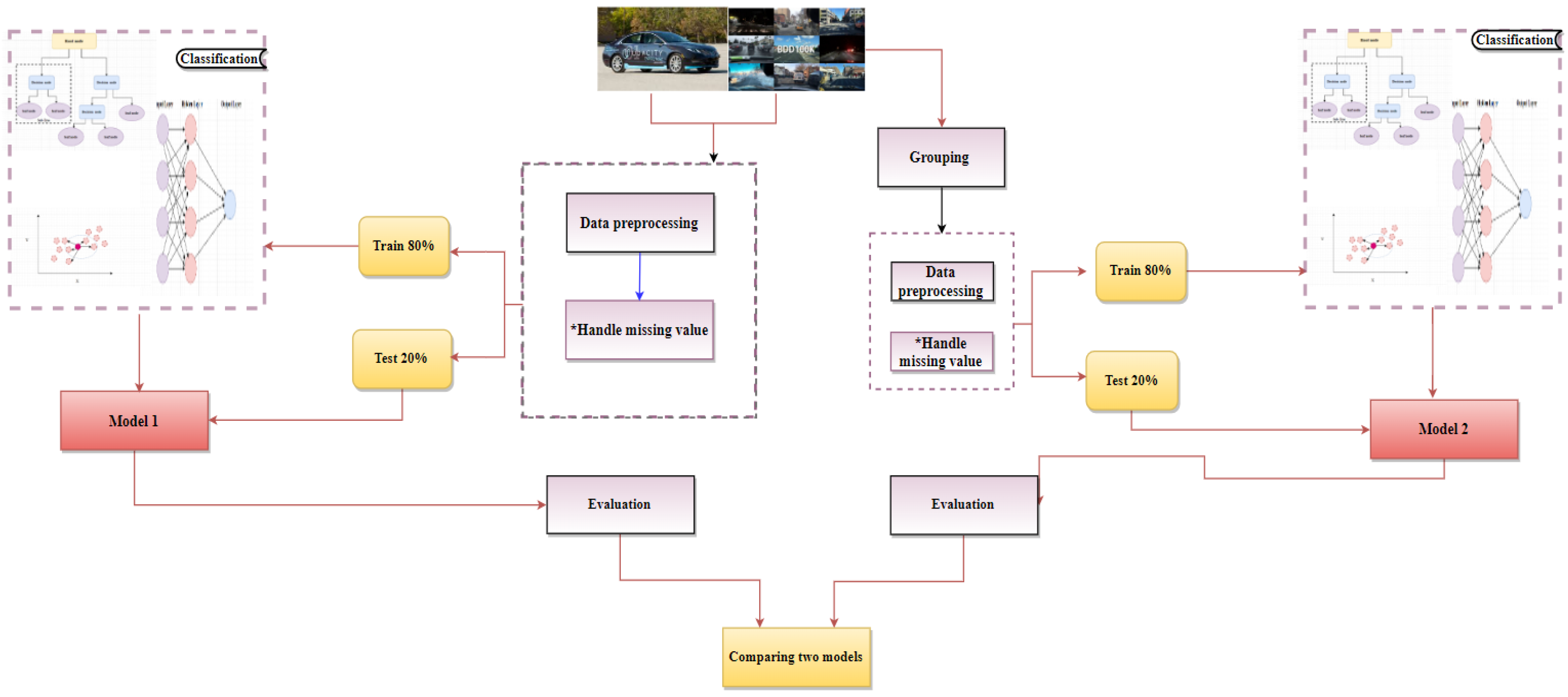
Figure 4 illustrates the steps of the proposed approach methodology. The Udacity and BDD100K datasets are collected from Roboflow and Kaggle repositories. Data preprocessing techniques are applied to handle the missing values in the datasets. In addition, the datasets are split into 80% training data and 20% testing data. The most popular ML mechanisms, such as the DT, NB, KNN, SGD, MLP, and LR algorithms, are used to classify the objects for the Udacity and BDD100K datasets. Finally, the five main evaluation measures for evaluating a classification model are Accuracy, Precision, F1-Score, G-Mean, and Recall. In the second stage, we divided the BDD100K dataset into groups, and the steps mentioned above were re-applied to these groups to obtain a new model compared to the model produced from the first stage.
We provide the procedure followed in preparing and cleaning the used datasets. The imbalanced data issue is discussed as its effects on the obtained results. Making the data more complete and getting more accurate results can be achieved by preprocessing the data. The data preparation process comprises executing Python code to find missing and duplicated values. Every class has a numeric value in the Udacity and BDD100K datasets. The data preprocessing techniques are applied to handle the missing values in the Udacity and BDD100K datasets. Then, the datasets are split into 80% as training and 20% as testing data. The classification algorithms are applied to classify the dataset. Finally, the measures for the algorithms are calculated. The main categories in the Udacity dataset include pedestrian, car, truck, traffic light, and biker. In contrast, the BDD100K dataset includes pedestrian, rider, car, truck, bus, motorcycle, bicycle, traffic light, and traffic sign categories. We can see that the BDD100K is much more sophisticated compared to the Udacity dataset.
4.1. Data Collection
The Udacity dataset was collected using Udacity’s self-driving car simulator [
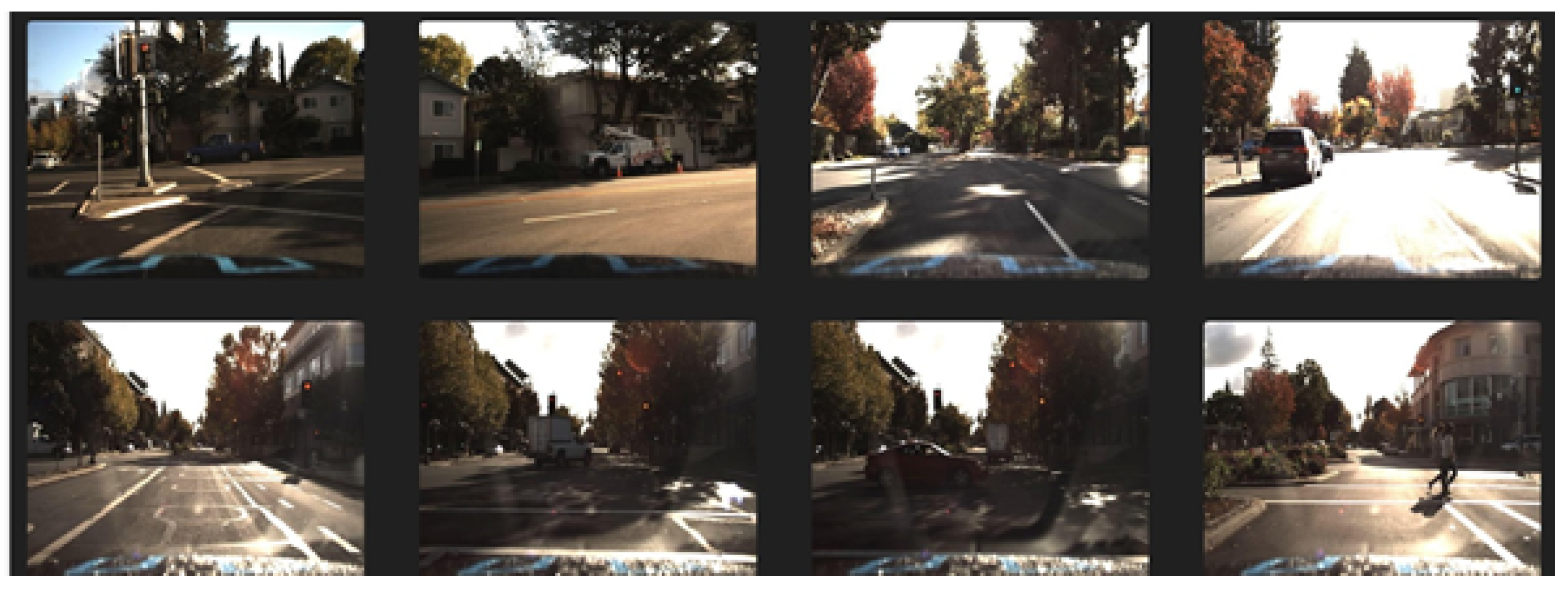
47]. With this simulator’s training mode, drivers can record themselves driving the car on certain tracks. This method is called “behavioral cloning” because it copies the user’s actual actions as they navigate the vehicle. The information is shown as images taken from three angles, mainly from the center, left, and right. The dataset contains 97,942 labels across 11 classes and 15,000 images, including thousands of pedestrians, bikers, cars, and traffic lights. This dataset was exported via Roboflow [
48].
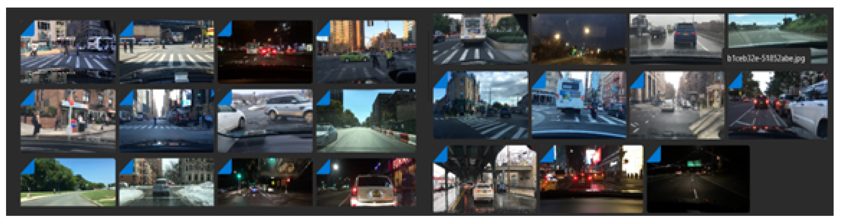
On the other hand, the BDD100K dataset is one of the most commonly used datasets for object detection and classification in autonomous driving. The diversity of the data is essential to test the robustness of perception algorithms. This dataset includes a wide range of scene types, including city streets, residential areas, and highways. In addition, the videos were taken in a wide range of climatic conditions and at various times throughout the day. In this dataset, there are up to 90 objects per image [
29]. The BDD100K dataset contains 13 classes (i.e., traffic sign, traffic light, pedestrian, rider, car, bus, truck, train, motorcycle, bicycle, vehicle, another person, and trailer). General snapshots consisting of several selected images taken from the Udacity and BDD100K datasets are shown in
Figure 5 and
Figure 6, respectively.
4.2. Data Preparation
We cleaned the data for more accurate results in the Udacity dataset. This cleaning was by combining all of the classes that fall under the umbrella of the traffic light categories into a single class that we have named “Traffic Light”. The combined group comprises trafficLight-GreenLeft, trafficLight-Green, trafficLight-RedLeft, trafficLight-Yellow, trafficLight-YellowLeft, and trafficLight-Red. Then, 80% of the dataset is used for training, and 20% is used for testing. Moreover, data preprocessing techniques are applied to handle the missing values in the dataset, which involves executing code to discover missing and duplicated values [
47,
48].
On the other hand, to clean the data and obtain more accurate results, classes that did not record high views were eliminated to enhance the data balance at the BDD100K dataset. The eliminated types include other persons, vehicles, trains, and trailers, rarely detected over the road networks in real scenarios. Data preprocessing techniques are applied to handle the missing values in the dataset, a preparation that involves executing code to discover missing and duplicated values. In addition, the dataset offers real-world images while working within constrained environments and attempting challenging tasks.
4.3. Grouping Modification
The BDD100k dataset is imbalanced data, and the performance of the tested classification algorithms is low in terms of Accuracy, Precision, F1-Score, and G-Mean on this dataset compared to the Udacity dataset. To enhance the balance situation of the tested dataset, the instances of the BDD100K dataset were grouped based on the nature of the objects. This should improve its performance. These groups were obtained by gathering objects of an exact nature together. These groups include vehicles, people, and signs collected from the nine classes that appeared in the previous section. The pedestrian and rider objects are grouped in the people category. The traffic light and traffic sign objects are grouped in the sign group. Finally, the car, truck, bus, motorcycle, and bicycle objects are all grouped in the vehicle group.
5. Experiments and Results
In this section, we first present the tested experiments on the investigated datasets. Then, we discuss and analyze the obtained results. Five main evaluation measures have been used in these experiments: Accuracy, Precision, F1-Score, G-Mean, and Recall. The accuracy of a classifier is measured as the proportion of the total number of correct predictions. Precision measures the number of instances accurately recognized as positive relative to all the optimistic predictions, whereas Recall measures them relative to all the positive instances. Moreover, F1-Score is a weighted average of Precision and Recall. Finally, G-Mean evaluates classification results on both the majority and minority classes equally. Even if the negative instances are classified correctly, a low G-Mean indicates poor performance in classifying the positive cases [
49]. G-Mean maximizes each class’s accuracy while keeping this accuracy balanced [
50]. These measures range from 0 to 1, where 1 means the highest score. These measures are used to evaluate and compare the performance of six main classification algorithms. The DT, NB, KNN, SGD, MLP, and algorithms are considered in this experimental study.
Object classification is a computer vision task that classifies the visual objects gathered in digital pictures from photos and video frames into different classes, such as persons, traffic lights, vehicles, and bicycles. The Udacity and BDD100K datasets are the most commonly used for object classification in autonomous driving environments. This section shows the results of classifying the objects over the road network for autonomous vehicles to investigate their surrounding environment on these datasets. Moreover, it compares the obtained results of our approach to previous studies in this field.
5.1. Evaluation of Classification Algorithms on the Udacity Dataset
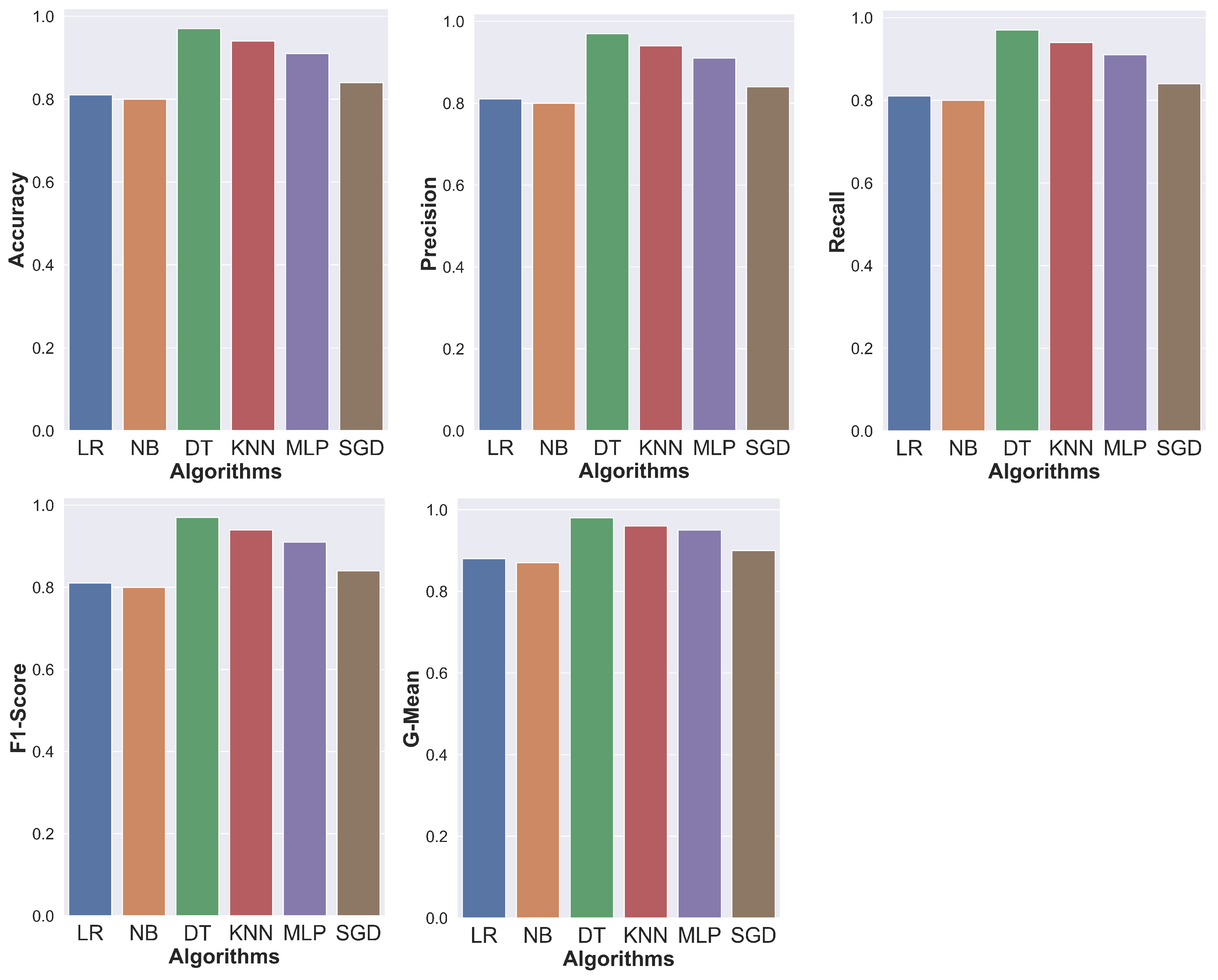
Table 2 illustrates the results obtained using the Udacity dataset for the main investigated classification algorithms. As observed from the results, the DT algorithm produced the best results when it was used to train a model. It achieves a G-Mean value of 98%, representing an excellent percentage of positive predictive values concerning all the predictive values. However, the results of the rest of the measures equal a percentage of 97%. Compared to the DT, the G-Mean of the KNN algorithm is 2% lower. We also note that the MLP comes third with good results after KNN; it has a 1% lower G-Mean value than the KNN with a value of 95% for the G-Mean measure. The MLP algorithm is followed by the SGD algorithm, which achieved 90% G-Mean, 5% lower than the MLP. The LR is 2% lower than the SGD; its score is 88% in G-Mean. Comparatively, the NB has the lowest score of all of the algorithms with 87% G-Mean and it achieves 80% at the rest of the measures.
Figure 7 shows a graphical representation of these measured measures: Accuracy, Precision, F1-Score, G-Mean, and Recall of all the algorithms for the Udacity dataset. It should be clearly noted from the figure that the DT algorithm is the best algorithm that obtained the highest accuracy. We can also rank the algorithms according to their performance for all the measures as DT, KNN, MLP, SGD, LR, and NB, where DT has the highest and NB has the lowest values.
5.2. Evaluation of Classification Algorithms on the BDD100K Dataset
The results we obtained using the BDD100K dataset are presented in
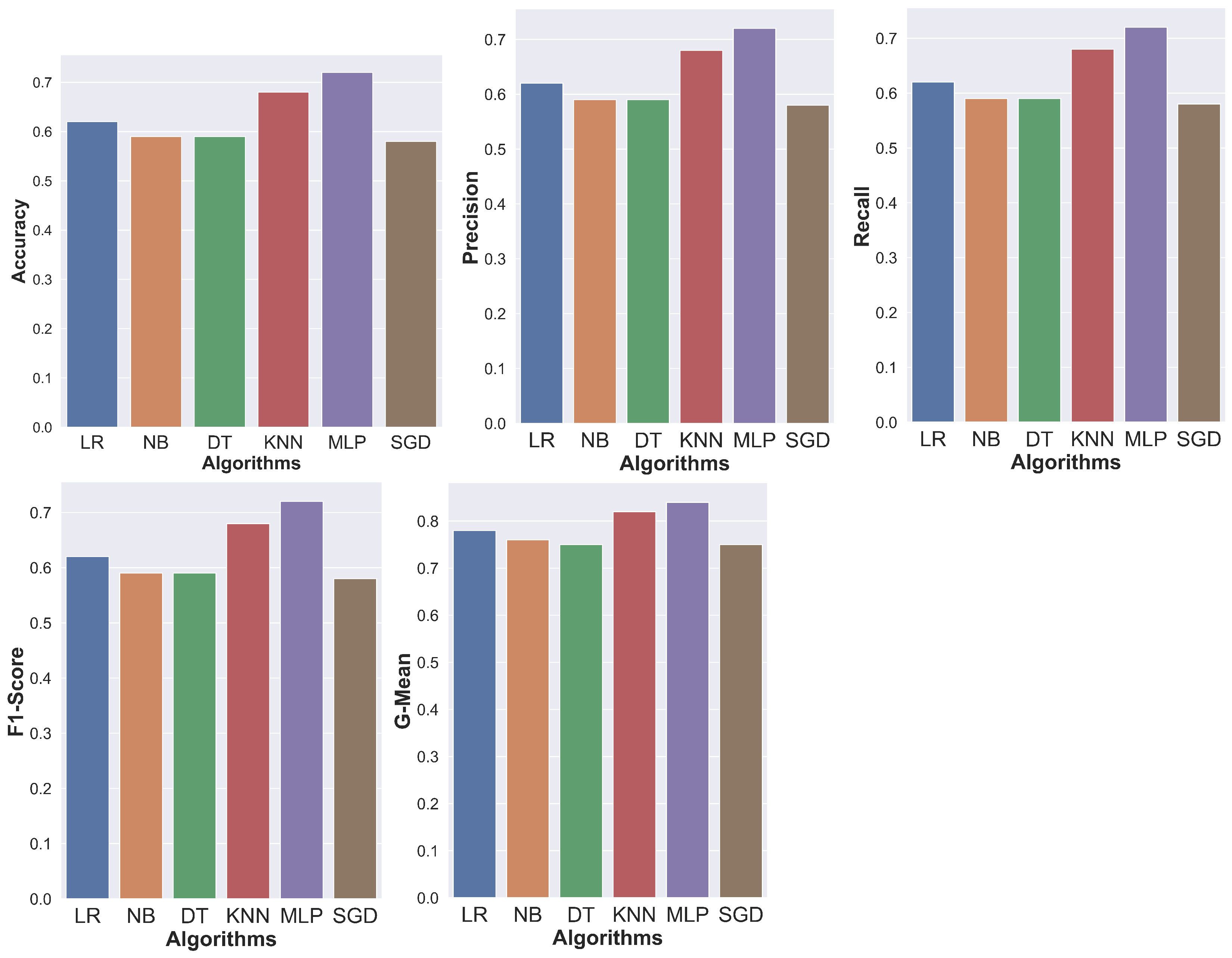
Table 3. MLP achieved the best results, with a G-Mean value of 84% (i.e., the best result among all measures for the same algorithm). This measure considers the balance between the classification performances of both the majority and minority classes. The results of the other measures are all equal, with a percentage of 72%. The KNN algorithm’s G-Mean measure is 2% lower than the MLP. Compared to other algorithms, the SGD and DT algorithms have the lowest G-Mean score of 75%. In contrast, the DT algorithm outperforms the SGD algorithm in all other measures by 1%, with an overall score of 59%.
Figure 8 graphically shows the score measures: Accuracy, Precision, F1-Score, G-Mean, and Recall of the tested algorithms for the BDD100K dataset. From the figure, it should be noted that the MLP Algorithm is the best that obtained the highest Accuracy. KNN followed by LR has the best G-Mean, which achieved 78% G-Mean, 4% lower than the KNN and 6% lower at the rest of the measures with a percentage of 62%. While NB is 2% lower than the LR, its score was 76% in the G-Mean and is 3% lower at the rest of the measures with a percentage of 59%.
5.3. Evaluation of the Grouped Dataset
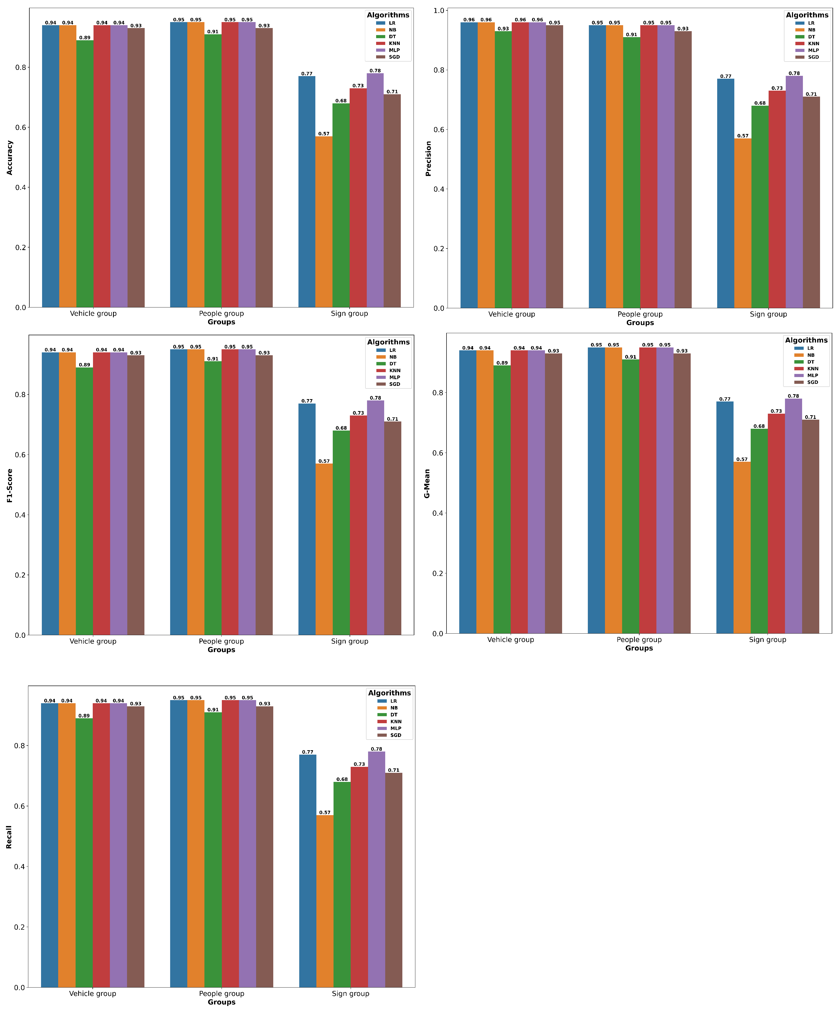
In this section, we evaluate the same measures on the grouped BDD100K dataset, displayed in
Table 4. The results here are much higher than those on the same ungrouped dataset. The LR, NB, KNN, and MLP are the best algorithms that obtained the highest score across all of the measures for the vehicle group. They scored 96% for G-Mean. These algorithms are followed by the SGD algorithm, which achieved 95% G-Mean, 1% lower than these algorithms. Comparatively, the DT algorithm has the lowest score of all of the algorithms, 2% lower than the SGD; its score was 93% in G-Mean. The other measures recorded a value of 94% for LR, NB, KNN, and MLP algorithms, a value of 89% for the DT, and a value of 93% for the SGD algorithm.
For the people group, the LR, NB, KNN, and MLP are the best algorithms that obtained the highest score across all measures. For the sign group, the MLP is the best algorithm that obtained the highest score across all of the measures; it scored 78% across all. The MLP was followed by the LR, which was 1% lower than the MLP algorithm. KNN is 5% lower than the MLP, its score was 73% across all of the measures.
Figure 9 illustrates score measures: Accuracy, Precision, F1-Score, G-Mean, and Recall of the tested algorithms for the obtained groups based on the nature (i.e., vehicles, people, and signs) from the BDD100K dataset. It is observed from the figure that the vehicle group gets the highest score in all measures. The results of the signs group were the worst among them.
5.4. Comparison Results
This section compares our obtained results to another recent comparable paper. It also compares the score for the BDD100k dataset overall classes with the scores from the modified grouped dataset.
The DT algorithm in our approach produced an Accuracy of 97%, while C. R. Kumar [
32] obtained 93%. We have also seen an increase in the Precision measure; we obtained 98% while they obtained 90%. Furthermore, the F1-Score and Recall were 97%, whereas the score for the other paper was 90%. We have achieved a higher percentage in Accuracy, Precision, F1-Score, and Recall measures compared to C. R. Kumar [
32]. This is justified by the fact that, when we cleaned the dataset, we combined all of the classes that fall under the umbrella of the traffic light categories into a single class that we have named “Traffic Light”.
Table 5 shows the comparison results between recent similar work and our contribution to the Udacity dataset.
Further, the test ranking for the Udacity dataset for the various classifiers is applied in
Table 6. It can be observed from the table that the DT has achieved the best rank for all the measures followed by KNN. In contrast, NB has the worst ranking compared to the other classifiers. The Friedman chi-square value based on the ranks equals 25.0 with a
p-value of 0.000139. Considering
, we can reject the null hypothesis indicating a significant difference between the various classifiers.
The second comparison is between the overall classes of the BDD100k dataset and the scores obtained after modifying the dataset by grouping similar categories into three main groups: vehicles, people, and signs. We got results that we compared with results obtained from the grouped dataset. After grouping the dataset, we saw an improvement in all of the measures adopted in our study. The following are our findings for the various measures we used: the MLP algorithm yielded the best results for G-Mean in BDD100K with an 84% score. In contrast, the best result we obtained from the group dataset of vehicles using the LR, NB, and KNN for G-Mean was 96%. The LR, NB, KNN, and MLP algorithms achieved the most outstanding results on all scales for 90% of the people group. The MLP algorithm achieved 78% on all measures for the group of signs, the highest score in the group. Except for the NB in the group of signs, all results in split groups were better than the overall results of the dataset. Here, we can state that collecting the original data into groups improved the prediction and classification results. This is the objective of our work by enhancing the performance of detecting the existing objects from the dataset used.
6. Conclusions and Future Work
This paper shows a comparison of machine learning algorithms. Six supervised learning algorithms are compared in this study. The datasets used in this research are Udacity and BDD100K. In the training step, we use 80% of the dataset to train each algorithm. Finally, methods are used to evaluate 20% of the datasets. The results show the decision tree we used produced a G-Mean of 98%, with the highest score in the Udacity dataset and the best score across all experiments. In contrast, the results obtained from the groups were better than the original dataset for the vehicles group using the LR, NB, and KNN with a G-Mean of 96%. The results of the algorithms were improved due to dividing the original dataset into groups, which, in turn, accomplishes the objective of our research, which is the increase in performance using our approach. The vehicle groupings come out on top with the highest score possible for this measure. The results for the signs group were the worst of all of them. However, except for the Precision measure, the remaining measures for the people group had the best results for all the groups. In the future, other studies might consider data classification according to the object’s size, speed, and whether it is moving or fixed. In addition, experiments can be conducted with other algorithms.


