Research on the SSIDM Modeling Mechanism for Equivalent Driver’s Behavior

Abstract

To solve the problem of smooth switching between the car-following model and lane-changing model, the Intelligent Driver Model (IDM) for a single lane was used to study the driver’s behavior switching mechanism of normally following, generating intentions to change lanes, creating space and speed gains, and performing lane change. In the case of sufficient lane-changing space and speed gains, the ego vehicle’s intention to change lanes was considered to solve the switching boundary between car-following behavior and lane-changing behavior, which is also the IDM failure point. In the event that there are no lane-changing gains, the IDM was optimized by incorporating the constraint components of the target lane vehicles in conjunction with the actual motion state of the ego vehicle, and the Stepless Switching Intelligent Driver Model (SSIDM) was constructed. Drivers’ natural driving information was collected, and scenario mining was performed on structured roads. On the basis of the collected data, an elliptic equation was used to fit the behavior switching boundary, and the two component balance coefficients of the front and rear vehicles on the target lane were identified. According to the test set verification results, the Mean Square Error (MSE) of the SSIDM is 2.172, which is 57.98% less than that of the conventional single-lane IDM. The SSIDM can accomplish stepless switching comparable to the driver’s behavior between the car-following behavior and the lane-changing behavior, with greater precision than IDM. This research can provide theoretical support for the construction of the point-to-point driving model and the development of L2+ autonomous driving functions. It can provide assistance for the landing and application of full-behavior and full-scene autonomous driving.

1. Introduction

In recent years, with the rapid development of Internet of Vehicles (IoV) technology, various full-scene intelligent driving schemes supporting the integration of driving and parking, such as Navigate on Pilot (NOP) and Navigate on Autopilot (NOA), have begun to be deployed in mass-produced vehicles [1]. Car-following behavior and lane-changing behavior are the two most fundamental driving behaviors for point-to-point driving [2]. In conjunction with the motion state of ego vehicle and surrounding interactive vehicles, it is necessary to frequently switch between the two categories of behavior. By studying the behavior switching mechanism from the driver’s perspective, solving the switching boundary, and considering the vehicle constraints of the target lane for equivalent modeling, it is possible to achieve stepless switching between car-following behavior and lane-changing behavior, which has important theoretical significance and practical value for building point-to-point full scene intelligent driving.

The majority of car-following models are based on theory and are rule-driven. IDM is the most popular and most accurate prediction method [3,4]. In 2000, Treiber M et al. [5] investigated the car-following behavior and proposed the IDM based on the influence of following distance and anticipated speed. Since then, specialists and academics have analyzed and optimized IDM from a variety of perspectives. Péter T et al. [6] conducted a detailed study on the mathematical description of the universal IDM, which takes into account the dynamic variations in the state characteristics of traffic processes. Qin P et al. [7] optimized the applicable boundary of IDM based on road geometric conditions such as camber, superelevation, and slope. Yi Z et al. [8] developed the Intelligent Back-looking Distance Driver Model (IBDM) with the influence of rear vehicles in the same lane. The Autonomous Vehicle-Intelligent Driver Model (AV-IDM) was created by Sharath M. and his team while taking into account circumferential environmental vehicles [9]. Li Y et al. [10] established a Long Short Term Memory-Intelligent Driver Model (LSTM-IDM) governed by data rules capable of simulating extreme vehicle conditions such as static or extreme acceleration. Yang L. et al. [11] added a cognitive risk coefficient to IDM based on driver behavior in ice and snow conditions and validated the model’s efficacy and robustness. Jin P. et al. [12] delved into the impact of data error accumulation on IDM precision and developed an error calibration function to reduce cumulative error. A hybrid flow simulation model, which merges IDM and Cooperative Adaptive Cruise Control (CACC), was developed by Chang X et al. [13] in their study. The model’s effectiveness was verified by its simulation of heterogeneous traffic flow. Hu X et al. [14] established PS-IDM on the basis of IDM considering the change in the driver’s psychological state caused by the invasion of other vehicles and demonstrated that PS-IDM can improve car-following performance effectively. Péter T et al. [15] applied the reduced network traffic model to the IDM and verified the optimization on the open road. Bouadi M et al. [16] studied the influences of stochastic factors on the car-following model, and Stochastic Intelligent Driver Model (SIDM) was established considering both the inter-vehicular gap and the velocity difference. In addition to the optimization of the IDM model, Wang Z et al. [17] proposed an algebraic framework that does not involve parameter optimization identification for evaluating and comparing car-following models with linearly identifiable parameters. A data-driven car-following model was established by Qu D et al. [18], based on CNN-BiLSTM-Attention for CAV, which has high accuracy in vehicle-trajectory prediction.

The lane-changing intention is caused by the driver’s dissatisfaction with the current driving state causes, which compels the driver to generate space and speed gains prior to changing lanes through acceleration and deceleration in a specific time domain. Yuan W et al. [19] defined eye movement parameters such as fixation time and saccade amplitude to effectively recognize a driver’s lane-changing intention from the perspective of the driver’s physiological characteristics. From the standpoint of the vehicle’s motion state, there are currently two methodologies for lane-changing intention recognition of rule-driven and data-driven [20]. In terms of rule-driven, Zhu N. et al. [21] constructed dynamic and static risk fields based on the theory of artificial potential fields and characterized the lane-changing risk by defining driver lane-changing planning and safety threshold. Chen H. et al. [22] developed a dissatisfaction accumulation model based on the driver’s anticipated speed in order to evaluate lane-changing decisions. Wang J. et al. [23] introduced two quantitative indicators of lane-changing intensity and risk factors to devise and identify safe lane-changing conditions. Using the relative motion state of the ego vehicle and the surrounding vehicles, Ji X et al. [24] established a data-driven LSTM model for recognizing the driver’s lane-changing intention. Guo Y. et al. [25] developed a model for the recognition of lane-changing intentions based on the LSTM model of the attention mechanism. Zhao J. et al. [26] proposed a recognition model of lane-changing intention that utilized a combination of the convolutional neural network, gated recurrent neural network, and transformer model.

There were also many behavioral analysis studies directly related to driver style. In terms of car-following behavior, Makridis M. et al. [27] proposed a new modeling method of car-following behavior, in which the characteristics of the driver and vehicle were taken as input. The Microsimulation Free-flow aCceleration (MFC) model was used to clearly reproduce the influence of vehicle dynamics and driver behavior. Adavikottu A. et al. [28] studied the driving behavior of aggressive drivers, which tends to be closer car-following distance, smaller TTC, rapid acceleration, and rapid deceleration. The results can be used to guide the construction of the car-following model for differentiated drivers. In terms of lane-changing behavior, Antin J. et al. [29] investigated the real lane-changing behavior combined with natural driving data, and it was found that elderly drivers may not be able to perform shoulder saccades before lane-changing behavior, resulting in a greater error rate. Li X. et al. [30] found that it was helpful to understand the driver’s interaction tendency to study the different attitudes of different drivers to FAVS lane-changing behavior according to their age, gender, and driving experience. These kinds of research have studied the real car-following behavior and lane-changing behavior of drivers with different styles but have not considered the switching mechanism of car-following behavior and lane-changing behavior.

Presently, the majority of car-following models and lane-changing intention recognition models are independent of each other. The switching between car-following behavior and lane-changing behavior is a stepped switching across models, which results in poor smoothness and stability of switching during simulations or real-vehicle verifications. This paper combined the entire process of behavior switching from the normal following, the generation of lane-changing intention, the creation of lane-changing space and speed gains, and the execution of lane change. Taking the scenario of changing lanes after following a large vehicle for a distance as an example, the IDM was calibrated using natural driving data, and the switching boundary was determined. The target lane vehicle constraint components were added to construct SSIDM based on the switching boundary, and the balance coefficients of SSIDM were determined by actual data. On the basis of the test set, the model’s predictive accuracy was validated. The results demonstrate that the model can realize the car-following behavior to lane-changing behavior stepless switching equivalent to the driver’s coherent driving behavior, and that the model’s accuracy is high, which is crucial for the realization of point-to-point full scene intelligent driving simulation.

2. Behavior Switching Scenario Mining

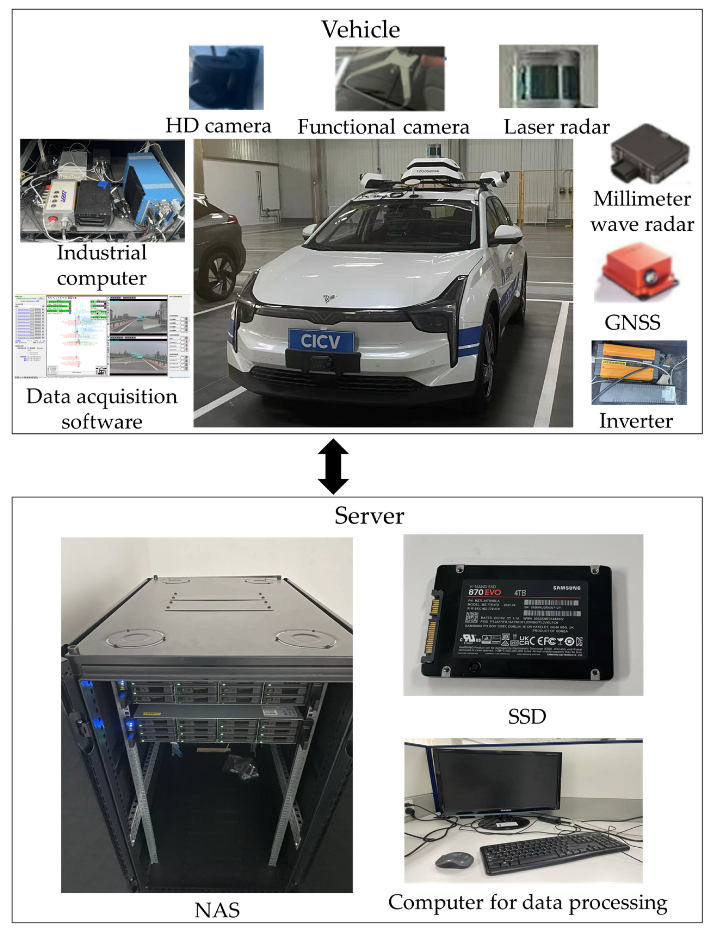
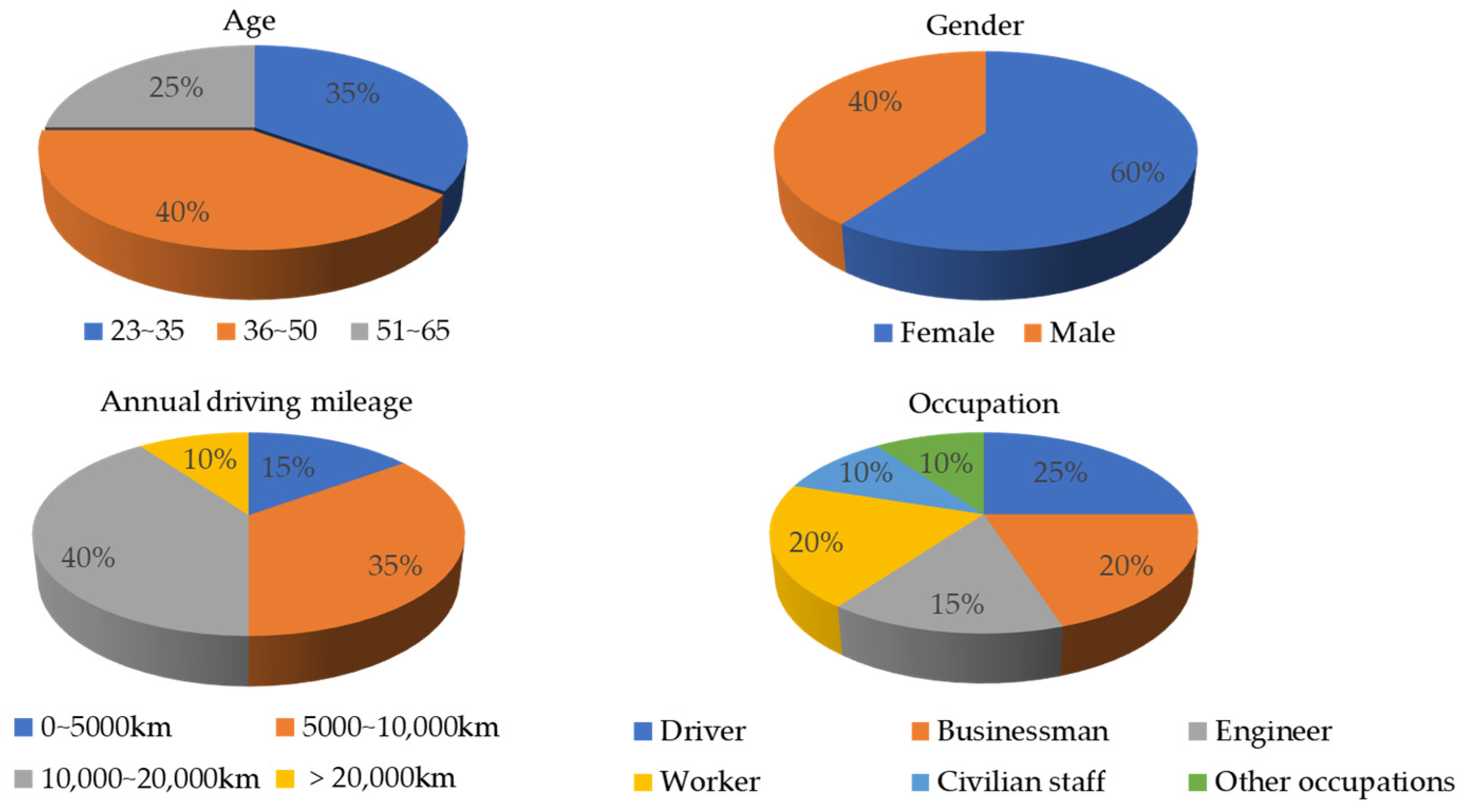
2.1. Natural Driving Data Collection

A data acquisition system was designed to collect information about the driver’s natural driving behavior on open roads. As the test vehicle, an electric vehicle was equipped with functional cameras, millimeter-wave radars, lidars, GNSS and HD cameras. The information on the circumferential targets was obtained by the target-level data fusion of the functional cameras and the radars. The positioning, heading angle, road curvature, and other information of the test vehicle were collected by GNSS. The high-performance industrial computer was connected to various sensors to obtain text and video data in real-time. Concurrently, Network Attached Storage (NAS) equipment was deployed on the vehicle and office terminals to accomplish large-capacity storage, which communicated with industrial computers via high-speed network interfaces. The entire system is shown in Figure 1.

A total of 20 experienced drivers were recruited to execute driving tasks, and the information about the drivers’ age, gender, annual driving mileage, and occupation are shown in Figure 2. The majority of the collection was structured roads, including highways and urban expressways.

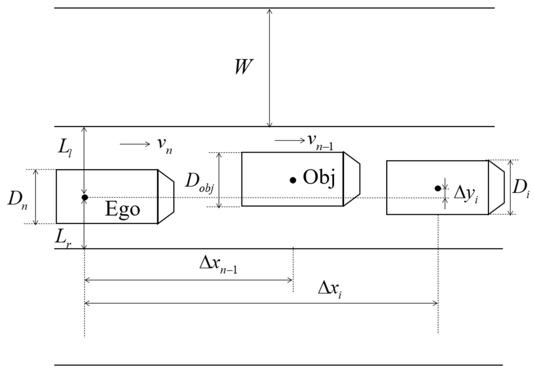
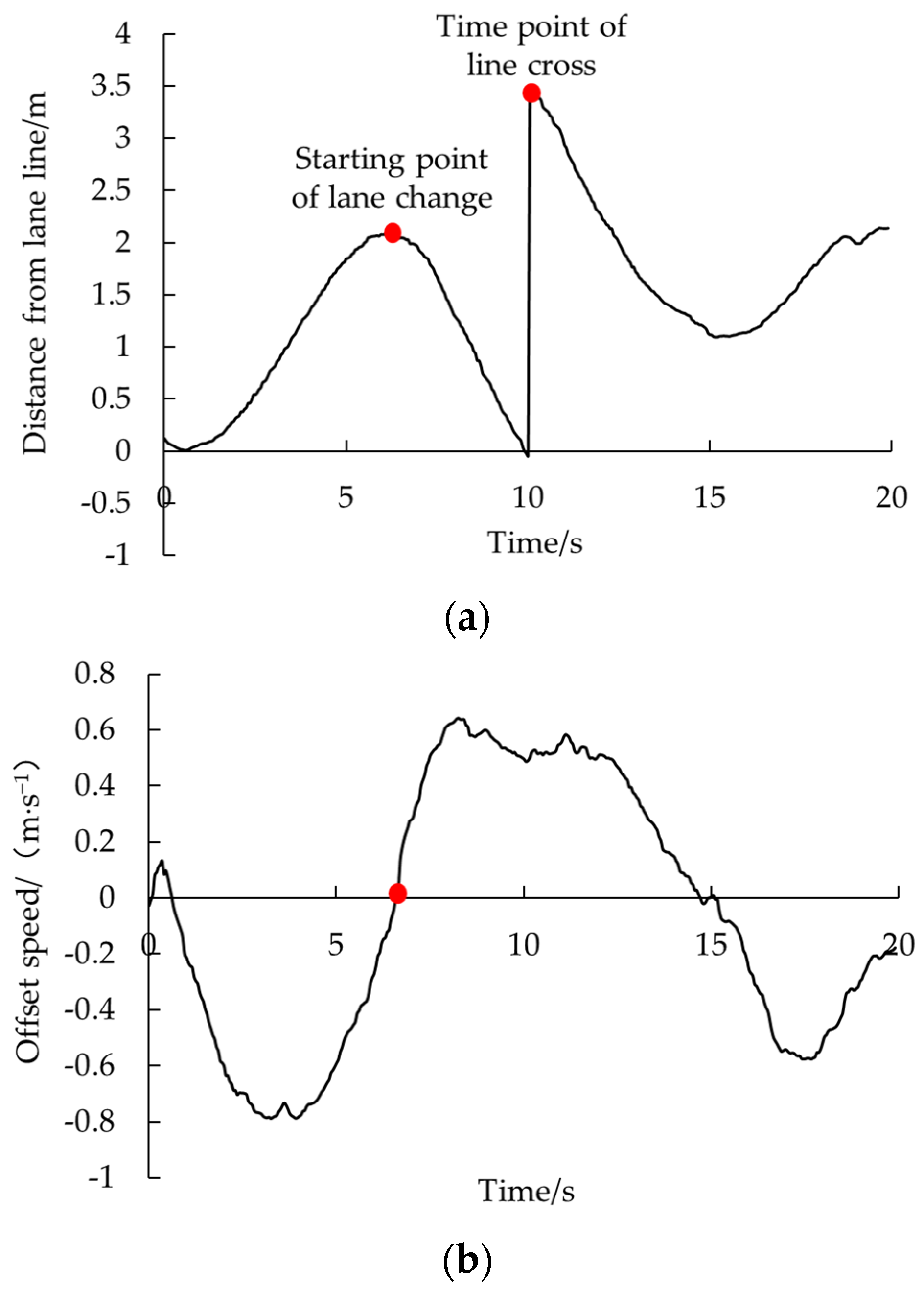
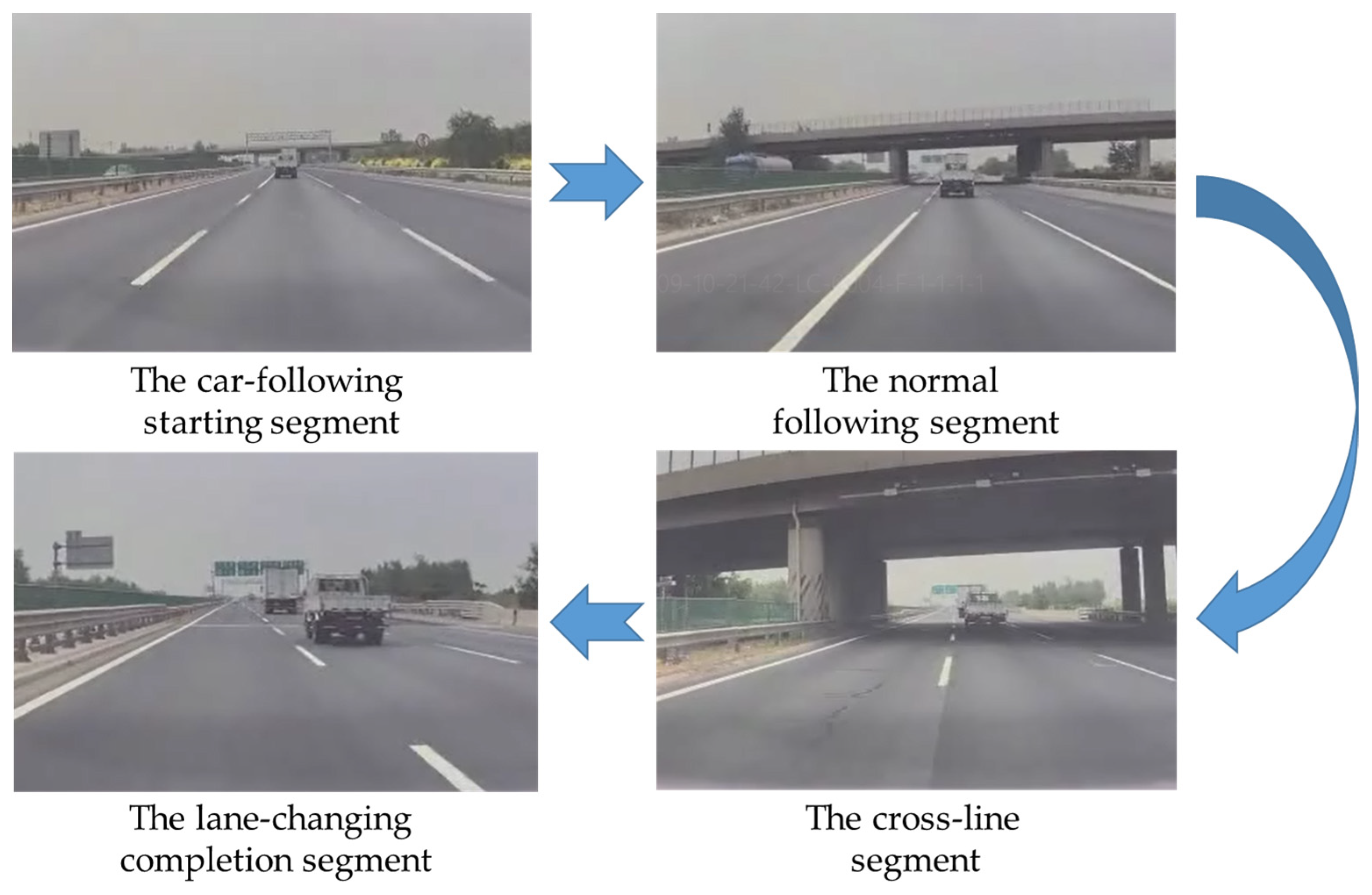
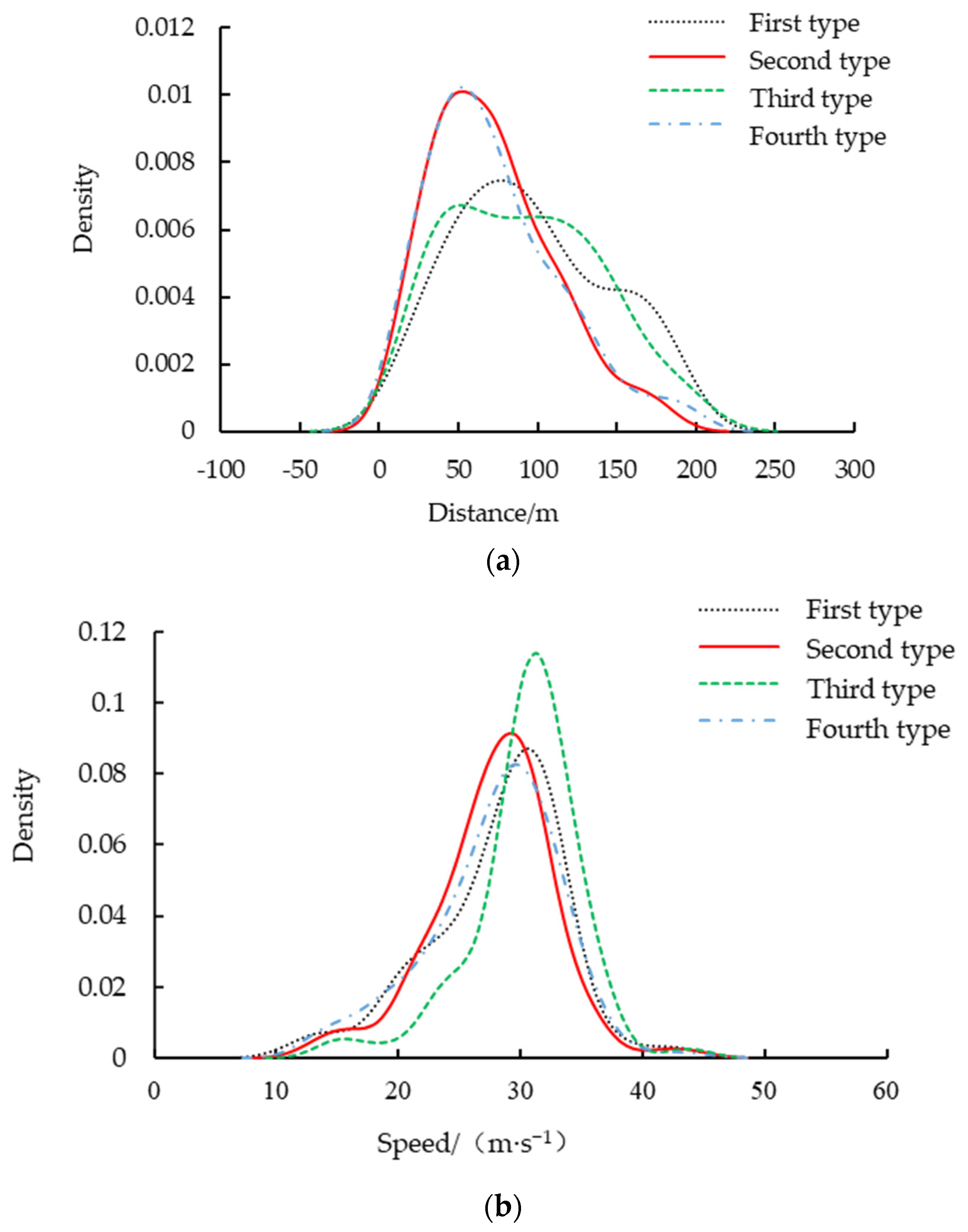
2.2. Behavior Scenario Mining

After cleaning multi-source heterogeneous original data, car-following behavior to lane-changing behavior scenario mining was performed. Initially, the switching behavior was defined, which included the car-following starting segment, the normal following segment, the cross-line segment, and the lane-changing completion segment. Among them, the starting segment of the car-following behavior was defined as the constraints between the ego vehicle and the front vehicle in the ego lane. For clear expression constraints, Figure 3 is shown as follows.

Figure 3 includes the distance constraint between the ego vehicle and the lane line, the speed constraint of the ego vehicle, the distance constraint between the front vehicle and the lane line, the distance constraint between the front vehicle and the ego vehicle, and the speed constraint of the front vehicle. The origin of the coordinates was defined as the center of the ego vehicle rear axle. The specific constraints are as follows.

$$\{\begin{array}{l}\frac{D_n}{2}<L_l<W-\frac{D_n}{2}\cup \frac{D_n}{2}<L_r<W-\frac{D_n}{2}\\ v_n>0\\ L_r-\left|\mathsf{\Delta }{y}_i\right|-\frac{D_i}{2}>0\cup L_l-\left|\mathsf{\Delta }{y}_i\right|-\frac{D_i}{2}>0(i=1,2\dots n)\\ \mathsf{\Delta }{x}_{n-1}=\min \mathsf{\Delta }{x}_i(i=1,2\dots n)\\ \mathsf{\Delta }{x}_{\min }\le \mathsf{\Delta }{x}_{n-1}\le \mathsf{\Delta }{x}_{\max }\\ v_{n-1}>0\end{array}$$

(1)

where D_n is the width of the ego vehicle, W is lane width, L_l and L_r are the distance from the coordinate origin to the left and right lane lines, v_n is the ego vehicle speed, D_i is the width of each vehicle identified in the ego lane, $\mathsf{\Delta }{x}_i$ and $\mathsf{\Delta }{y}_i$ are the relative longitudinal and lateral distances between each vehicle identified in the ego lane and the ego vehicle, $\mathsf{\Delta }{x}_{n-1}$ is the relative longitudinal distance of the following target, $\mathsf{\Delta }{x}_{\max }$ and $\mathsf{\Delta }{x}_{\min }$ are the relative longitudinal distance thresholds between the ego vehicle and the following target, $v_{n-1}$ is the following target speed.

The normal following segment was defined as the distance without mutation between the ego vehicle and the following target on the basis of satisfying the above conditions. All types of cut out and cut in scenarios were filtered out. The limitation is as follows:

$$|\mathsf{\Delta }{x}_{n-1}(t)-\mathsf{\Delta }{x}_{n-1}(t-1)|<\mathsf{\Delta }{x}_s$$

(2)

where $\mathsf{\Delta }{x}_s$ is the distance mutation threshold.

The cross-line segment was based on the lane line with the maximum level of confidence, which was defined as beginning to shift to the lane line on the lane-changing side until the distance changed abruptly. The distance from the lane line is shown in Figure 4a. As shown in Figure 4b, the starting point of lane change was determined by the speed of the offset lane line, with the zero point of the offset speed change serving as the starting point.

Taking the steering wheel angle threshold and the distance threshold between the ego vehicle and the lane line as constraints, the constraints are as follows:

$$\{\begin{array}{l}|L_l(t)-L_l(t-1)|>L_{\min }\\ |\delta (t)|>{\delta }_{\min }\end{array}$$

(3)

where $\delta$ is the steering wheel angle, $L_{\min }$ and ${\delta }_{\min }$ are the lane line distance mutation threshold and the steering wheel angle threshold, respectively.

The lane-changing completion segment was defined by the vehicle’s stable driving in the target lane after crossing the line, and the comprehensive judgment was based on the yaw angle and steering wheel angle of the ego vehicle. When following large vehicles, drivers have a greater incentive to change lanes due to the safety principle. To eliminate the effect of the front vehicle type on the intention to change lanes, the variable was unified and the target type in front was restricted to large vehicles. Considering that the left lane is generally a fast lane, the left lane-changing scenario was finally selected. Figure 5 depicts the mined scenario.

3. IDM Parameter Identification

3.1. IDM Modeling Mechanism

On the basis of the generalized force model, IDM for single lane car-following behavior was proposed. The research focused on alterations in traffic flow. It is capable of simulating the transition from free flow to congested flow, accounting for the acceleration trend in the free state of the vehicle and averting the deceleration trend of the front vehicle collision. It belongs to the expected measurement model and the specific expression is as follows:

$$\{\begin{array}{l}\frac{d{v}_n(t)}{dt}=a[1-{(\frac{v_n(t)}{\tilde{v}})}^{\sigma }-{(\frac{S^{*}(v_n(t),\mathsf{\Delta }{v}_{n-1}(t))}{\mathsf{\Delta }{x}_{n-1}(t)})}^2]\\ S^{*}(v_n(t),\mathsf{\Delta }{v}_{n-1}(t))=\tilde{s}+\tau v_n(t)+\frac{v_n(t)\mathsf{\Delta }{v}_{n-1}(t)}{2\sqrt{ab}}\end{array}$$

(4)

where $\tilde{v}$ is the driver’s expected speed, $\sigma$ is the acceleration index, $a$ is the maximum acceleration of the ego vehicle, $b$ is the comfortable acceleration of the ego vehicle, $\tilde{s}$ is the blocking interval, $\tau$ is the expected headway, $\mathsf{\Delta }{v}_{n-1}(t)$ is the relative speed of the ego vehicle and the front vehicle.

IDM can simulate the acceleration trend in a free flow. At this time, Δx(t) approaches infinity, and the IDM can be rewritten as follows:

$$\frac{d{v}_n(t)}{dt}=a[1-{(\frac{v_n(t)}{\tilde{v}})}^{\sigma }]$$

(5)

In a congested flow state, the model can also be used to simulate the braking trend of the ego vehicle. At this time, the IDM can be simplified as follows.

$$\frac{d{v}_n(t)}{dt}=-a[{(\frac{S^{*}(v_n(t),\mathsf{\Delta }{v}_n(t))}{\mathsf{\Delta }x(t)})}^2]$$

(6)

3.2. Model Parameter Identification

Based on the Genetic Algorithm (GA) and actual data, IDM identification parameters were calibrated. GA is a random global search optimization method which starts from any initial population. Through selection, crossover and mutation operations, a group of individuals are generated which are more suitable for the environment, so that the group evolves to a better and better area in the search space. In this way, the generation continues to reproduce and evolve, and eventually converges to a group of individuals most suitable for the environment, resulting in a high-quality solution to the problem. GA has good versatility, a wide range of application scenarios, and minimal application restrictions. It has been proven to achieve an excellent optimization effect. At the same time, GA originates from the solution set and has a larger coverage, which is more conducive to the global preferred orientation. As the objective function, the Root Mean Square Percentage Errors (RMSPE) were introduced. The predicted values and actual values of relative speed and relative distance were compared. The objective function is described as follows.

$$S_{RMSPE}=\sqrt{\frac{1}{n}{\displaystyle \sum _{t=1}^n\frac{{(\mathsf{\Delta }{x}_{n-1}(t)-\widetilde{\mathsf{\Delta }{x}_{n-1}}(t))}^2}{{(\mathsf{\Delta }{x}_{n-1}(t))}^2}}}+\sqrt{\frac{1}{n}{\displaystyle \sum _{t=1}^n\frac{{(v_n(t)-\widetilde{v_n}(t))}^2}{{(v_n(t))}^2}}}$$

(7)

where n is the total number of samples, $\widetilde{\mathsf{\Delta }{x}_{n-1}}$ is the predicted relative distance between the two vehicles and $\widetilde{v_n}$ is the predicted ego vehicle speed.

The initial population was set to 100, and its population of individuals was determined by a roulette wheel. The crossover operator was defined as a uniform crossover, and the crossover probability was 0.8. The mutation operator was defined as a uniform mutation, and the mutation probability was 0.1. The training set and test set were divided by 7:3 based on the typical car-following segment data. The parameter identification results are shown in

Table 1. IDM identification results.

Parameter	$\tilde{\mathit{v}}$/(m·s−1)	$\mathit{\sigma }$	$\mathit{a}$/(m·s−2)	$\mathit{b}$/(m·s−2)	$\tilde{\mathit{s}}$/m	$\mathit{\tau }$/s
Value	35.022	0.018	0.218	1.503	13.262	2.606

.

The identification results were verified based on the test set, and MSE was used to evaluate the speed prediction results of the ego vehicle. The comparison between the actual speed of the ego vehicle and the speed predicted by IDM is shown in Figure 6.

The calculated MSE value for the test set was 0.749, representing an accurate identification result. For the behavior of following large vehicles, these identification results can be used to predict the motion state of the ego vehicle.

4. Construction of SSIDM

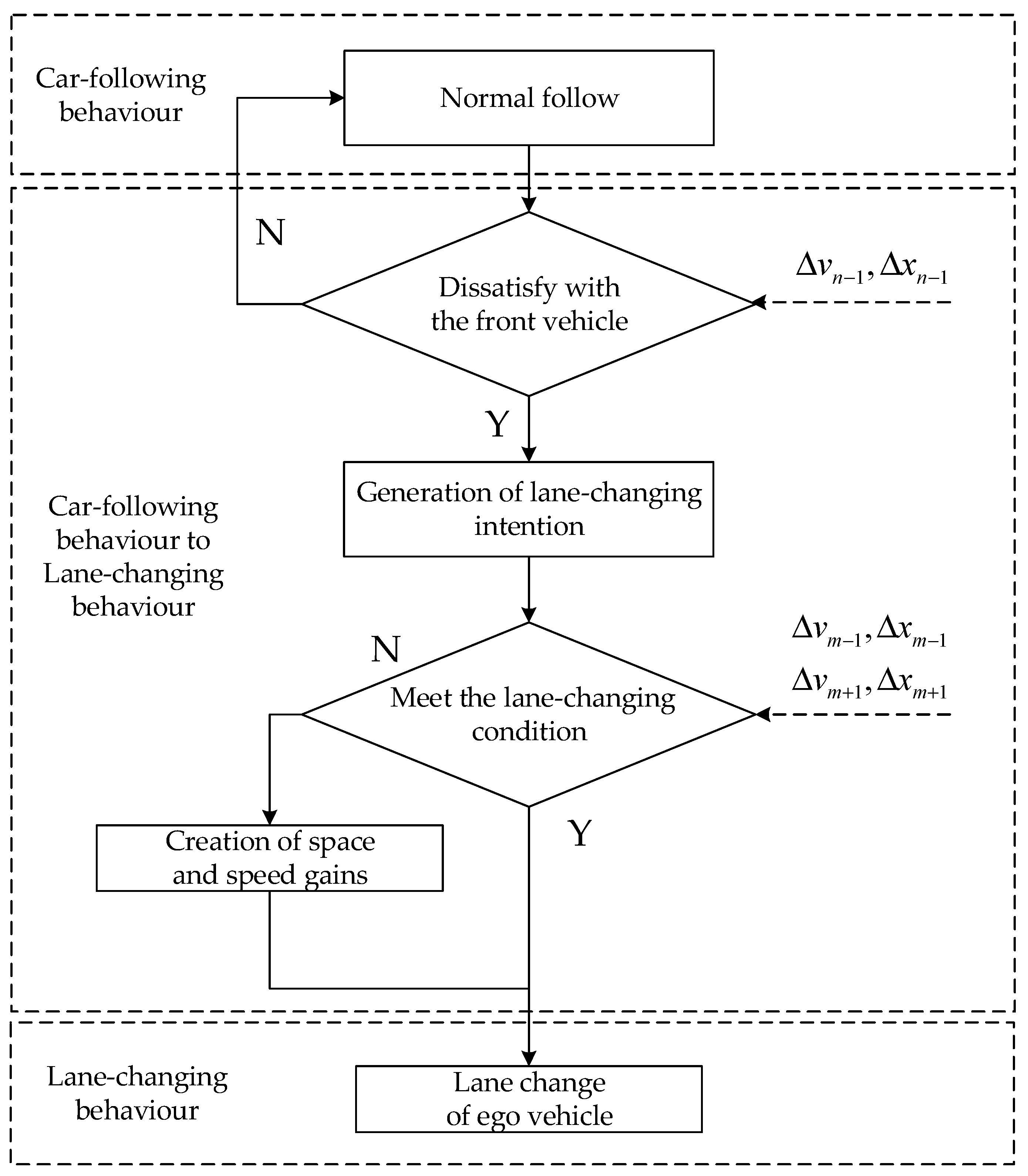
4.1. Modeling Mechanism of SSIDM

IDM is proposed for car-following behavior in a single lane. In a broad sense, it is expressed that the vehicle will accelerate when it is far away from the front vehicle and decelerate when it is close to the front vehicle. However, in the actual car-following process, due to the dissatisfaction with the relative distance or speed of the front vehicle, the driver of the ego vehicle will produce the intention of changing lanes, and the decision is made through lane selection and whether to change lane. If the target lane has enough space and speed gains, the driver of the ego vehicle will immediately change lanes, and the relative motion state between the ego vehicle and the front vehicle is defined as the switching boundary. If the target lane has front and rear vehicle constraints, the driver of the ego vehicle will change the motion state to create space and speed gains. This behavior still belongs to the car-following model, but the influence of the target lane vehicles needs to be considered on the basis of the single lane IDM. The relative distances between the vehicle and the front and rear vehicles of the target lane were defined as $\mathsf{\Delta }{x}_{m-1}$ and $\mathsf{\Delta }{x}_{m+1}$, and the relative speeds between the vehicle and the front and rear vehicles of the target lane were defined as $\mathsf{\Delta }{v}_{m-1}$ and $\mathsf{\Delta }{v}_{m+1}$. The SSIDM modeling mechanism for car-following behavior to lane-changing behavior switching is shown in Figure 7.

Based on whether the target lane has constrained vehicles, all segments were divided into four categories: only affected by the front vehicle of the ego lane, affected by the front vehicle of the ego lane and the front vehicle of the target lane, affected by the front vehicle of the ego lane and the rear vehicle of the target lane, affected by the front vehicle of the ego lane and the front and rear vehicles of the target lane. In order to characterize the differences in behavior switching boundary, four types of scenarios were analyzed, and the independence between variables was considered. Finally, the speed of the ego vehicle, the relative distance from the front vehicle, and the speed of the front vehicle were taken as the characteristic parameters to obtain the statistics of the key parameters of the lane-changing starting point for each type of scenario. The statistical results are shown in

Table 2. Statistical results.

Statistic		Mean Value	Standard Deviation
First type	$v_n$/(m·s−1)	28.108	5.491
	$\mathsf{\Delta }{x}_{n-1}$/m	95.569	48.412
	$v_{n-1}$/(m·s−1)	21.602	3.915
Second type	$v_n$/(m·s−1)	27.788	4.879
	$\mathsf{\Delta }{x}_{n-1}$/m	71.472	38.233
	$v_{n-1}$/(m·s−1)	20.998	3.697
Third type	$v_n$/(m·s−1)	30.424	4.426
	$\mathsf{\Delta }{x}_{n-1}$/m	91.829	47.457
	$v_{n-1}$/(m·s−1)	21.209	3.581
Fourth type	$v_n$/(m·s−1)	27.811	5.393
	$\mathsf{\Delta }{x}_{n-1}$/m	72.232	41.618
	$v_{n-1}$/(m·s−1)	21.178	3.763

.

To analyze the characteristics of the parameters, the kernel density estimation of these three types of parameters was carried out. The kernel density curves corresponding to the speed of the ego vehicle, the relative distance from the front vehicle, and the speed of the front vehicle are shown in Figure 8.

Through the analysis of the statistical table and the kernel density estimation curves, it can be concluded that for the second and fourth types of scenarios, the relative distance between the ego vehicle and the followed front vehicle is the closest as shown in Figure 8a. Due to the influence of the front vehicle in the target line, it is necessary to leave enough space when performing lane change. For the third type of scenario, the ego vehicle speed is the largest as shown in Figure 8b. Since there is a rear vehicle in the target lane in the third type of scenario, the ego vehicle needs to accelerate to exceed the vehicle in the target lane to create lane-changing space. The speeds of the followed vehicles in the four scenarios are basically consistent and concentrated as shown in Figure 8c. The ego vehicle speed was defined as the input independent variable, and it can be judged that the ego vehicle speed at the initial point of lane change is mainly affected by the relative distance from the front vehicle in these four scenarios. The relationship between the ego vehicle speed and the relative distance of the front vehicle in four scenarios is shown in Figure 9.

According to the distribution of Figure 9, it can be seen that in the four types of scenarios, the ego vehicle speed is positively correlated with the relative distance between the two vehicles, and the slope gradually increases, which is in compliance with the principle of car-following safety. At the same time, when the speed of the ego vehicle exceeds 30 m·s⁻¹, the car-following distance exceeds 150 m, which is separated from the car-following relationship and is also consistent with the actual high-speed driving situation.

4.2. Solution of Switching Boundary Conditions

Considering that the drivers’ response time is short, if the target lane has no front and rear vehicle constraints, the lane change will be carried out immediately when the tolerance boundary is reached. Therefore, the initial point of lane change in the first type of scenario can be directly defined as the drivers’ tolerance boundary. The scatter distribution of the relative distance between the ego vehicle and the target vehicle in the first type of scenario is shown in Figure 10.

It can be seen from Figure 8 that the shape of the scatter distribution is approximately to the convex function, so various commonly convex functions were used for fitting. Based on GA, the fitting parameters were optimized and evaluated by goodness of fitting. The identification evaluation results are shown in

Table 3. Fitting evaluation results.

Fitting Function		Value	R2
$\mathsf{\Delta }{x}_{n-1}=k{(v_n)}^a+b$	k	6.2 × 10−3	0.473
	a	2.723
	b	26.281
$\mathsf{\Delta }{x}_{n-1}=k{a}^{v_n}+b$	k	6.841	0.401
	a	1.089
	b	1.837
$\mathsf{\Delta }{x}_{n-1}=d-\sqrt{c^2[(1-\frac{{(v_n-a)}^2}{b^2})]}$	a	0.315	0.572
	b	34.879
	c	180.245
	d	197.179
$\mathsf{\Delta }{x}_{n-1}={\displaystyle \sum _{i=0}^n{a}_i{v_n}^i}$	n	2	0.431
	a0	37.309
	a1	−3.589
	a2	0.198

.

By analyzing Table 3, the elliptic curve has the highest goodness of fitting, so the elliptic equation was finally selected to characterize the tolerance boundary conditions. The fitting results are shown in Figure 11.

This switching boundary can constrain the car-following behavior of large vehicles in front of the ego vehicle. When there are no interacting vehicles in the target lane, the relative distance from the front vehicle of ego lane reaches this switching boundary, the ego vehicle changes lanes, and the IDM fails.

4.3. Model Unified Expression

In the second, third, and fourth types of scenarios, if the switching boundary is reached but there is no lane-changing space or speed gains, the driver will change the motion state of the ego vehicle to generate lane change gains. Referring to the statistical distribution and kernel density estimation of the characteristic parameters of the four types of scenarios, a deceleration component was defined for the front vehicle of the target lane to ensure that the vehicle has sufficient lane change gains.

$$\{\begin{array}{l}△a_{m-1}^{-}={(\frac{S_{m-1}^{*}(v_n(t),\mathsf{\Delta }{v}_{m-1}(t))}{\mathsf{\Delta }{x}_{m-1}(t)})}^2\\ S_{m-1}^{*}(v_n(t),\mathsf{\Delta }{v}_{m-1}(t))=\tilde{s}+\tau v_n(t)+\frac{v_n(t)\mathsf{\Delta }{v}_{m-1}(t)}{2\sqrt{ab}}\end{array}$$

(8)

For the rear vehicle of the target lane, an acceleration component was defined to ensure that the vehicle has enough lane-changing space.

$$\{\begin{array}{l}△a_{m+1}^{+}={(\frac{S_{m+1}^{*}(v_n(t),\mathsf{\Delta }{v}_{m+1}(t))}{\mathsf{\Delta }{x}_{m+1}(t)})}^2\\ S_{m+1}^{*}(v_n(t),\mathsf{\Delta }{v}_{m+1}(t))=\tilde{s}+\tau v_n(t)+\frac{v_n(t)\mathsf{\Delta }{v}_{m+1}(t)}{2\sqrt{ab}}\end{array}$$

(9)

On the basis of IDM, the front and rear vehicle constraint components of the target lane were added. Considering the influence degree of the target lane vehicles on the ego vehicle, the dimensionless balance coefficients were added before the two components, and the vehicle acceleration can be obtained as follows:

$$\frac{d{v}_n(t)}{dt}=a[1-{(\frac{v_n(t)}{\tilde{v}})}^{\sigma }-{(\frac{S^{*}(v_n(t),\mathsf{\Delta }{v}_n(t))}{\mathsf{\Delta }{x}_{n-1}(t)})}^2-{\omega }_{m-1}△a_{m-1}^{-}+{\omega }_{m+1}△a_{m+1}^{+}]$$

(10)

where ${\omega }_{m-1}$ and ${\omega }_{m+1}$ are the balance coefficients of the front and rear vehicle components of the target lane, respectively.

When there is a certain lane-changing space and speed gains, the driver of the ego vehicle begins to change the lane. It is defined that there is enough lane-changing space when the front and rear vehicles of the target lane meet the safety distance and the distance between the front vehicle of the target lane and the ego vehicle is greater than the distance between the front vehicle of the ego line and the ego vehicle, and there are enough speed gains when the speed of the front vehicle of the target lane is greater than the speed of the front vehicle of the ego lane. This termination condition is used as the initial point of lane change in the second, third and fourth types of scenarios:

$$\{\begin{array}{l}|\mathsf{\Delta }{x}_{m+1}(t)|>\mathsf{\Delta }{x}_{safe}\cap \mathsf{\Delta }{x}_{m-1}(t)>\mathsf{\Delta }{x}_{safe}\\ \mathsf{\Delta }{x}_{m-1}(t)\ge \mathsf{\Delta }{x}_{n-1}(t)\\ \mathsf{\Delta }{v}_{m-1}(t)>\mathsf{\Delta }{v}_{n-1}(t)\end{array}$$

(11)

where $\mathsf{\Delta }{x}_{safe}$ is the safety distance threshold between the interactive vehicles in the target lane and the ego vehicle.

Finally, the complete SSIDM expression considering the front and rear vehicle constraints of the target lane can be obtained.

(1)

When the target lane has no front and rear vehicle constraints.

$$\{\begin{array}{l}\mathsf{\Delta }{x}_{n-1}(t)\ge d-\sqrt{c^2[(1-\frac{{(v_n(t)-a)}^2}{b^2})]}:\begin{array}{ccc}& & \begin{array}{ccc}& \begin{array}{cc}\begin{array}{cc}& \end{array}& \end{array}& (12\mathrm{a})\end{array}\end{array}\\ \frac{d{v}_n(t)}{dt}=a[1-{(\frac{v_n(t)}{\tilde{v}})}^{\sigma }-{(\frac{S^{*}(v_n(t),\mathsf{\Delta }{v}_n(t))}{\mathsf{\Delta }{x}_{n-1}(t)})}^2]\\ \mathsf{\Delta }{x}_{n-1}(t)<d-\sqrt{c^2[(1-\frac{{(v_n(t)-a)}^2}{b^2})]}:\begin{array}{cc}\begin{array}{cc}\begin{array}{cc}\begin{array}{cc}\begin{array}{cc}\begin{array}{cc}& \end{array}& \end{array}& \end{array}& \end{array}& \end{array}& (12\mathrm{b})\end{array}\\ \mathrm{lane} \mathrm{change}\end{array}$$

(2)

When the target lane has front or rear vehicle constraints.

$$\{\begin{array}{l}\mathsf{\Delta }{x}_{n-1}(t)\ge d-\sqrt{c^2[(1-\frac{{(v_n(t)-a)}^2}{b^2})]}:\begin{array}{cccc}& & & \begin{array}{cccc}\begin{array}{cccc}\begin{array}{ccc}\begin{array}{cc}\begin{array}{cc}& \end{array}& \end{array}& & \end{array}& & & \end{array}& & & (13\mathrm{a})\end{array}\end{array}\\ \frac{d{v}_n(t)}{dt}=a[1-{(\frac{v_n(t)}{\tilde{v}})}^{\sigma }-{(\frac{S^{*}(v_n(t),\mathsf{\Delta }{v}_n(t))}{\mathsf{\Delta }{x}_{n-1}(t)})}^2]\\ \mathsf{\Delta }{x}_{n-1}(t)<d-\sqrt{c^2[(1-\frac{{(v_n(t)-a)}^2}{b^2})]}:\begin{array}{cccc}& & & \begin{array}{cccc}\begin{array}{cccc}\begin{array}{ccc}\begin{array}{cc}\begin{array}{cc}& \end{array}& \end{array}& & \end{array}& & & \end{array}& & & (13\mathrm{b})\end{array}\end{array}\\ \frac{d{v}_n(t)}{dt}=a[1-{(\frac{v_n(t)}{\tilde{v}})}^{\sigma }-{(\frac{S^{*}(v_n(t),\mathsf{\Delta }{v}_n(t))}{\mathsf{\Delta }{x}_{n-1}(t)})}^2-{\omega }_{m-1}△a_{m-1}^{-}+{\omega }_{m+1}△a_{m+1}^{+}]\\ |\mathsf{\Delta }{x}_{m+1}(t)|>\mathsf{\Delta }{x}_{safe}\cap \mathsf{\Delta }{x}_{m-1}(t)>\mathsf{\Delta }{x}_{safe}\cap \mathsf{\Delta }{x}_{m-1}(t)>\mathsf{\Delta }{x}_{n-1}(t)\cap \mathsf{\Delta }{v}_{m-1}(t)>\mathsf{\Delta }{v}_{n-1}(t):\begin{array}{cc}& (13\mathrm{c})\end{array}\\ \mathrm{lane} \mathrm{change}\end{array}$$

When there are no front and rear vehicle constraints in the target lane, the normal car-following behavior before reaching the tolerance boundary is denoted by Formula (12a), and the lane-changing behavior after reaching the tolerance boundary is denoted by Formula (12b). When the target lane is restricted by vehicles ahead or behind, the normal car-following behavior before reaching the tolerance boundary is denoted by Formula (13a), the creation of lane-changing space and speed gains after reaching the tolerance boundary is denoted by Formula (13b), and the lane-changing behavior after creating sufficient lane-changing space and speed gains is denoted by Formula (13c).

5. Model Validation

5.1. SSIDM Identification

Combining the switching boundary fitted by the first type of scenario, the switching boundary conditions in the second, third, and fourth types of scenarios were taken as the starting point, and the corresponding fragments were intercepted at the starting point of lane change. According to the 7:3 ratio, the intercepted fragments were assigned to the training set and the test set. In SSIDM, the two component balance coefficients were identified and calibrated using the GA method and training set. The final identification results are shown in

Table 4. Balance coefficient identification results.

Model		Mean Value	Standard Deviation
SSIDM	${\omega }_{m-1}$	0.472	0.256
	${\omega }_{m+1}$	0.186	0.149

.

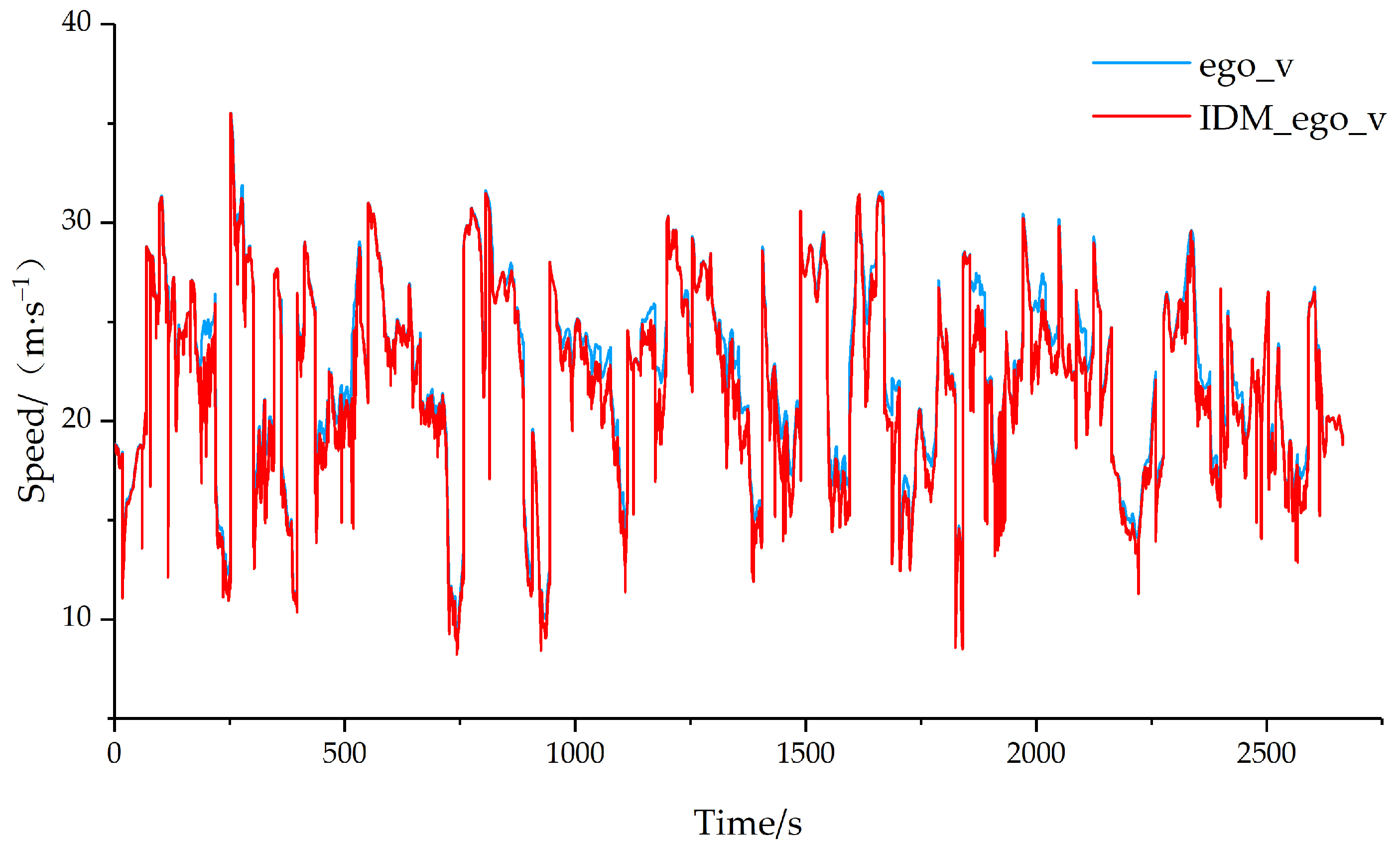
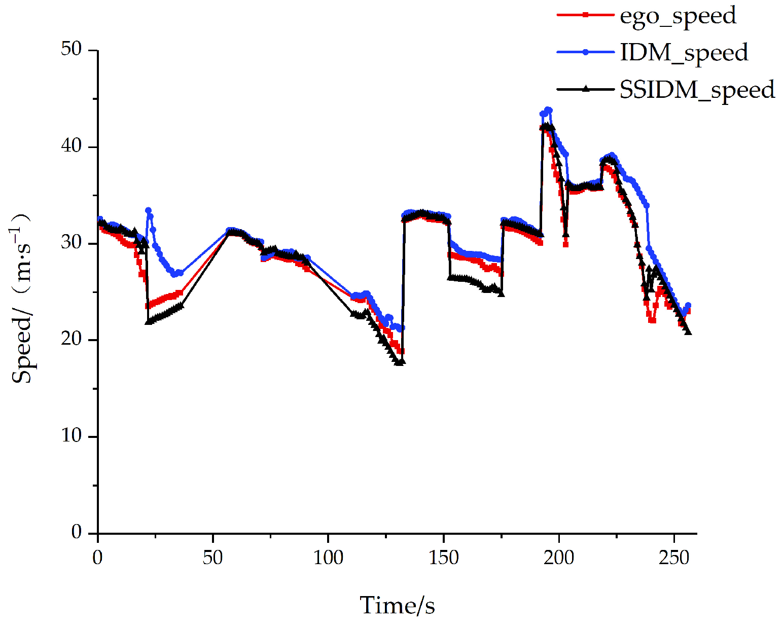
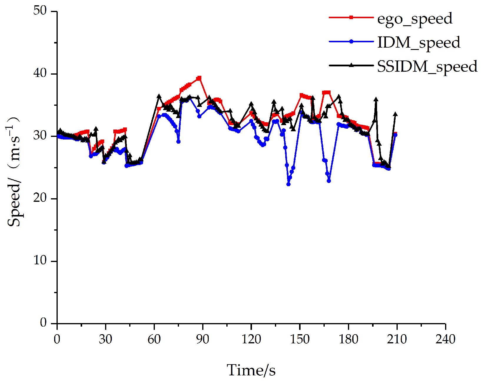
5.2. Comparison of Results

For the second type of scenario, the test set was input into IDM and SSIDM, respectively. The comparison between the prediction results of the two types of models and the actual speed is shown in Figure 12. Due to the influence of drivers’ driving styles, extremely conservative or aggressive driving styles may lead to differences in prediction results, so MSE is used to compare the accuracy of the two models. Using MSE as the error comparison index, the MSE values of the IDM and SSIDM are 3.113 and 2.962.

For the third type of scenario, the test set was input into IDM and SSIDM, respectively, and the comparison between the prediction results and the actual speed is shown in Figure 13. The MSE values of the IDM and SSIDM are 10.647 and 3.383.

For the fourth type of scenario, the test set was input into IDM and SSIDM, respectively, and the speed prediction results of the ego vehicle were compared with the actual speed, as shown in Figure 14. The MSE values of the IDM and SSIDM are 2.582 and 1.238.

The comparison error of IDM and SSIDM on the ego vehicle speed prediction for the second, third and fourth types of scenarios are shown in

Table 5. Error comparison results.

Model	Second Type	Third Type	Fourth Type	Mean Value
IDM	3.113	10.647	2.582	5.169
SSIDM	2.962	3.383	1.238	2.172

.

By adding the constraint components of the front and rear vehicles of the target lane, SSIDM can effectively simulate the acceleration and deceleration of the ego vehicle after reaching the tolerance boundary, according to the analysis of Table 5. Especially in type 3 which is a scenario where there is a rearward vehicle in the target lane. In real driving behavior, in order to obtain sufficient lane-changing space, most drivers will choose to accelerate in the face of the target lane with a rear vehicle. However, for the IDM, its generalized expression is to slow down when approaching the front vehicle and accelerate when moving away from the front vehicle. Therefore, the error value of IDM is the largest for the scenarios of type 3. SSIDM is more accurate compared to the IDM because it takes into account the influence of the rear vehicle in the target lane. The vehicle speed prediction accuracy of SSIDM is greater than that of the traditional single-line IDM, and the mean value of MSE is 57.98% less than that of the IDM.

6. Conclusions

(1) The main goal of this study is to construct a stepless switching model between car-following behavior and lane-changing behavior on basis of the IDM.

(2) This research can provide theoretical support for the construction of the point-to-point driving model and the development of L2+ autonomous driving functions.

(3) The mechanism of switching between the car-following behavior and lane-changing behavior was analyzed. Based on whether there were constrained vehicles in the target lane or not, all segments were divided into four categories. Combined with the first type of scenario, the tolerance boundary was fitted based on the elliptic equation, and the goodness of fitting is 0.572. Based on this boundary, the target lane vehicle constraint components were added to construct SSIDM. The model consistently expresses the coherent driving behavior that can encompass normal following, generate lane-changing intention, and create lane-changing space and speed gains. The two component balance coefficients of SSIDM were identified and calibrated based on the GA method, and the prediction results of IDM and SSIDM were verified by the real vehicle data set.

(4) The prediction results of IDM and SSIDM for the second, third and fourth scenarios were validated through a comparison with the actual collected data. The average MSE for SSIDM is 2.172, which is 57.98% less than IDM. Therefore, the SSIDM considering the tolerance boundary and adding the vehicle constraints of the target lane can simulate the acceleration and deceleration to create lane-changing space and speed gains to equivalent driver behavior. SSIDM can also achieve the car-following behavior to lane-changing behavior stepless switching, with higher accuracy than that of IDM for a single lane.

References

1. Miao, L.; Wang, F. Review on Research and Applications of V2X Key Technologies. Chin. J. Automot. Eng. 2020, 10, 1–12. [Google Scholar]
2. Cao, X. Motion Control and Decision Planning for Car Following and Lane Changing of Autonomous Vehicle. Ph.D. Dissertation/thesis, Jilin University, Changchun, China, 2022. [Google Scholar]
3. Zhu, M.; Wang, X.; Tarko, A.; Fang, S. Modeling Car-following Behavior on Urban Expressways in Shanghai: A Naturalistic Driving Study. Transp. Res. Part C Emerg. Technol. 2018, 93, 425–445. [Google Scholar] [CrossRef]
4. Wang, X.; Sun, P.; Zhang, X.; Zhang, K. Calibrating Car-following Models on Freeway Based on Naturalistic Driving Data. China J. Highw. Transp. 2020, 33, 132–142. [Google Scholar]
5. Treiber, M.; Hennecke, A.; Helbing, D. Congested Traffic States in Empirical Observations and Microscopic Simulations. Phys. Rev. E Stat. Phys. Plasmas Fluids Relat. Interdiscip. Top. 2000, 62, 1805–1824. [Google Scholar] [CrossRef]
6. Péter, T.; Háry, A.; Szauter, F.; Szabó, K.; Vadvári, T.; Lakatos, I. Mathematical Description of the Universal IDM-some Comments and Application. Acta. Polytech. Hung. 2023, 20, 99–115. [Google Scholar] [CrossRef]
7. Qin, P.; Pei, S.; Yang, C.; Meng, Q.; Wan, Q. Influence of Road Geometrics on Car-following of the Intelligent Driver Model. J. Transp. Syst. Eng. Inf. Technol. 2017, 17, 77–84. [Google Scholar]
8. Yi, Z.; Lu, W.; Xu, L.; Qu, X.; Ran, B. Intelligent Back-looking Distance Driver Model and Stability Analysis for Connected and Automated Vehicles. J. Cent. South Univ. (Sci. Technol.) 2020, 27, 3499–3512. [Google Scholar] [CrossRef]
9. Sharath, M.; Velaga, N. Enhanced Intelligent Driver Model for Two-dimensional Motion Planning in Mixed Traffic. Transp. Res. Part C Emerg. Technol. 2020, 120, 102780. [Google Scholar] [CrossRef]
10. Li, Y.; Lu, X.; Ren, C.; Zhao, H. Fusion Modeling Method of Car-Following Characteristics. IEEE Access 2019, 7, 162778–162785. [Google Scholar] [CrossRef]
11. Yang, L.; Zhang, C.; Qiu, X.; Wu, Y.; Li, S.; Wang, H. Car-following Behavior and Model of Chinese Drivers under Snow and Ice Conditions. J. Transp. Syst. Eng. Inf. Technol. 2020, 20, 145–155. [Google Scholar]
12. Jin, P.; Yang, D.; Ran, B. Reducing the Error Accumulation in Car-Following Models Calibrated with Vehicle Trajectory Data. IEEE Trans. Intell. Transp. Syst. 2014, 15, 148–157. [Google Scholar] [CrossRef]
13. Chang, X.; Li, H.; Rong, J.; Qin, L.; Yang, Y. Analysis on Fundamental Diagram Model for Mixed Traffic Flow with Connected Vehicle Platoons. J. Southeast Univ. Nat. Sci. Ed. 2020, 50, 782–788. [Google Scholar]
14. Hu, X.; Zheng, M.; Zhao, J.; Long, B.; Dai, G. Stability Analysis of Mixed Traffic Flow Considering Personal Space under the Connected and Automated Environment. Appl. Sci. 2023, 13, 3231. [Google Scholar] [CrossRef]
15. Péter, T.; Szauter, F.; Rózsás, Z.; Lakatos, I. Integrated Application of Network Traffic and Intelligent Driver Models in the Test Laboratory Analysis of Autonomous Vehicles and Electric Vehicles. Int. J. Heavy Veh. Syst. 2020, 27, 227–245. [Google Scholar] [CrossRef]
16. Bouadi, M.; Jia, B.; Jiang, R.; Li, X.; Gao, Z. Stochastic Factors and String Stability of Traffic Flow: Analytical Investigation and Numerical Study Based on Car-following Models. Transp. Res. B-Methodol. 2022, 165, 1–33. [Google Scholar] [CrossRef]
17. Wang, Z.; Zhou, X.; Wang, J. An Algebraic Evaluation Framework for a Class of Car-Following Models. IEEE Trans. Intell. Transp. Syst. 2022, 23, 1–11. [Google Scholar] [CrossRef]
18. Qu, D.; Wang, S.; Liu, H.; Meng, Y. A Car-following Model Based on Trajectory Data for Connected and Automated Vehicles to Predict Trajectory of Human-driven Vehicles. Sustainability 2022, 14, 7045. [Google Scholar] [CrossRef]
19. Yuan, W.; Fu, R.; Guo, Y.; Peng, J.; Ma, Y. Drivers Lane Changing Intention Identification Based on Visual Characteristics. China J. Highw. Transp. 2013, 26, 132–138. [Google Scholar]
20. Fu, R.; Zhang, H.; Liu, W.; Zhang, H. Review on Driver Intention Recognition. J. Chang’an Univ. Nat. Sci. Ed. 2022, 42, 33–60. [Google Scholar]
21. Zhu, N.; Gao, Z.; Hu, H.; Lu, Y.; Zhao, W. Research on Personalized Lane Change Triggering Based on Traffic Risk Assessment. Automot. Eng. 2021, 43, 1314–1321. [Google Scholar]
22. Chen, H.; Wang, J. A Decision-making Method for Lane Changes of Automated Vehicles on Freeways Based on Drivers Dissatisfaction. China J. Highw. Transp. 2019, 32, 1–9+45. [Google Scholar]
23. Wang, J.; Gao, C.; Zhu, Z.; Yan, X. Multi-lane Changing Model with Coupling Driving Intention and Inclination. Promet 2017, 29, 185–192. [Google Scholar] [CrossRef]
24. Ji, X.; Fei, C.; He, X.; Liu, Y.; Liu, Y. Intention Recognition and Trajectory Prediction for Vehicles Using LSTM Network. China J. Highw. Transp. 2019, 32, 34–42. [Google Scholar]
25. Guo, Y.; Zhang, H.; Wang, C.; Sun, Q.; Li, W. Driver Lane Change Intention Recognition in the Connected Environment. Phys. A 2021, 575, 126057. [Google Scholar] [CrossRef]
26. Zhao, J.; Zhao, Z.; Qu, Y.; Xie, D.; Sun, H. Vehicle Lane Change Intention Recognition Driven by Trajectory Data. J. Transp. Syst. Eng. Inf. Technol. 2022, 22, 63–71. [Google Scholar]
27. Makridis, M.; Leclercq, L.; Ciuffo, B.; Fontaras, G.; Mattas, K. Formalizing the Heterogeneity of the Vehicle-driver System to Reproduce Traffic Oscillations. Transp. Res. C-Emerg. 2020, 120, 102803. [Google Scholar] [CrossRef]
28. Adavikottu, A.; Velaga, N.; Mishra, S. Modelling the Effect of Aggressive Driver Behavior on Longitudinal Performance Measures During Car-following. Transp. Res. F-Traffic 2023, 92, 176–200. [Google Scholar] [CrossRef]
29. Antin, J.; Wotring, B.; Perez, M.; Glaser, D. Investigating Lane Change Behaviors and Difficulties for Senior Drivers Using Naturalistic Driving Data. J. Saf. Res. 2020, 74, 81–87. [Google Scholar] [CrossRef]
30. Li, X.; Oviedo-Trespalacios, O.; Afghari, A.; Kaye, S.; Yan, X. Yield or Not to Yield? An Inquiry into Drivers’ Behaviour When a Fully Automated Vehicle Indicates a Lane-changing Intention. Transp. Res. F-Traffic 2023, 95, 405–417. [Google Scholar] [CrossRef]
Figure 1. Data acquisition system.
Wevj 14 00242 g001
Figure 2. Drivers’ information statistics.
Wevj 14 00242 g002
Figure 3. The schematic indication of car-following constraints.
Wevj 14 00242 g003
Figure 4. Definition of lane-changing starting point: (a) Distance from lane line. (b) Offset speed.
Wevj 14 00242 g004
Figure 5. Mining scenario screenshots.
Wevj 14 00242 g005
Figure 6. IDM identification comparison results.
Wevj 14 00242 g006
Figure 7. Modeling mechanism.
Wevj 14 00242 g007
Figure 8. Kernel density estimation of key parameters: (a) Relative distance. (b) Speed of the ego vehicle. (c) Speed of the front vehicle.
Wevj 14 00242 g008aWevj 14 00242 g008b
Figure 9. Relationship between the ego vehicle speed and the relative distance of the front vehicle.
Wevj 14 00242 g009
Figure 10. The ego vehicle speed-relative distance of the first type of scenario.
Wevj 14 00242 g010
Figure 11. Elliptic equation fitting results.
Wevj 14 00242 g011
Figure 12. Comparison of the models and the actual speed of the second scenario.
Wevj 14 00242 g012
Figure 13. Comparison of the models and the actual speed of the third scenario.
Wevj 14 00242 g013
Figure 14. Comparison of the models and the actual speed of the fourth scenario.
Wevj 14 00242 g014