Abstract
Multiple object tracking (MOT), as a core technology for environment perception in autonomous driving, has attracted attention from researchers. Combing the advantages of batch global optimization, we present a novel online MOT framework for autonomous driving, consisting of feature extraction and data association on a temporal window. In the feature extraction stage, we design a three-channel appearance feature extraction network based on metric learning by using ResNet50 as the backbone network and the triplet loss function and employ a Kalman Filter with a constant acceleration motion model to optimize and predict the object bounding box information, so as to obtain reliable and discriminative object representation features. For data association, to reduce the ID switches, the min-cost flow of global association is introduced within the temporal window composed of consecutive multi-frame images. The trajectories within the temporal window are divided into two categories, active trajectories and inactive trajectories, and the appearance, motion affinities between each category of trajectories, and detections are calculated, respectively. Based on this, a sparse affinity network is constructed, and the data association is achieved using the min-cost flow problem of the network. Qualitative experimental results on KITTI MOT public benchmark dataset and real-world campus scenario sequences validate the effectiveness and robustness of our method. Compared with the homogeneous, vision-based MOT methods, quantitative experimental results demonstrate that our method has competitive advantages in terms of higher order tracking accuracy, association accuracy, and ID switches.
1. Introduction
Multiple object tracking (MOT) can be defined as localizing various objects in a scene after obtaining a sequence of data (i.e., a series of RGB images) over a period of time from sensors, combining these with data association techniques to accomplish the correct matching of the same object between data frames, and forming the tracking trajectory of each object. MOT has enormous potential in both academia and industry and has gained increasing attention in the fields of computer vision and artificial intelligence [1,2,3]. Autonomous driving is the emerging future of the automotive industry, helping to alleviate traffic congestion, reduce traffic accidents, improve driving safety, meet the various needs of different people groups, etc. [4,5,6]. As a core technology for autonomous driving environment perception, MOT is crucial to tasks such as obstacle avoidance, ego-vehicle route planning, intention recognition, and vehicle control of autonomous driving vehicles.
To realize MOT, two main challenges need to be considered: (1) How to measure the similarity between intra-frame objects, and (2) How to recover identity based on the similarity between objects across frames. Problem (1) involves object feature extraction, while Problem (2) pertains to data association. The object appearance features are important clues for measuring the similarity between objects in MOT. Historically, traditional hand-crafted features like RGB color histograms [7] and Local Binary Pattern Histograms (LBPH) [8] have been commonly used for data association. However, these manually designed features have limitations in fully capturing the semantic information of objects and lack robustness in handling significant appearance variations. As a result, their performance tends to be subpar on MOT benchmarks. Nevertheless, with the emergence and advancement of deep neural networks, specifically Convolutional Neural Networks (CNNs), we have witnessed a remarkable shift in feature extraction. The CNN-based feature extractors have gained widespread popularity in MOT research [9,10,11,12]. These feature extractors possess a hierarchical structure, where different convolutional layers characterize the objects from various perspectives. This enables the extracted features to encode more details and semantic information of the objects, thereby distinguishing them from other appearance-similar objects. In addition, due to the high dynamic and complexity of traffic scenes, the main challenges, including object scale changes, light intensity, occlusion, shadows, etc., which are currently faced in MOT for autonomous driving, also increase the difficulty in extracting features with significant discriminability of the object. Therefore, we employ ResNet50 [13] as the backbone network and design an object appearance feature extraction network based on metric learning, which is trained using triplet loss. The network minimizes the distance between the same objects while maximizing the distance between different objects, resulting in discriminative target appearance features. Furthermore, we introduce a Kalman Filter (KF) with constant acceleration (CA) to achieve accurate prediction of object positions by fusing current observations with past state estimates.
Data association is the core of MOT, which aims to correctly match the detections at the current frame with their historical trajectories, and the calculation of feature affinity between objects and trajectories plays an important role in the process. Most existing methods only calculate the feature affinity between the trajectories of the previous frame and the detections of the current frame, ignoring the trajectories that were not matched at the previous frame. This approach is feasible for the continuously detected objects, but for the reappearing objects caused by disappearance or occlusion, they may be assigned to incorrect trajectories, leading to unnecessary ID switches and reducing the tracking performance. To address this issue, we present how to categorize the trajectories within a temporal window composed of consecutive multi-frame images into active trajectories and inactive trajectories and compute the feature affinity between each category of trajectories and detections separately. Active trajectories and inactive trajectories are defined as follows: during the tracking, if no new detections are added to a trajectory in the current frame, its state is set to inactive, otherwise it is set to active. Additionally, we conjoin the concept of the min-cost flow for global association and propose a temporal window data association method. Specifically, when there is a strong (large) affinity between detections and trajectories, our method solves the min-cost flow problem of the network constructed using the affinity between detections and trajectories, enabling optimal matching between detections and trajectories within the temporal window.
To summarize, we present a novel online MOT framework for autonomous driving utilizing min-cost flow on temporal window. The main contributions are summarized as follows:
- By leveraging the feature extraction capabilities of CNN and incorporating metric learning, we design a three-channel neural network with ResNet50 as the backbone network and a triplet loss as learning function. The network aims to extract object appearance features that possess high discriminability. Simultaneously, we employ the KF with CA motion model to optimize and predict the bounding box information of objects. As a result, we obtain robust object representation features.
- The trajectories within the temporal window are divided into active trajectories and inactive trajectories. The affinities between each category of trajectories and detections are computed based on appearance and motion features. By constructing a sparse affinity network and solving the min-cost flow problem, the data association is performed, leading to a reduction in ID switches.
- The extensive experiments have been conducted on the KITTI MOT dataset and our real-world campus scenario. The ablation study confirms the effectiveness of the key modules. The comparison results between our method and the existing homogeneous, vision-based methods using state-of-the-art evaluation measures show that our method exhibits competitive tracking performance.
2. Related Work
Over the past few decades, researchers have proposed a wide range of solutions for MOT. Existing MOT methods can be categorized into two frameworks based on tracking techniques: tracking-by-detection and joint detection and tracking. The main difference lies in whether there is a tracking module integrated with the object detection network.
2.1. Tracking by Detection
The tracking-by-detection methods have become one of the mainstream approaches for MOT [1,7,8,9,10,11,12,14,15,16]. It is a paradigm for multi-stage object tracking. In this tracking paradigm, the video sequence frames are first subjected to object detection using a detector. Then, a tracker is employed to extract features, and a data association method is used to establish correspondences between objects and trajectories. By repeating these steps frame by frame, the final tracking results are obtained. The tracking-by-detection paradigm usually consists of three main modules: object detection, feature extraction, and data association.
Owing to the powerful feature extraction capabilities of CNNs, object detection for autonomous driving has made significant breakthroughs [17,18,19,20,21,22,23]. Ren et al. [17] proposed Faster R-CNN, which used a Region Proposal Network (RPN) instead of Selective Search to generate Region of Interest (RoI) proposals faster. RPN shared the convolutional layers with Fast R-CNN [18], reducing computational complexity and significantly accelerating object detection. G-RCNN [19] was an innovative object detection model that introduced a unique granule concept in CNN. In unsupervised mode, G-RCNN utilized the granule technique combined with spatiotemporal information to extract more accurate RoIs and efficiently capture the details and contextual information of objects, thereby enhancing the performance of object detection. YOLOv4 [20], with CSPDarknet-53 as the backbone network, introduced the “bag of freebies” and “bag of specials” techniques to improve data augmentation and regularization during training, achieving faster inference. YOLOv4 had been considered to strike the best balance between speed and accuracy. YOLOX [21] utilized an anchor-free, decoupled head techniques that allowed the network to process classification and regression using separate networks, reducing the number of parameters and increasing the inference speed. Edge YOLO [22] was a lightweight object detection framework based on YOLOv4, which was designed for 5G edge computing scenarios. It incorporates channel pruning to significantly reduce the network size and improves the feature fusion method to efficiently reduce GPU resource consumption.
Feature extraction is an essential stage in tracking-by-detection MOT methods, and accurate feature extraction is key to high-quality tracking. The object features in MOT mainly focus on appearance features [7,8,9,10,11,12], motion models [1,14], aggregation features [15,16], etc. The appearance features extraction can be divided into hand-crafted features and CNN-based feature extraction. Hand-crafted features include RGB histograms [7], LBPH [8], etc. However, these features cannot capture the semantic information of the objects and have limited discriminative ability. Since CNNs were introduced to computer vision, it has been used by many researchers for extracting object appearance features. Mykheievskyi et al. [9] proposed a simple CNN to learn the local feature descriptors of objects, and Gonzalez et al. [10] adopted a Multiple Granularity Network. Quasi-Dense Similarity Learning [11] generates hundreds of region proposals for contrastive learning of appearance features by densely sampling image pairs and employs most of the information regions on the image to obtain high-quality appearance features. Ref. [12] utilized the self-attention mechanisms to focus on key information about the objects to obtain reliable appearance feature representations. Some researchers used motion models to represent the object. For instance, LGM [14] solved the long-term tracking problem in MOT by effectively utilizing object local and global motion information that was modeled by the box and tracklet embedding modules, without object appearance features. If only appearance features or motion models are used in MOT methods, then the spatiotemporal correlation of objects will be neglected, leading to tracking failures. Therefore, aggregation features have been proposed. STURE [15] achieved learning of spatiotemporal representations between current candidate detections and historical sequences in a mutual embedding space. By designing diverse loss functions, it was capable of extracting more discriminative representations for detections and sequences, thereby enhancing the current detection features and eliminating the differences among them. Yang et al. [16] projected the position and motion features of each object into an adaptive search window, which matched based solely on the similarity of appearance features. This ensured a better balance between appearance and motion features.
In tracking-by-detection methods, data association between trajectories and detections is crucial. It first calculates the affinity between the trajectories and the detections using the extracted features, and then employs different strategies for matching based on the affinity. MOTSFusion [24] was a closed-loop method that adopts a strategy of track first, reconstruct, and then reconstruct and track again. It synthesized information from trajectory extraction and object reconstruction to achieve accurate tracking and recovery of objects by combining 2D trajectory with 3D object modeling and can handle occlusion and missing objects, improving the efficiency and robustness of tracking. TripletTrack [25] exploited a CNN trained with the triplet loss and a Long Short-Term Memory to extract appearance features and motion features from the tracked and detected objects, respectively, determined the similarity of their features and constructed an affinity matrix using a small affinity network, and then adopted the Hungarian algorithm for association. FAMNet [26] employed Siamese networks for single object tracking of each object in adjacent frames and implicitly obtained the appearance and position information of the objects. It achieved continuous multi-frame end-to-end joint data association training by performing local associations. ByteTrack [2] separated the objects into two categories, high-confidence and low-confidence, based on their detection confidence. For the first matching, KF was adopted to generate the trajectory positions at the next frame. Based on either motion affinity or appearance affinity, an association matrix was constructed, and the Hungarian algorithm was then used to match the high-confidence detections with the trajectories. For the second matching, the Intersection over Union distance was used to compute the affinity between the low-confidence detections, the remaining tracked objects and trajectories from the previous step. The Hungarian algorithm was employed again to complete the matching.
2.2. Joint Detection and Tracking
The joint detection and tracking (JDT) methods typically apply the state-of-the-art detector frameworks as the backbone network. The detection branch and feature extraction branch share the underlying features to accomplish the tasks of object detection and feature extraction, enabling data association and achieving simultaneous object detection and tracking. As the object detection and feature extraction tasks are carried out within the same backbone network, the JDT methods are more efficient. YOLOTracker [3] adopted the Hungarian algorithm for data association. It employed the CSPDarknet-53 network as the backbone network and utilized a path aggregation network to fuse low-resolution and high-resolution features. Additionally, the texture features and semantic information were integrated to reduce inconsistencies in object feature extraction and obtain a more comprehensive object representation. Guo et al. [27] employed ResNet101 as the backbone network and introduced temporal-aware object attention and distractor attention, which enhance object focus and suppress interference. This approach enables better focus on the target and suppression of distractions, leading to collaborative joint optimization between position prediction and embedding association tasks. CenterTrack [28] followed the CenterNet framework and took the current frame, the previous frame, and a heatmap generated based on the centers of tracked objects as inputs. In addition to returning the center point, length, and width of the detected bounding box, the regression branch also returned an extra offset, which was used for tracking prediction. Tokmakov et al. [29] proposed an end-to-end trainable method based on [28], named PermaTrack. It used convolutional gated recurrent units to encode the entire frame for feature mapping estimation. PermaTrack incorporated a spatiotemporal, recurrent memory module to utilize past history and infer the position and identity of objects at the current frame. JDT methods require simultaneous execution of detection and feature extraction tasks, but optimizing these tasks separately can lead to conflicts. To solve it, MOTFR [30] introduced a locally shared information decoupling (LSID) module to separate the detection and feature extraction tasks, effectively addressing their optimization conflicts while ensuring necessary information sharing. MOTFR also incorporated a feature purification module that, combined with the LSID module, utilized extracted object features to guide the optimization of the detection task, further improving tracking performance and enhancing the accuracy of object detection. SegDQ [31] was a Transformer-based method that utilized multi-task learning and dynamic feature queries. It employed a semantic segmentation branch to learn and predict foreground masks, aiding in the extraction of foreground features and bounding box regression for MOT tasks. SegDQ introduced a dynamic query method that generated biased object queries using deep features extracted from the backbone network, enabling more robust prediction of newly detected objects. Cai et al. [32] proposed a Transformer-based method called MeMOT. MeMOT leveraged hypothesis generation to generate object proposals at the current frame, providing an initial point for the tracking task. Additionally, it adopted memory encoding to extract core information from the memory of each tracked object, which was used for feature representation and relational modeling. MeMOT addresses both object detection and data association tasks using memory decoding. By utilizing memory and attention mechanisms, MeMOT can establish long-term connections between objects, resulting in more stable and accurate tracking performance.
3. Method
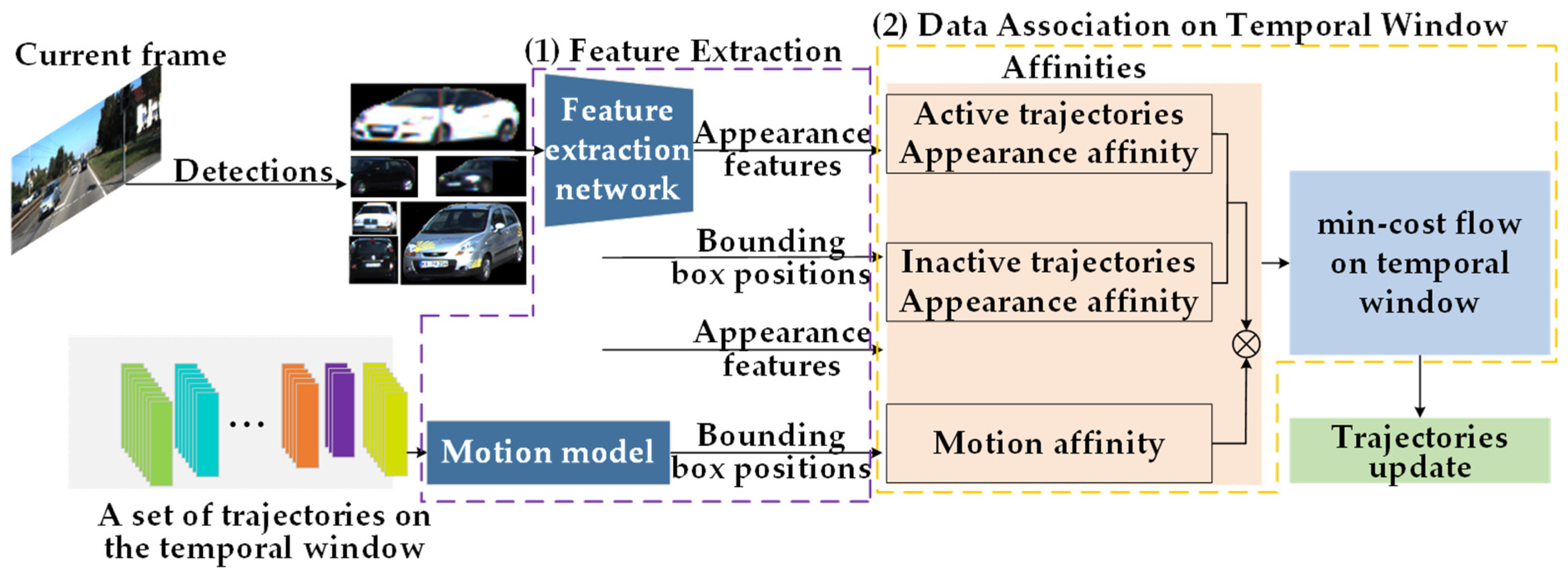
As shown in Figure 1, our proposed online MOT framework follows tracking-by-detection structures. The framework is divided into two parts: feature extraction and data association on the temporal window. In the first stage, our previous work [33] is utilized to accurately segment the objects in the detected bounding boxes by YOLOX [21]. Then, we design an object appearance feature extraction network based on metric learning to obtain discriminative appearance features and apply a motion model to estimate the position information of each trajectory in the trajectories set at the current frame. In the second stage, within a temporal window composed of consecutive multi-frame images and the affinity between inactive trajectories, active trajectories, and detections is computed based on their appearance features and motion affinity. An affinity network is constructed, and the min-cost flow problem of this network is solved to complete the matching between the current frame’s detections and trajectories.
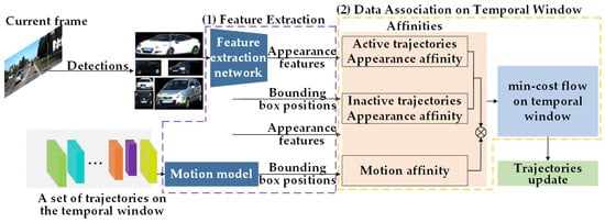
Figure 1.
The overall framework of our method. (1) Feature extraction (in the purple dashed box). (2) Data association on temporal window (in the golden dashed box).
3.1. Feature Extraction
The affinity between detected objects and trajectories is the core of data association in MOT. In this paper, both appearance features and motion features of the objects are adopted during the data association. Specifically, the object appearance features are extracted using a metric learning-based CNN, while the motion features are obtained by predicting the position of the object bounding boxes applying KF.
3.1.1. Feature Extraction
ResNet [13] is a deep neural network under the concept of residual learning. By adding skip connections between convolutional layers, ResNet allows information to propagate across multiple hidden layers, effectively alleviating the problems of gradient vanishing and network degradation that commonly occur in traditional deep neural networks. This enables ResNet to have tens or even hundreds of layers. ResNet50 is one of the variations of ResNet, which has been widely adopted as a backbone or base network in various engineering fields, such as object detection, image recognition, autonomous driving, etc., demonstrating well the feature extraction ability.
In MOT, regardless of the method used to extract object appearance features, an important constraint is that the extracted features must be discriminative, meaning that the affinity between the same object should be high while the affinity between different objects should be low. Therefore, considering the number of parameters and the performance of the model, we choose ResNet50 as the backbone network. Incorporating the metric learning, we design an object appearance feature extraction network, which is shown in the red dashed box in Figure 2.

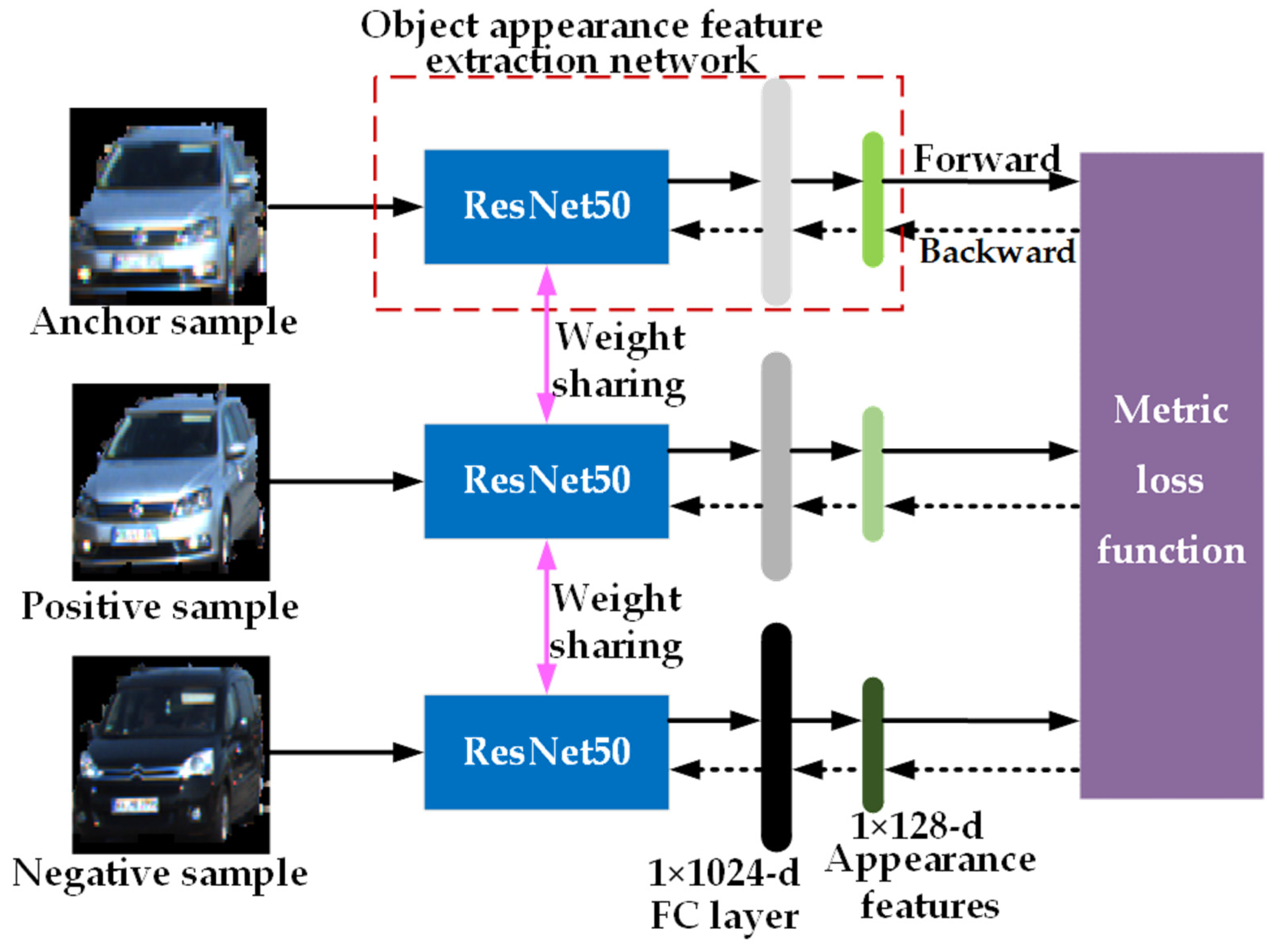
Figure 2.
The flowchart of the object appearance feature extraction network based on metric learning. The network in the red dashed box is our designed network.
From Figure 2, it can be observed that the designed object appearance feature extraction network based on metric learning consists of ResNet50 and two fully connected layers, and outputs a 1 × 128-dimensional vector as the object appearance feature. The specific structure is as follows: the last layer used for classification in ResNet50 is removed, and on top of it, a fully connected layer (FC layer) with 1024 nodes and another fully connected layer (appearance feature layer) with 128 nodes is added. Batch normalization and the ReLU activation function are applied between the FC layer and ResNet50, while no activation function is applied between the FC layer and the appearance feature layer, resulting in a 1 × 128-dimensional object appearance feature vector as the output. During network training, triplets of samples consisting of three images sized 224 × 224 (anchor sample image, positive sample image, and negative sample image) are input into three identical object appearance feature extraction network models with shared weights. Each network model extracts its respective appearance features, and then the metric loss function is computed and backpropagated to optimize and adjust the network weight parameters.
The objective of training the object appearance feature network is to increase the affinity of features belonging to the same object across different frames, while minimizing the affinity between features of different objects, thus the extracted features are discriminative. Therefore, we introduce metric learning and adopt triplet training to map the object appearance features into a metric space, where the affinity between features of the same object is greater than the affinity between features of different objects.
Let the total number of image triplet samples used for training be . The i-th (i = 1, 2,…, ) triplet sample is denoted as , where indicates anchor sample image, denotes positive sample image, and represents the negative sample image. forms a of the anchor-positive pair with , while forms an anchor-negative pair with . The mappings of , , and from the original image space to the learned object appearance feature extraction network feature space are denoted as , , and , respectively. The network is trained using the triplet loss function, , which is commonly used in metric learning techniques:
where, refers to the margin value that allows the network to distinguish between positive sample pairs and negative sample pairs. In other words, the triplet loss learning requires the distance between all negative sample pairs to be greater than the distance between positive sample pairs by a positive minimum margin value . During the training process, the loss continuously decreases, making the anchor samples closer to the positive samples while keeping a larger distance from the negative samples. A smaller means that the anchor samples do not need to be pulled too close to the positive sample set in the feature space, and the anchor samples do not need to be pulled too far from the negative sample set, making it easier to meet the convergence condition. However, since the distance between positive and negative samples is not widened, there is a risk of not being able to effectively distinguish ambiguous data. Conversely, a larger enables better differentiation of similar images with more certainty. However, it brings challenges during the learning process as it requires pulling the anchor points closer to the positive samples and simultaneously increasing the distance from the negative samples, resulting in a larger loss, severe parameter update oscillation, and training difficulties. Therefore, setting a reasonable is crucial for training networks based on triplet loss.
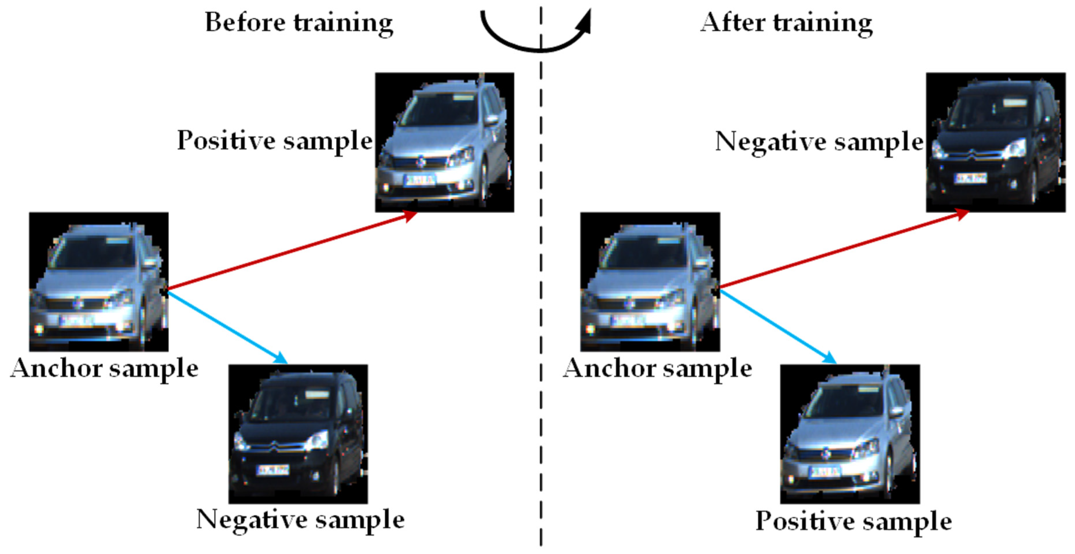
When using the triplet loss function of Equation (1) to train the designed object appearance feature extraction network based on metric learning, the learned feature space not only ensures that the distance of the anchor-positive is smaller than the distance between and , but also incorporates a predefined boundary , which can pull samples of the same object closer and push samples belonging to different objects farther in the learned feature space, as illustrated in Figure 3.

Figure 3.
After training, the distance of the anchor-positive decreases and the distance of the anchor-negative increases.
In addition, when training the network, the gradients of with respect to , , and at the feature extraction layer are given by:
In Equations (3) and (4), is an indicator function: if , the output is 1; otherwise, the output is 0.
3.1.2. Motion Model
In previous MOT methods, the majority use a constant velocity (CV) motion model to predict the future motion states of objects and employ filtering algorithms to smooth the predicted states [34,35]. However, the constant velocity motion model neglects acceleration, which may result in double or more motion errors when the object detector misses detections in consecutive frames. In addition, there are also MOT methods that adopt deep learning (i.e., long short-term memory network) to dynamically model the objects and predict their positions at the current frame. However, compared to previous motion models, this approach requires more time cost. In real-world road scenarios, the objects usually exhibit variable-speed motion, and the motion variation between consecutive frames is relatively small. Therefore, the object motion state can be approximated as uniform variable-speed motion. The Kalman Filter, with its simplicity and low complexity, is widely used for state estimation optimization. Based on the past signal information, it utilizes the principle of statistical computation to optimize the minimum mean square error and predict future state variables. Therefore, to strike a better balance between accuracy and speed, we apply a Kalman Filter with a constant acceleration (CA) motion model to predict and optimize the object position (bounding box) information. Specifically, we model the object motion as a CA motion model and use the measurements obtained from the YOLOX object detector at the current frame. Based on the observation and state transition equations, we iteratively predict and update the object state to obtain the predicted object position at the current frame.
Let be the object state vector, where represents the pixel coordinates of the center point of the object bounding box, is the aspect ratio of the bounding box, denotes the height of the bounding box, , , , and represents the velocities of the corresponding parameters, , , , and represents the accelerations of the corresponding parameters. Assuming the object state vector at the previous frame is , and the YOLOX object detector detects the object state observation value at the frame as . The state transition equation and observation equation for the object are as follows:
where Equation (5) represents the state transition equation, and the state transition matrix indicates the object motion variation. is the process noise, which is a comprehensive abstract description of the uncertainty and random disturbances in the establishment of the motion model, following a normal distribution with zero mean and covariance . is the process noise covariance matrix, caused by uncertain noise. The smaller the , the easier the system converges and the higher confidence in the predicted values of the motion model, but excessively small values may result in divergence. Equation (6) denotes the observation equation, and the observation matrix describes the relationship between the object motion state and the observation. is the measurement noise, similar to the process noise in the state transition equation, obeying a normal distribution with zero mean and covariance . is the measurement noise covariance matrix. In each frame of MOT, it is necessary to predict each object position and update the observation equation and state transition equation corresponding to each object.
The prediction equations are:
where, denotes the posteriori object state estimate of the object at frame , and is the prior (predicted) object state estimate at frame using the CA motion model. Therefore, the predicted state estimate evolves from the optimal estimate (posterior) of the previous state. In this paper, the object motion state is modeled as a CA motion model, and the state transition matrix is as follows:
where denotes the time interval between the capture of two consecutive frames by the camera.
where indicates the 12 × 12-dimensional covariance matrix corresponding to the posteriori object state estimate at frame . represents the 12 × 12-dimensional covariance matrix corresponding to the prior object state prediction at frame , which will be used in the update of the Kalman gain in Equation (10). is the 12 × 12-dimensional process noise covariance matrix.
The updated equations are:
where is the 12 × 12-dimensional identity matrix, is the 12 × 12-dimensional Kalman gain, and represents the 4 × 4-dimensional measurement noise covariance matrix. From observing Equations (10)–(12), it can be seen that the KF estimates the current observation by multiplying the prior state estimate with the observation matrix . The observation residual () is multiplied by the Kalman gain as a correction to the priori state estimate to obtain the object state optimal estimate . Finally, the KF employs Equation (12) to update the posterior estimate covariance , which will be used at the next frame. Equation (12) describes the process of changing the covariance matrix of the state vector, and it is this continuously updated mechanism that allows the Kalman filter to overcome the influence of random noise. In this paper, the observation matrix is:
At this point, a prediction-update iteration process has been completed. In the tracking of each frame, we update the KF for each tracked object, so that we can iteratively predict the each tracked object position (bounding box) information at each frame.
3.2. Data Association by Min-Cost Flow on Temporal Window
We propose an online MOT data association strategy for autonomous driving, which treats trajectories and current detections matching as a min-cost flow problem on a temporal window. First, a sparse affinity network with a finite number of edges is generated using the affinity between trajectories and current detections. Then, the min-cost flow of the network is solved to achieve optimal matching. Finally, the online MOT is realized as the temporal window slides, where the window is composed of consecutive multi-frame images.
3.2.1. Affinity Metrics
Let the set of existing object trajectories in the temporal window be , where represents the active trajectories and represents the inactive trajectories. At frame , the detected object set is denoted as (=1, 2, 3,…, ), where is the total number of detected objects, and for the -th detected object is represented as , where represents the object appearance features and is the bounding box information.
- (1)
- Appearance Affinity Metric
Most tracking-by-detection MOT methods only calculate the appearance affinity between the detections at the current frame and the active trajectories from the previous frame, while ignoring the affinity with the inactive trajectories. This approach is feasible for continuously detected objects, as their appearance changes are relatively small across adjacent frames. However, for objects that reappear due to occlusion or disappearance, this approach can lead to tracking failures and ID switches, as they may not match with their original trajectories. To address the issue, within the temporal window, we calculate the appearance affinity between the detections at current frame and both the active and inactive trajectories separately.
For the active trajectories , the appearance feature vector of the -th trajectory matching detection at frame is . The computation of the appearance affinity between and the detection at frame is as follows:
It can be seen that the smaller the , the more similar the appearance, and vice versa, indicating dissimilarity. It can also be stated that the affinity measurement quantifies dissimilarity, which is determined based on the subsequent requirement of solving the min-cost flow problem.
For the inactive trajectories , calculate the affinity between all appearance features of the -th inactive trajectory and the detection , and take the average as the appearance affinity (dissimilarity) between the inactive trajectory and the detection :
where, indicates the appearance feature vector of the -th detection in the -th inactive trajectory. By performing such calculations, it ensures a more reliable estimation of the affinity between and the inactive trajectory.
- (2)
- Motion affinity metric
We apply the motion model described in Section 3.1.2 to estimate the bounding box positions of all trajectories within the temporal window are estimated at frame , then the motion affinity (dissimilarity) between the trajectory and the detection is measured using the Intersection over Union (IoU) of their respective bounding boxes:
where, represents the prediction of the -th trajectory’s detection at frame , represents the bounding box information of .
3.2.2. Data Association by Min-Cost Flow on Temporal Window
Typically, the min-cost flow is calculated to achieve global optimal matching. In order to apply it in online MOT, we adopt a sliding temporal window approach where global optimal matching is performed within a fixed-length temporal window. Assume that the length of the temporal window is , we obtain the affinities between the detected objects at frames , ,…, , and using Equations (14)–(16). After that, these affinities are utilized to construct an affinity network, which is employed to match the detected objects at frame . The affinity network is a directed graph composed of the following types of nodes:
Source node: Also known as the trajectory start point, it represents a node connected to all object detection nodes with positive costs and is used to initialize a trajectory with a positive cost.
Sink node: Also known as the trajectory end point, it represents a node connected to all object detection nodes with positive costs and is used to terminate a trajectory.
Object detection nodes: In order to satisfy the constraint of non-overlapping trajectories, each detected object in each frame is split into two nodes (pre-node, post-node) with single flow capacity.
Affinity edges: They refer to the edges that connect the object detection nodes, which have the properties of single flow capacity and negative costs.
At frame , the affinity of the detected object with the -th trajectory within the temporal window is calculated as follows:
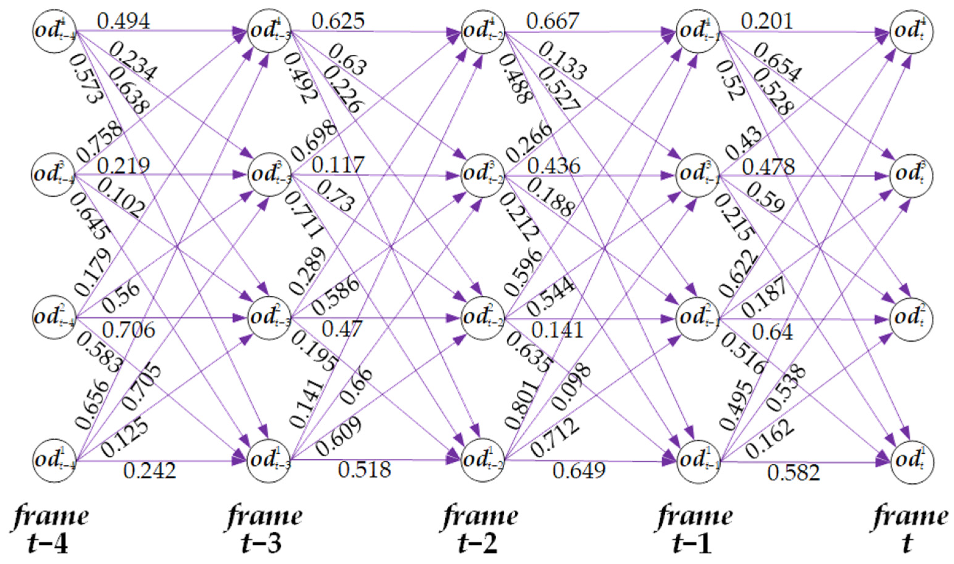
where, if the -th trajectory is an active trajectory, Equation (14) is used to calculate and if it is an inactive trajectory, Equation (15) is employed. Figure 4 illustrates the affinity between trajectories and detections used for constructing the affinity network within a temporal window consisting of 5 consecutive frames, based on Equation (17). In Figure 4, each node (the black circle) represents a detection, and the numerical values on the affinity edges (purple edges) indicate the affinity between two nodes.
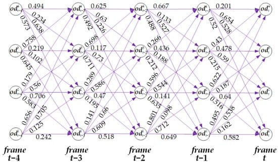
Figure 4.
The illustration of the affinity between trajectories and detections within the temporal window of 5 frames. The nodes are the detections, and the number between two nodes is the affinity.
Let be the affinity edge threshold. In the affinity network, if , a negative-cost affinity edge, , is added between them with a cost of :
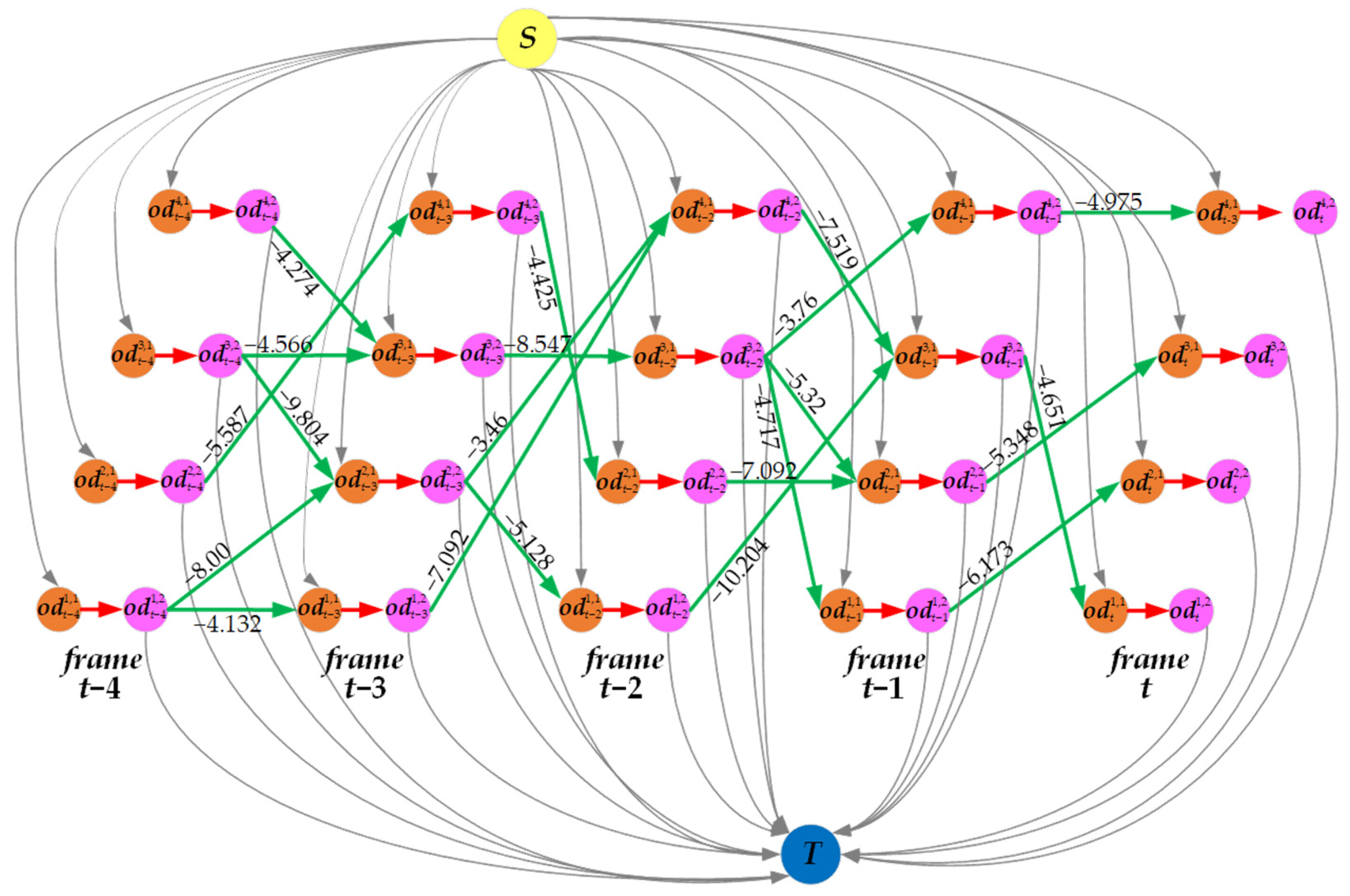
Additionally, we set a maximum number of edges that each object detection node can connect to, ensuring that the out-degree of each object detection node. This limitation reduces the overall number of edges and makes the affinity network sparser. Building upon Figure 4, we construct an affinity network for matching trajectories and detections as depicted in Figure 5. In this example, we set and to 0.3 and 3, respectively.
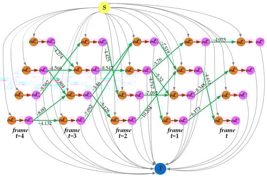
Figure 5.
The sparse affinity network flow graph constructed within the temporal window of 5 frames. S is the source node, T is the sink node, the green edges represent affinity edges with negative costs (the numerical values on the green edges), and orange nodes and pink nodes are the object detection nodes.
In Figure 5, each object detection node is composed of a pre-node (orange node) and a post-node (pink node), connected by a red unidirectional edge, ensuring that any detected objects are passed in a single flow direction (i.e., non-overlapping trajectories). The unidirectional links (green lines) connecting the detected objects between consecutive frames, with negative cost, are referred to as affinity edges. The numerical values on the green edges represent the negative cost values of affinity edges calculated according to Equation (18). The yellow node S is the source node used for initializing trajectories, while the blue node T is the sink node that terminates the trajectories.
Summing up the above, we consider the problem of finding the optimal matching between the objects detected at frame and the trajectories within the temporal window as the task of solving the min-cost flow problem on the constructed sparse affinity network. The min-cost flow is a paradigm widely used to solve data association problems in MOT due to its fast inference and ability to provide globally optimal solutions [36]. Over the years, researchers have developed several effective solutions to solve general min-cost flow problems, including methods like cost scaling, successive shortest path, k-shortest path, etc. However, modifying these methods or directly applying them to MOT may result in computational inefficiency and hinder the application to large-scale problems. To address this, Wang et al. [36] developed a highly efficient and accurate minimum-cost flow solver called minimum-update Successive Shortest Path (muSSP). muSSP updates the shortest path tree only when necessary, i.e., when identifying the shortest S-T path. Experimental results on various MOT public datasets with different object detection results and graph designs have demonstrated that muSSP provides accurate optimal solutions with high computational efficiency. Experimental results on various public MOT datasets with different object detection results and graph designs have demonstrated that muSSP provides accurate optimal solutions with high computational efficiency. Therefore, we adopt muSSP to solve the min-cost flow in the constructed sparse affinity network. After solving it, if an object detected at frame is matched with a trajectory within the temporal window, the object is assigned to the corresponding trajectory and the trajectory is marked as active. If a trajectory within the temporal window does not have any matches with the detected objects, it is marked as inactive. If a detected object is not connected to any trajectory within the temporal window, a new trajectory is initiated with that object as the starting point.
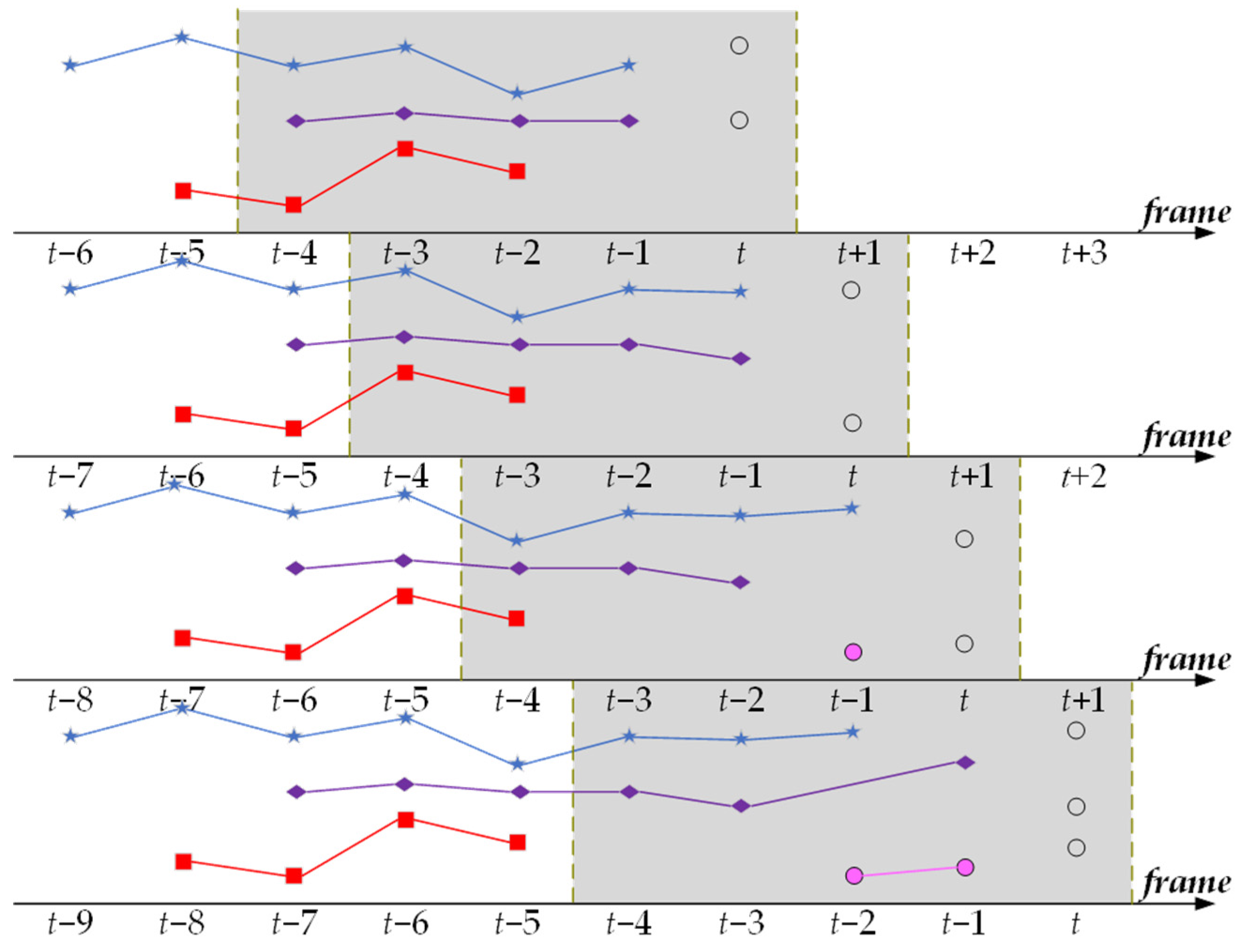
Figure 6 shows an example of trajectory generation at frame . The temporal window consists of a sequence of 5 consecutive frames (masked with gray). The min-cost flow problem in the sparse affinity network is solved within this window. The existing trajectories within the temporal window are displayed as blue, purple, and red lines. The objects detected at frame t are represented by blank circles.
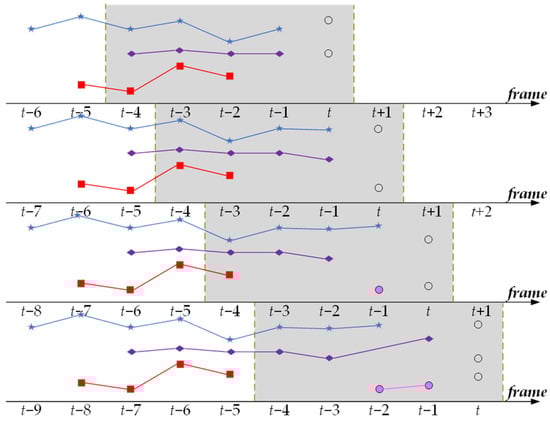
Figure 6.
A diagram illustration for the trajectory generation within a moving temporal window (as masked in gray).
From top to bottom, in Figure 6, we demonstrate how to associate new detections with existing trajectories within the temporal window and how the states of the trajectories are set after the association. In the first row, the two new detections (blank circles) are matched with the purple and blue trajectories, marking them as active trajectories, while the red trajectory is marked as an inactive trajectory. In the second row, one detection is matched to the blue trajectory, while the other detection does not match any purple or red trajectories. The unmatched detection is considered as the starting point of a new trajectory, indicated in pink. At this point, the blue and pink trajectories are active, while the purple and red trajectories are inactive. The two detections in the third row, one is matched to the pink trajectory, and another detection is matched to the inactive purple trajectory. Consequently, the purple and pink trajectories become active, the blue trajectory becomes inactive, and the red trajectory is terminated.
4. Experiments
We conduct experiments on the KITTI MOT dataset [37] and the real-world campus scenario sequences to verify the effectiveness of our method. In this section, we first provide a brief overview of the two MOT datasets. Secondly, we introduce the MOT evaluation metrics. Then, we demonstrate the effectiveness of object appearance features, motion models, and triplet loss function through the ablation study. Additionally, we compare and analyze our method with the existing homogeneous, state-of-the-art, visual-based MOT methods on the KITTI MOT dataset. Finally, we present the intuitive visual tracking results of our method on both two MOT datasets.
4.1. Datasets
4.1.1. KITTI MOT Dataset
The KITTI public benchmark is the first and internationally recognized benchmark dataset for evaluating computer vision methods in autonomous driving [37]. The resolution of the rectified images in the dataset is 1242 × 375 pixels, and each image contains a maximum of 15 cars and 30 pedestrians. The KITTI MOT dataset focuses on tracking classes Car and Pedestrian. It consists of 50 sequences, with 21 sequences for training and 29 sequences for testing. For each sequence, it provides LiDAR point clouds, RGB images, and calibration files. The number of frames used for training and testing is 8008 and 11,095, respectively. For the testing dataset, KITTI does not provide any labels to the users but keeps the labels on the server for MOT evaluation. As for the training dataset, it contains 30,601 objects and 636 tracks. The traffic scenes in the KITTI MOT dataset belong to relatively complex tracking scenarios, involving many challenging factors such as low light conditions, significant lighting variations, frequent occlusions between objects, and the ego vehicle making turns.
4.1.2. Real-World Campus Scenario Sequences
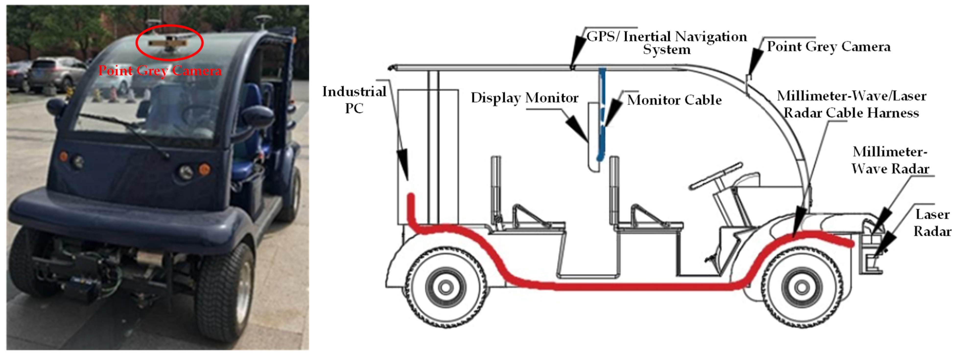
The dataset comprises 10 campus scene sequences, where each sequence consists of images captured during different time periods as the experimental vehicle drives within the campus. The real-world campus scenario images were recorded at a rate of 10 frames per second, capturing varying lighting conditions and different locations within the campus. The resolution of the images is 640 × 480 pixels. The experimental vehicle, as shown in Figure 7, is based on the EG6043K Koala sightseeing vehicle and is equipped with several sensors including a millimeter-wave radar (Delphi ESR), a laser radar (IBEO LUX4), a GPS/inertial navigation system (NAV982), an industrial PC (ARK3500), a display monitor, and a grayscale camera (Point Grey Bumblebee XB3 with a focal length of 3.8 mm and a baseline of 120 mm).
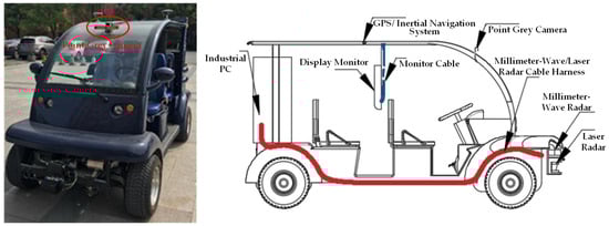
Figure 7.
Illustration of experimental vehicle and sensor installation. (Left): Experimental vehicle. (Right): Diagram of sensor installation.
4.2. MOT Evaluation Metrics
To objectively evaluate the performance of MOT methods, we utilize the following commonly used evaluation metrics in the field of MOT [38,39,40]:
Identity Switches (IDSw): The total number of object identity swaps that occurred throughout the entire tracking process.
Multiple Object Tracking Accuracy (MOTA): This metric is one of the most important evaluation metrics for MOT. It is calculated based on false positives (FP), false negatives (FN), and identity switches (IDSw) as follows:
where represents the number of ground truth annotations at frame . represents the number of objects in the tracking results at frame that do not exist in the ground truth annotations. In other words, these are tracking results that cannot be correctly matched to the ground truth annotations. represents the number of ground truth annotations at frame that are not detected by the tracking results. These are the objects that exist in the ground truth annotations but are not tracked.
Mostly Tracked (MT): represents the ratio of the number of tracks in which the tracking results have a matching rate higher than 80% to the total number of ground truth tracks.
Mostly Lost (ML): represents the ratio of the number of tracks in which the tracking results have a matching rate lower than 20% to the total number of ground truth tracks.
Higher Order Tracking Accuracy (HOTA): A comprehensive metric used for evaluating the performance of MOT methods. It considers both the accuracy of object detection and tracking and weightedly considers the magnitude of tracking errors, providing a more comprehensive reflection of the detection performance (Detection Accuracy, DetA) and tracking performance (Association Accuracy, AssA) of MOT methods. HOTA measures the alignment of matched detection trajectories, averages the entire matched detection, and penalizes unmatched detections. It is recommended to refer to [40] for detailed definitions and analysis of HOTA, DetA, and AssA. Since 25 February 2021, the KITTI MOT dataset ranks the MOT methods based on their HOTA scores in descending order.
For evaluation metrics with quotation marks (), a higher score indicates better performance. On the other hand, for evaluation metrics with a hashtag (), the opposite is true, where a higher score indicates a worse performance.
4.3. Object Appearance Feature Extraction Network Implementation
We implement the proposed object appearance feature extraction network using the TensorFlow deep learning framework, based on the Windows 10 operating system and Python language. Other parameters of the experimental platform used for training the network weights include CPU Intel® Xeon® Silver 4110 @2.1, 16 GB RAM, and Nvidia GeForce GTX1080TI graphics processor (11 GB VRAM). The training dataset consists of samples from the KITTI MOT training sequences and real-world campus scenario sequences. To train the network, we extract the car category objects from the two datasets and perform scale transformation on the object images to obtain a size of 224 × 224 pixels. Additionally, we augment the training images using rotations of 90° and 180°. For constructing triplet images, the anchor samples are primarily taken from unrotated images, negative samples are preferably selected from rotated negative images, and positive samples are randomly chosen from all positive images.
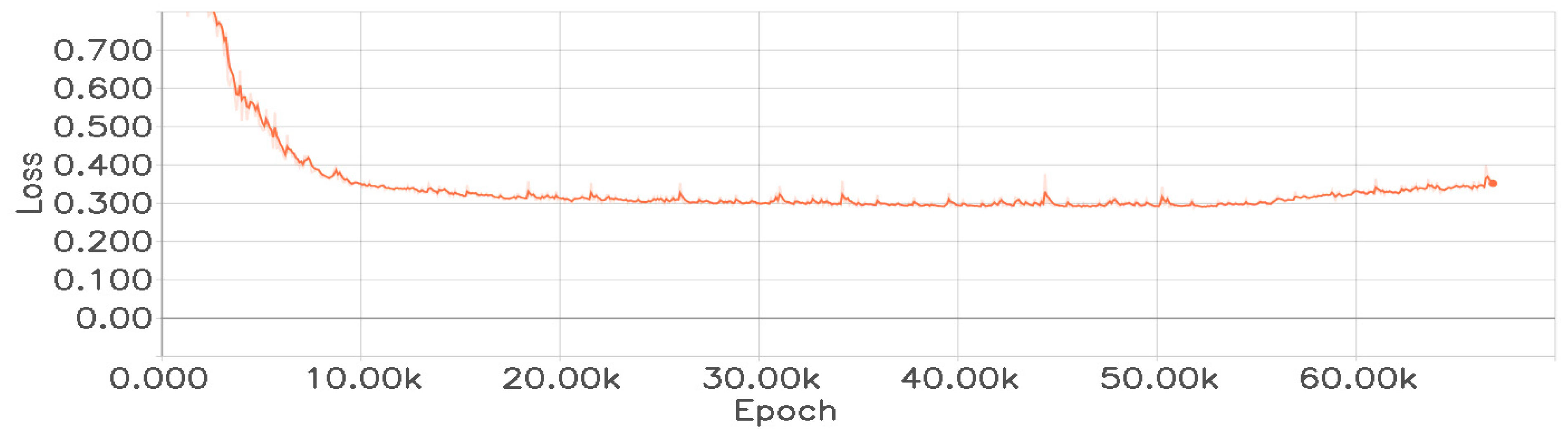
During the training, we do not load any pre-trained weights. All convolutional layers and fully connected layers in the network are initialized with weights following a Gaussian distribution with mean 0 and standard deviation of 0.01. The bias terms are initialized to 0. We employ the Adaptive Moment Estimation optimizer for weight updates. Based on empirical values, the initial value of the learning rate is set to 0.001, the weight decay rate is set to 0.0005, and the momentum is set to 0.900. In the triplet loss function Equation (1), the threshold is set to 0.6. Figure 8 shows our final training loss curve. By observing Figure 8, we can see that the loss value starts to increase at around 52,000th epoch, indicating the occurrence of overfitting. Therefore, when using this network to extract target features, the network weights saved at 50,000th epoch are employed.
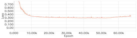
Figure 8.
The loss function curve of the feature extraction network.
4.4. Ablation Study
To better analyze the impact of each component of our method on the overall tracking performance, we conducted an ablation study by individually removing each component from the overall framework. Comparative experiments were then conducted with methods that do not use the respective modules to analyze their effects on MOT. The ablation experiments were conducted on the KITTI MOT training sequences. In the ablation study, the 21 KITTI MOT training sequences were split into training/validation sets. Meanwhile, in order to compare the difference between the triplet loss and the conventional binary loss, we designed and utilized a Siamese CNN without altering the network structure of the object appearance model. We calculated the correlation probability between a pair of detection responses and defined the binary cross-entropy loss to train the object appearance model. The results of the ablation study are shown as Table 1, with the best values highlighted in bold. In Table 1, “seg” represents the extraction of precise object contours prior to extracting object appearance features, while “w/o seg” indicates the absence of object contour extraction, with appearance features directly extracted within the object bounding boxes. “app_T” represents the object appearance features using the triplet loss function, “app_E” represents the object appearance features using the binary cross-entropy loss function, “motion” signifies the object motion information, “ACT” denotes the separation of trajectories within the temporal window into active and inactive trajectories, “w/o ACT” signifies no differentiation of trajectories within the temporal window. The first row is the overall framework of our method, and other rows are the different versions of our method.

Table 1.
Results of ablation study.
Comparing the first row with the second row, we can see that HOTA decreases by 1.88%. This indicates that the approach of first segmenting the objects accurately and then extracting appearance features can significantly improve tracking performance. This is because the segmented bounding boxes only contain the object ontology, without background noise. Thus, the extracted appearance features are less contaminated by noise and can fully represent the object.
Compared to the binary loss (validation loss, corresponding to the third row), using the triplet loss in metric learning techniques can significantly improve the tracking accuracy. HOTA increases from 70.74% to 78.20%, which validates the feasibility of training target feature extraction networks with the triplet loss in MOT.
The fourth and fifth rows validate the impact of different object features on MOT performance. The third row uses only appearance features, while the fourth row uses only the object motion model. Comparing the first row with the third and fourth rows, we can see that although using only appearance features has a certain impact on tracking performance, with a decrease in various evaluation metrics, using only the motion model has the largest impact on tracking performance. The HOTA experiences the largest drop (approximately 5.51%), and other evaluation metrics also show significant decreases. This indicates that various object features have different degrees of impact on MOT performance, and appearance features play an important role in MOT. It also validates the effectiveness of the proposed object appearance extraction network, which can effectively preserve the visual features of the objects.
The sixth row differs from the first row primarily in that trajectory sets within the temporal window are not differentiated as active or inactive during data association. Comparing the two rows, we can observe that when trajectory states within the temporal window are not differentiated, HOTA decreases by approximately 2.25%, while IDSw increases by 10. This suggests that distinguishing trajectory states within the temporal window and matching current frame detections with all trajectories in the temporal window can reduce ID switches caused by occlusion or disappearance and improve MOT performance.
4.5. Comparison with the State-of-the-Art Methods
We upload the testing results of our method on the KITTI MOT testing sequences to the official testing platform of KITTI for easier comparison with other state-of-the-art methods. We compare our method with the existing homogeneous, state-of-the-art, visual-based MOT methods [7,8,10,11,14,24,25,26] in recent years, and the results are shown in Table 2. In Table 2, the best values are highlighted in black bold, while the second-best values are highlighted in blue bold.
Table 2.
Performance comparison results of different tracking methods on the KITTI MOT testing sequences.
As can be seen from Table 2, as the most comprehensive evaluation metric for MOT, our method achieves the highest HOTA, which demonstrates the effectiveness of the proposed MOT method. Further analysis reveals that our method also achieves the best performance in terms of the AssA, with a score of 75.81%, which is the only method that exceeds 75% among all methods. It means that the proposed data association strategy exhibits strong association performance and can maintain the object IDs as much as possible. This is mainly attributed to the following factors: (1) The proposed object appearance extraction network can extract appearance features that adequately represent the objects, and the object motion model based on CA smooths and optimizes the object bounding box information. (2) The data association by min-cost flow on the temporal window considers the classification of inactive and active trajectory states. Unlike other methods that only consider the matching between the current frame detections and the previous frame trajectories, our method matches all trajectories within the temporal window with the current frame detections, allowing reappearing objects to be matched with their historical trajectories to maintain consistent IDs. Additionally, applying the min-cost flow within the sliding temporal window achieves global optimal matching within the temporal window.
Moreover, our method obtains the fewest IDsw (126), which further demonstrates the effectiveness of the proposed MOT method. The data association by min-cost flow on the temporal window reduces ID switches caused by occlusion or disappearance, resulting in stronger robustness for the MOT method. Our method does not achieve the highest DetA score (73.35), which is lower than LGM [14] (74.61) but higher than other comparative methods. This is mainly due to the fact that different methods employ different object detectors, and the performance of various object detectors varies. Despite the relatively lower performance of the object detector utilized in our method, we also acquire better results in terms of HOTA, AssA, and IDsw compared to LGM. It further validates the superiority of our proposed data association strategy by global association on the temporal window. In other words, even in situations where the object detector performance is lower, our method still can effectively address the matching problem between trajectories and detections, leading to improved performance.
From Table 2, among all the MOT methods, our method has a per-frame runtime of 63 ms, which is faster than FAMNET [26], LGM [14], JCSTD [7], SMAT [10], Quasi-Dense [11], TripletTrack [25], and MOTSFusion [24], but slower than MASS [8]. Since the KITTI MOT dataset is captured at a rate of 10 frames per second, selecting an object detection method with a per-frame runtime of no more than 37 ms would ensure real-time performance for the MOT method.
4.6. Visually Intuitive Evaluation
To provide a more intuitive illustration of the performance of our proposed MOT method, in addition to the aforementioned quantitative results, we showcase some qualitative results of our method on the KITTI MOT testing sequences and real-world campus scenario sequences in Figure 9.
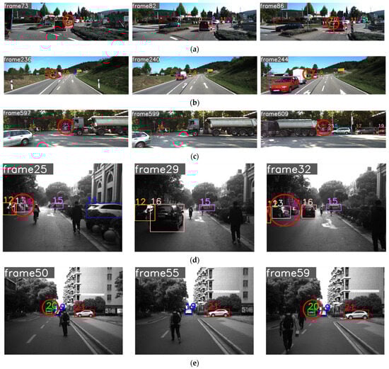
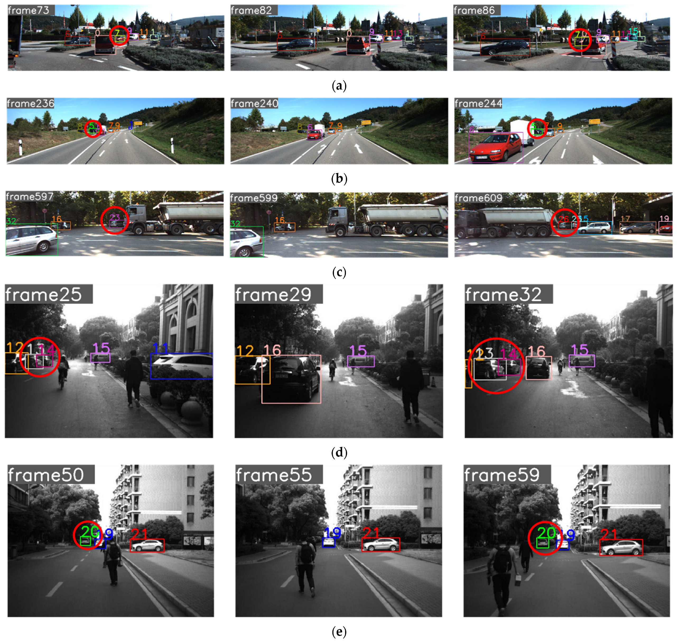
Figure 9.
Tracking results. In each sequence, the tracked cars’ IDs are located at the top of their bounding box, and the objects that will undergo severe or complete occlusion in subsequent frames are marked with red circles. (a) KITTI MOT testing-0008 tracking results. (b) KITTI MOT testing-0009 tracking results. (c) KITTI MOT testing-0015 tracking results. (d) Real-world campus scenarios-0001 tracking results. (e) Real-world campus scenarios-0003 tracking results.
Figure 9a depicts a challenging intersection scene from the KITTI MOT testing sequences, which often involves crossing, overlapping, and occluded objects. It can be observed that at frame 82, Obj. 7 is severely occluded by Obj. 0. However, at frame 86, when Obj. 7 reappears, our proposed method successfully associates it with its historical trajectory. Similarly, in Figure 9b, Obj. 5 is completely occluded, but our method still assigns the correct ID when the object reappears. In Figure 9d, in a real-world campus scenario with poor lighting conditions, Obj. 13, 14 are completely occluded at frame 29. However, our method correctly matches the trajectories with the objects when they reappear. In Figure 9e, Obj. 20 is at a distant distance from the ego-vehicle, but even after being heavily occluded by pedestrians and reappearing, our method maintains its ID. These four examples demonstrate the robustness of our proposed MOT method in various traffic scenarios. Figure 9c shows an example where our method fails. The scenario depicts the ego-vehicle waiting for traffic lights at a traffic intersection. Obj. 23 is under a tree shade and is considerably far from the ego-vehicle. It is completely occluded by a tanker truck at frame 599 and reappears at frame 609. However, our method assigns it the ID 26, resulting in an ID switch. The main reason for this failure is that, during the experiment, the chosen temporal window consists of seven consecutive frames, while Obj. 23 reappears after ten frames. By then, its trajectory is no longer part of the trajectory set within the temporal window, making it impossible to match it with historical trajectory. Since our method uses min-cost flow to match trajectories with detections within the temporal window, the size of the temporal window cannot be arbitrarily increased. A larger temporal window leads to a more complex network, longer computation time to solve the network, and increased runtime of the MOT method. Therefore, the size of the temporal window limits the tracking performance of our MOT method.
In addition, observation of Figure 9 shows that our proposed MOT method accurately associates continuously appearing objects with their corresponding trajectories. It indicates that our method exhibits good association capabilities when dealing with the continuous motion of objects, which helps maintain the uniqueness and continuity of the tracking. This is particularly important in handling objects that temporarily disappear or experience partial occlusion in the sequences. Therefore, our MOT method demonstrates high reliability and accuracy when dealing with continuously appearing objects.
5. Conclusions
In this paper, following the tracking-by-detection pipeline, we present an online multiple object tracking using min-cost flow on temporal window for autonomous driving, which mainly composes of two parts: feature extraction and data association on the temporal window. We apply ResNet50 as the backbone network and design a three-channel network based on metric learning to extract discriminative object appearance features and employ a KF with a CA motion model to optimize the object bounding box information, resulting in reliable and discriminative object representations. In the temporal window composed of consecutive frames, we compute the affinities between the current frame detection and active/inactive trajectories. Based on this, we construct a sparse affinity network and solve the min-cost flow problem on the network to obtain the MOT results. Qualitative and quantitative experiments on the KITTI MOT testing sequences and our real-world campus scenario sequences show that the proposed method outperforms existing visual-based MOT methods of the same type. In the future, we will further optimize the data association strategy to reduce the impact of temporal window length on tracking performance.
Author Contributions
Conceptualization, H.W. and Y.H.; methodology, H.W. and Y.H.; software, H.W.; validation, H.W. and Y.H.; formal analysis, H.W.; investigation, H.W.; writing—original draft preparation, H.W. and Y.H.; writing—review and editing, H.W., Y.H., Q.Z. and Z.G.; project administration, Y.H.; funding acquisition, Y.H. and Q.Z. All authors have read and agreed to the published version of the manuscript.
Funding
This research was funded by the Shanghai Nature Science Foundation of Shanghai Science and Technology Commission, China, grant number 20ZR1437900, and the National Natural Science Foundation of China, grant number 62206114.
Institutional Review Board Statement
Not applicable.
Informed Consent Statement
Not applicable.
Data Availability Statement
All data generated or analyzed during this study are included in this manuscript.
Conflicts of Interest
The authors declare no conflict of interest.
References
- Guo, G.; Zhao, S. 3D multi-object tracking with adaptive cubature kalman filter for autonomous driving. IEEE Trans. Intell. Veh. 2023, 8, 512–519. [Google Scholar] [CrossRef]
- Zhang, Y.; Sun, P.; Jiang, Y.; Yu, D.; Weng, F.; Yuan, Z.; Luo, P.; Liu, W.; Wang, X. Bytetrack: Multi-object tracking by associating every detection box. In Proceedings of the European Conference on Computer Vision (ECCV), Tel Aviv, Israel, 23–27 October 2022. [Google Scholar] [CrossRef]
- Chan, S.; Jia, Y.; Zhou, X.; Bai, C.; Chen, S.; Zhang, X. Online multiple object tracking using joint detection and embedding network. Pattern Recognit. 2022, 130, 108793. [Google Scholar] [CrossRef]
- Abudayyeh, D.; Almomani, M.; Almomani, O.; Alsoud, H.; Alsalman, F. Perceptions of autonomous vehicles: A case study of Jordan. World Electr. Veh. J. 2023, 14, 133. [Google Scholar] [CrossRef]
- Alqarqaz, M.; Bani Younes, M.; Qaddoura, R. An Object Classification Approach for Autonomous Vehicles Using Machine Learning Techniques. World Electr. Veh. J. 2023, 14, 41. [Google Scholar] [CrossRef]
- Liu, Y.; Li, G.; Hao, L.; Yang, Q.; Zhang, D. Research on a Lightweight Panoramic Perception Algorithm for Electric Autonomous Mini-Buses. World Electr. Veh. J. 2023, 14, 179. [Google Scholar] [CrossRef]
- Tian, W.; Lauer, M.; Chen, L. Online multi-object tracking using joint domain information in traffic scenarios. IEEE Trans. Intell. Transp. Syst. 2020, 21, 374–384. [Google Scholar] [CrossRef]
- Karunasekera, H.; Wang, H.; Zhang, H. Multiple object tracking with attention to appearance, structure, motion and size. IEEE Access 2019, 7, 104423–104434. [Google Scholar] [CrossRef]
- Mykheievskyi, D.; Borysenko, D.; Porokhonskyy, V. Learning local feature descriptors for multiple object tracking. In Proceedings of the Asian Conference on Computer Vision (ACCV), Kyoto, Japan, 30 November–4 December 2020. [Google Scholar] [CrossRef]
- Gonzalez, N.F.; Ospina, A.; Calvez, P. SMAT: Smart multiple affinity metrics for multiple object tracking. In Proceedings of the International Conference on Image Analysis and Recognition (ICIAR), Póvoa de Varzim, Portugal, 24–26 June 2020. [Google Scholar] [CrossRef]
- Pang, J.; Qiu, L.; Li, X.; Chen, H.; Li, Q.; Darrell, T.; Yu, F. Quasi-dense similarity learning for multiple object tracking. In Proceedings of the IEEE/CVF Conference on Computer Vision and Pattern Recognition (CVPR), Nashville, TN, USA, 19–25 June 2021. [Google Scholar] [CrossRef]
- Qin, W.; Du, H.; Zhang, X.; Ren, X. End to end multi-object tracking algorithm applied to vehicle tracking. In Proceedings of the Asia Conference on Algorithms, Computing and Machine Learning (CACML), Hangzhou, China, 19–25 November 2022. [Google Scholar] [CrossRef]
- He, K.; Zhang, X.; Ren, S.; Sun, J. Deep residual learning for image recognition. In Proceedings of the IEEE Conference on Computer Vision and Pattern Recognition (CVPR), Las Vegas, NV, USA, 27–30 June 2016. [Google Scholar] [CrossRef]
- Wang, G.; Gu, R.; Liu, Z.; Hu, W.; Song, M.; Hwang, J. Track without appearance: Learn box and tracklet embedding with local and global motion patterns for vehicle tracking. In Proceedings of the IEEE/CVF International Conference on Computer Vision (ICCV), Montreal, QC, Canada, 10–17 October 2021. [Google Scholar] [CrossRef]
- Wang, H.; Li, Z.; Li, Y.; Nai, K.; Wen, M. Sture: Spatial–temporal mutual representation learning for robust data association in online multi-object tracking. Comput. Vis. Image Underst. 2022, 220, 103433. [Google Scholar] [CrossRef]
- Yang, F.; Wang, Z.; Wu, Y.; Sakti, S.; Nakamura, S. Tackling multiple object tracking with complicated motions–Re–designing the integration of motion and appearance. Image Vis. Comput. 2022, 124, 104514. [Google Scholar] [CrossRef]
- Ren, S.; He, K.; Girshick, R.; Sun, J. Faster r-cnn: Towards real-time object detection with region proposal networks. IEEE Trans. Pattern Anal. Mach. Intell. 2017, 39, 1137–1149. [Google Scholar] [CrossRef]
- Girshick, R. Fast r-cnn. In Proceedings of the IEEE International Conference on Computer Vision (ICCV), Santiago, Chile, 7–13 December 2015. [Google Scholar] [CrossRef]
- Pramanik, A.; Pal, S.; Maiti, J.; Mitra, P. Granulated rcnn and multi-class deep sort for multi-object detection and tracking. IEEE Trans. Emerg. Top. Comput. Intell. 2022, 6, 171–181. [Google Scholar] [CrossRef]
- Bochkovskiy, A.; Wang, C.; Liao, H. Yolov4: Optimal speed and accuracy of object detection. arXiv 2020, arXiv:2004.10934. [Google Scholar] [CrossRef]
- Ge, Z.; Liu, S.; Wang, F.; Li, Z.; Sun, J. Yolox: Exceeding yolo series in 2021. arXiv 2021, arXiv:2107.08430. [Google Scholar] [CrossRef]
- Liang, S.; Wu, H.; Zhen, L.; Hua, Q.; Garg, S.; Kaddoum, G.; Hassan, M.M.; Yu, K. Edge yolo: Real-time intelligent object detection system based on edge-cloud cooperation in autonomous vehicles. IEEE Trans. Intell. Transp. Syst. 2022, 23, 25345–25360. [Google Scholar] [CrossRef]
- Xu, H.; Dong, X.; Wu, W.; Yu, B.; Zhu, H. A two-stage pillar feature-encoding network for pillar-based 3D object detection. World Electr. Veh. J. 2023, 14, 146. [Google Scholar] [CrossRef]
- Luiten, J.; Fischer, T.; Leibe, B. Track to reconstruct and reconstruct to track. IEEE Robot. Autom. Lett. 2020, 5, 1803–1810. [Google Scholar] [CrossRef]
- Marinello, N.; Proesmans, M.; Gool, L.V. Triplettrack: 3D object tracking using triplet embeddings and LSTM. In Proceedings of the IEEE/CVF Conference on Computer Vision and Pattern Recognition Workshops (CVPRW), New Orleans, LA, USA, 19–20 June 2022. [Google Scholar] [CrossRef]
- Chu, P.; Ling, H. Famnet: Joint learning of feature, affinity and multi-dimensional assignment for online multiple object tracking. In Proceedings of the IEEE/CVF International Conference on Computer Vision (ICCV), Seoul, Republic of Korea, 27 October–2 November 2019. [Google Scholar] [CrossRef]
- Guo, S.; Wang, J.; Wang, X.; Tao, D. Online multiple object tracking with cross-task synergy. In Proceedings of the IEEE/CVF Conference on Computer Vision and Pattern Recognition (CVPR), Nashville, TN, USA, 20–25 June 2021. [Google Scholar] [CrossRef]
- Zhou, X.; Koltun, V.; Krähenbühl, P. Tracking objects as points. In Proceedings of the European Conference on Computer Vision (ECCV), Virtual Platform, 23–28 August 2020. [Google Scholar] [CrossRef]
- Tokmakov, P.; Li, J.; Burgard, W.; Gaidon, A. Learning to track with object permanence. In Proceedings of the IEEE/CVF International Conference on Computer Vision (ICCV), Montreal, QC, Canada, 10–17 October 2021. [Google Scholar] [CrossRef]
- Kong, J.; Mo, E.; Jiang, M.; Liu, T. Motfr: Multiple object tracking based on feature recoding. IEEE Trans. Circuits. Syst. Video Technol. 2022, 32, 7746–7757. [Google Scholar] [CrossRef]
- Liu, Y.; Bai, T.; Tian, Y.; Wang, Y.; Wang, J.; Wang, X.; Wang, F. Segdq: Segmentation assisted multi-object tracking with dynamic query-based transformers. Neurocomputing 2022, 48, 91–101. [Google Scholar] [CrossRef]
- Cai, J.; Xu, M.; Li, W.; Xiong, Z.; Xia, W.; Tu, Z.; Soatto, S. Memot: Multi-object tracking with memory. In Proceedings of the IEEE/CVF Conference on Computer Vision and Pattern Recognition (CVPR), New Orleans, LA, USA, 18–24 June 2022. [Google Scholar] [CrossRef]
- Wei, H.; Huang, Y.; Hu, F.; Zhao, B.; Guo, Z.; Zhang, R. Motion Estimation Using Region-Level Segmentation and Extended Kalman Filter for Autonomous Driving. Remote Sens. 2021, 13, 1828. [Google Scholar] [CrossRef]
- Wojke, N.; Bewley, A.; Paulus, D. Simple online and realtime tracking with a deep association metric. In Proceedings of the IEEE International Conference on Image Processing (ICIP), Beijing, China, 17–20 September 2017. [Google Scholar] [CrossRef]
- Bewley, A.; Ge, Z.; Ott, L.; Ramos, F.; Upcroft, B. Simple online and realtime tracking. In Proceedings of the IEEE International Conference on Image Processing (ICIP), Phoenix, AZ, USA, 25–28 September 2016. [Google Scholar] [CrossRef]
- Wang, C.; Wang, Y.; Wang, Y.; Wu, C.; Yu, G. muSSP: Efficient min-cost flow algorithm for multi-object tracking. In Proceedings of the Annual Conference on Neural Information Processing Systems (NeurIPS), Vancouver, BC, Canada, 8–14 December 2019. [Google Scholar]
- Geiger, A.; Lenz, P.; Stiller, C. Vision meets robotics: The KITTI dataset. Int. J. Robot. Res. 2013, 32, 1231–1237. [Google Scholar] [CrossRef]
- Bernardin, K.; Stiefelhagen, R. Evaluating multiple object tracking performance: The CLEAR MOT metrics. EURASIP J. Image Video Process. 2008, 2008, 246309. [Google Scholar] [CrossRef]
- Li, Y.; Huang, C.; Nevatia, R. Learning to associate: HybridBoosted multi-target tracker for crowded scene. In Proceedings of the IEEE Conference on Computer Vision and Pattern Recognition (CVPR), Miami, FL, USA, 20–25 June 2009. [Google Scholar] [CrossRef]
- Luiten, J.; Ošep, A.; Dendorfer, P.; Torr, P.; Geiger, A.; Leal-Taixé, L.; Leibe, B. HOTA: A higher order metric for evaluating multi-object tracking. Int. J. Comput. Vis. 2021, 129, 548–578. [Google Scholar] [CrossRef] [PubMed]
Disclaimer/Publisher’s Note: The statements, opinions and data contained in all publications are solely those of the individual author(s) and contributor(s) and not of MDPI and/or the editor(s). MDPI and/or the editor(s) disclaim responsibility for any injury to people or property resulting from any ideas, methods, instructions or products referred to in the content. |
© 2023 by the authors. Licensee MDPI, Basel, Switzerland. This article is an open access article distributed under the terms and conditions of the Creative Commons Attribution (CC BY) license (https://creativecommons.org/licenses/by/4.0/).