Transfer Function-Based Road Classification for Vehicles with Nonlinear Semi-Active Suspension

Abstract

Ride comfort and handling are two important criteria regarding vehicle vibration control. For solving the inconsistency between ride comfort and handling, a semi-active suspension system equipped with a road classification system can be a suitable solution. Because the road condition varies during driving, the control gain of the semi-active suspension system should be adaptively changed according to the road level. In this paper, accelerometer data and a transfer function scheme will be used for road classification, and there is no need to measure the road directly with difficult and often expensive methods. In this approach, a transfer function that makes relevant the Power Spectral Density (PSD) of the road surface and the PSD of car acceleration is used. Road classification is investigated for a vehicle with a nonlinear, semi-active suspension system equipped with Continuous Damping Control (CDC) and nonlinear springs. To show the applicability of the proposed method in scenarios close to real situations, robustness analysis is done by considering vehicle model uncertainties and sensor noise. The simulation results show that the proposed method is robust against typical uncertainties and accelerometer noise and can classify the road level, which is used to tune the parameters of the nonlinear, semi-active suspension system.

1. Introduction

Ride performance is defined regarding vehicular vibrations caused by road roughness, while handling is related to the vehicle’s response to driver input [1]. There are many types of research into solving the inconsistency between ride comfort and handling using a semi-active suspension system equipped with road classification [2]. Because the road condition varies during driving, the control gain of the semi-active suspension system should be adaptively changed according to the road level; thus, a road classification algorithm is needed [2,3,4]. This estimation also is used in active suspension systems [5,6,7]. Many adaptive suspension systems for varying road conditions have been addressed in previous work, such as [8], where the control parameters can be changed adaptively based on the road level.

Semi-active suspension systems offer the best compromise between cost and performance through a variable damping coefficient that can be controlled with the input current [9]. When the road level is estimated, the electronic control unit (ECU) adjusts the input current of the semi-active suspension according to the road level to optimize ride comfort [8].

Some methods, such as direct road measurement and rattle space (the distance between the sprung mass and unsprung mass) measurement, require specific equipment designs that limit their employment. Direct measurement of the road profile using lasers or other devices is a difficult and usually expensive method [10]. Instead, accelerometers are conventionally used by car manufacturers to enhance the suspension system performance [11,12]. In this paper, a road profile classifier is developed utilizing the time history obtained from accelerometers.

Vibration analysis and control of a semi-active suspension system based on a CDC damper was addressed in [13]. A road classification method for a semi-active suspension system was introduced in [14], which was based on Deep Neural Networks (DNNs) and which utilized the skyhook control with a CDC damper. Road profile classification for a vehicle with a semi-active suspension system based on wavelet transform and ANFIS was proposed in [4].

In [15], a flexible neural tree (FNT)-based road profile classification method was proposed for a vehicle with a semi-active suspension system. Wavelet packet transform with a probabilistic neural network (PNN) classifier was utilized in [16], where model predictive control was adopted in a semi-active suspension system.

In [17], an online road profile classification based on unsprung mass acceleration is proposed for a semi-active suspension system, which is based on the root mean square (RMS) of PSD. Road roughness classification through measuring the vehicle acceleration and the artificial neural network has been done in [18].

In [19], vehicle state estimation based on wavelet packet transform with a PNN classifier was proposed. State estimation of the suspension system by using the Adaptive Kalman Filter (AKF) is carried out in [20], in which the wavelet transform with Adaptive Neuro-Fuzzy Inference System (ANFIS) classifier is employed. A road estimation algorithm based on wavelet transform and a double-layer adaptive neural network classifier was used to classify the road level [8]. An Artificial neural network (ANN) was used for classification based on vehicle response [18,21]. Road classification based on wavelet transformation and ANFIS has been addressed by [4].

In [22], a nonlinear road profile classification for a controllable suspension system has been proposed based on feature calculations. A nonlinear controller based on the PNN road classifier was proposed in [23], where the unsprung mass acceleration was used.

A road classification method based on the system transfer function and random forest technique and sprung mass acceleration, unsprung mass acceleration, and rattle space was designed in [24]. In [11], the road class was estimated based on transfer function technique and vehicle acceleration, but a passive and linear suspension system was studied. In [25], the transfer function technique was also used for road classification, but a passive and linear suspension system was studied.

Authors in [2] proposed a road classifier method based on wavelet transform and a PNN, in which a nonlinear suspension system with a CDC damper was used; the control algorithm of the semi-active suspension system was skyhook control. An adaptive neural network control for a semi-active suspension system was proposed in [26], in which a CDC damper was used for the suspension system.

High computational effort and large sets of training data are the well-known disadvantages of the ANN method [25]. Using the wavelet transform and ANN would increase the algorithm complexity; therefore, they are not suitable for real-time and practical applications. The transfer function-based classification method has been addressed in [11,25] and is a simple and fast classification method. In order to overcome the problems of wavelet transform and the ANN method, the present paper uses the transfer function technique. Rattle space measurement is an expensive method with many requirements in [2], while in this paper, only the acceleration of the sprung and unsprung mass is employed.

The International Standards Organization (ISO) offers an approach for classifying road roughness [27]. In this paper, the ISO classification based on the PSD of measured acceleration is used. The approach classifies road roughness as ‘A’ (very good), ‘B’ (good), ‘C’(average), ‘D’(poor) and ‘E’(very poor) [11].

As mentioned above, some works have studied road classification with a passive suspension system; however, the main purpose of road classification is to adjust the controller parameters of a semi-active suspension system. In the present paper, road classification will be carried out for a nonlinear, semi-active suspension system equipped with a CDC damper.

In this paper, the road classifier algorithm is based on the transfer functions that depend on the parameters of the vehicle model. In fact, for practical applications, many transfer functions can be obtained and stored in the computer to be selected based on each vehicle model from the system identification output [28,29,30]. The solution is the combination of model identification and road classification. If system identification techniques are used, the nominal model used to obtain the transfer function and the actual model are almost identical. However, to handle the little differences between the actual model and the nominal model, we intend to analyze the robustness of the classifier against sensor noise and the uncertainties of tire stiffness and vehicle model.

In this work, the following acceleration measurements are used and studied for road level classification: vehicle axle acceleration, and the acceleration of the body center of mass.

The main contributions of this paper are as follows:

The proposed method based on transfer function is fast and simple compared to the methods requiring high computational effort, such as wavelet packet decomposition and neural networks. In addition, this paper proposes an intuitive method that classifies the road level for a semi-active suspension system with a CDC damper. Because the proposed method is simple, it is suitable for practical application. The main purpose of this paper is the combination of a nonlinear, semi-active suspension system and road classification based on the transfer function technique, which has not been addressed in previous works.

The rest of this paper is organized as follows: in Section 2.1, the half-car model is considered as the research object, in which the suspension system is equipped with a nonlinear CDC damper and nonlinear spring; in Section 2.2, road profile generation according to ISO 8608 [27] is presented; in Section 2.3, the algorithm for calculating the PSD of the road is given; in Section 2.4, the transfer function of the half-car model and the road classification algorithm are presented; in Section 2.5, the hybrid controller is designed and analyzed for the various road levels. Then, in Section 3, simulation results and robustness analysis are given. Finally, Section 4 is dedicated to the conclusion.

2. Materials and Methods

2.1. Vehicle Modeling

2.1.1. Governing Equations of the Half-Car Model

In Figure 1, a four-degree-of-freedom (DOF) vehicle model, which is known as the half-car (HC) model, is employed to study the vehicle’s behavior in vertical and longitudinal directions. The HC model has been employed in many works, such as [11,25]. The nonlinear suspension system is equipped with a nonlinear CDC damper and nonlinear springs.

Although a three-dimensional, magic formula of tires model (e.g., as discussed in [31]) should be considered to obtain an accurate model for the vehicle, according to many previous works (e.g., as addressed in [4,6,11,14,15,16] theoretically and in [2,5,7,8] experimentally), in this research, the linear tire model is considered.

The dynamic equations of the HC model are given by Equation (1)

$$\begin{array}{c}{I}_3\ddot{\theta }=L_2{\displaystyle \left[F_{s2}+F_{d2}\right]}-L_1\left[F_{s1}+F_{d1}\right],\\ m_3{\ddot{y}}_3=-\left[F_{s1}+F_{d1}+F_{s2}+F_{d2}\right],\\ m_1{\ddot{y}}_1=\left[F_{s1}+F_{d1}\right]+(m_1+m_{3,1})g-K_t(y_1-q_1(t)),\\ m_2{\ddot{y}}_2=\left[F_{s2}+F_{d2}\right]+(m_2+m_{3,2})g-K_t(y_2-q_2(t)),\\ \begin{array}{ccc}\hfill m_{3,1}& =& m_3\frac{L_2}{L_1+L_2},\hfill \\ m_{3,2}& =& m_3\frac{L_1}{L_1+L_2},\\ y_{3,1}& =& y_3+L_1\theta ,\\ y_{3,2}& =& y_3-L_2\theta ,\\ {\dot{y}}_{3,1}& =& {\dot{y}}_3+L_1\dot{\theta },\\ {\dot{y}}_{3,2}& =& {\dot{y}}_3-L_2\dot{\theta },\end{array}\end{array}$$

(1)

where θ and $y_3$ are the rotation of the sprung body and displacement of the point P₁. The body mass and moment of inertia are $m_3$ and $I_3$, respectively. $m_1$ and $m_2$ are two unsprung masses of the front and rear axles with displacements $y_1$ and $y_2$, respectively. $K_t$ stands for the tire stiffness as a linear spring. The distances from the center of mass of the vehicle to the front axle and rear axle are $L_1$ and $L_2$, respectively. $q_1\left(t\right)$ and $q_2\left(t\right)$ are the road unevenness at the location of the first and second axle. $F_d$ and $F_s$ represent the corresponding CDC damping force and nonlinear spring force, which will be formulated in the next sections. The HC model is stimulated by road excitation.

Regarding the fact that the vehicle body parameters, the tire model, and the nonlinear, semi-active suspension system affect the vehicle’s dynamics and, accordingly, the transfer function, the road classification is affected by them.

According to the three-dimensional magic formula of tires model (e.g., in [31]), the change of vehicle mass and moment of inertia, considering the tire properties and mass properties as constants, will be the sources of uncertainties and affect the performance of the classifier.

In fact, for practical applications, many pre-stored transfer functions can be selected adaptively from the system identification output (e.g., in [28,29,30]). A combination of model estimation and road classification can be a suitable solution to manage uncertain parameters and unmodeled dynamics.

If system identification techniques are used, the actual model and the model used to obtain the transfer function are almost identical. However, to handle the small differences between the real model and the nominal model, the robustness of the classifier against model uncertainties and accelerometer noise will be investigated in this paper.

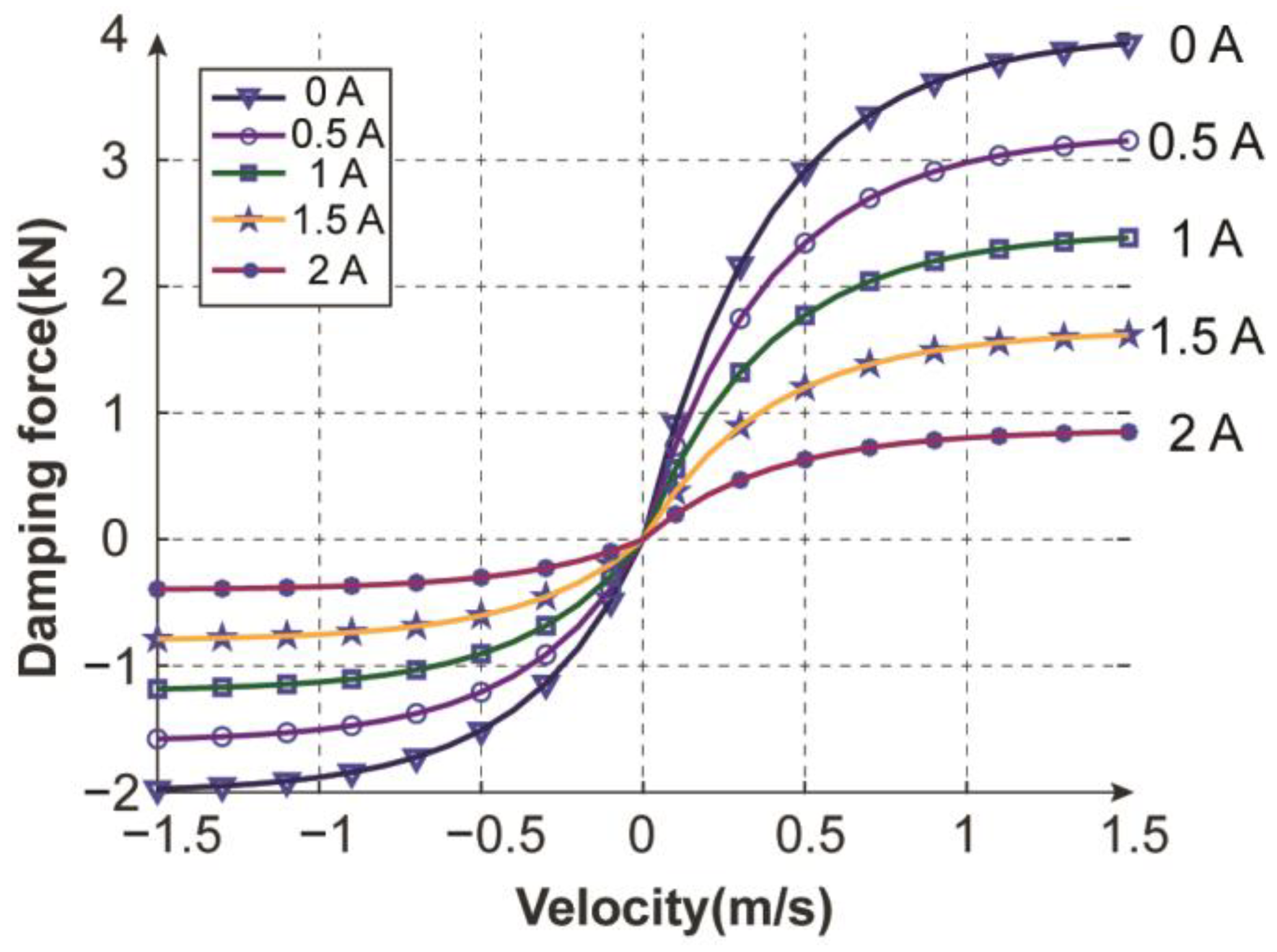
2.1.2. Nonlinear Damping Characteristic Curve

The CDC damper force–velocity characteristic curve is shown in Figure 2 for different input currents. By increasing the input current, the output damping force will decrease.

According to the force–velocity characteristic and by polynomial fitting, the nonlinear model of the CDC damper was derived in [8]. The mathematical model of damping force, which is controlled by input current, is expressed as follows:

$$F_{di}=\left\{\begin{array}{ll}\left(a_0^{+}+a_1^{+}i\right)\left[1-\exp \left(\frac{-b_0^{+}\left|V_{di}\right|}{V_0^{+}}\right)\right]& V_{di}>0\\ 0& V_{di}=0\\ \left(a_0^{-}+a_1^{-}i\right)\left[1-\exp \left(\frac{-b_0^{-}\left|V_{di}\right|}{V_0^{-}}\right)\right]& V_{di}<0\end{array}\right.,i=1,2$$

(2)

where $b_0$ and $V_0$ are the shape parameters. $V_{di}$ is each damper velocity, that is,

$$V_{di}={\dot{y}}_{3,i}-{\dot{y}}_i,i=1,2$$

(3)

Parameters $a_0^{+}$, $a_1^{+}$, $a_0^{-}$, $a_1^{-}$ are given in

Table 1. Parameters of the half-car model with a nonlinear suspension system.

Symbol	Value	Symbol	Value
$m_3(\mathrm{kg})$	650	$a_0^{+}$	4002.75
$m_1(\mathrm{kg})$	42	$a_1^{+}$	−1567.91
$m_2(\mathrm{kg})$	42	$a_0^{-}$	−2002.45
$L_1(\mathrm{m})$	1.44	$a_1^{-}$	801.58
$L_2(\mathrm{m})$	0.96	$b_0^{+}$	3.41
$I_3(\mathrm{kg}{\mathrm{m}}^2)$	750	$V_0^{+}$	1.31
$K_t(\mathrm{N}{\mathrm{m}}^{-1})$	190,000	$b_0^{-}$	9.48
$K_s(\mathrm{N}{\mathrm{m}}^{-1})$	16,000	$V_0^{-}$	3.38
		$\delta$	0.1

. The parameters for extension of the damper are indicated with ‘+’; for compression, they are indicated with ‘-’.

2.1.3. Nonlinear Spring Model

When the deformation of the spring is large it has a nonlinear behavior [8,32], which is written as follows:

$$F_{si}=K_s(y_{3,i}-y_i)+\delta K_s{(y_{3,i}-y_i)}^3,i=1,2$$

(4)

where $K_s$ is the suspension system spring stiffness and δ represents the nonlinear strength parameter (δ > 0).

The vehicle and suspension system parameters of [8] are used in this study. The parameters of the HC model and nonlinear suspension system are given in Table 1.

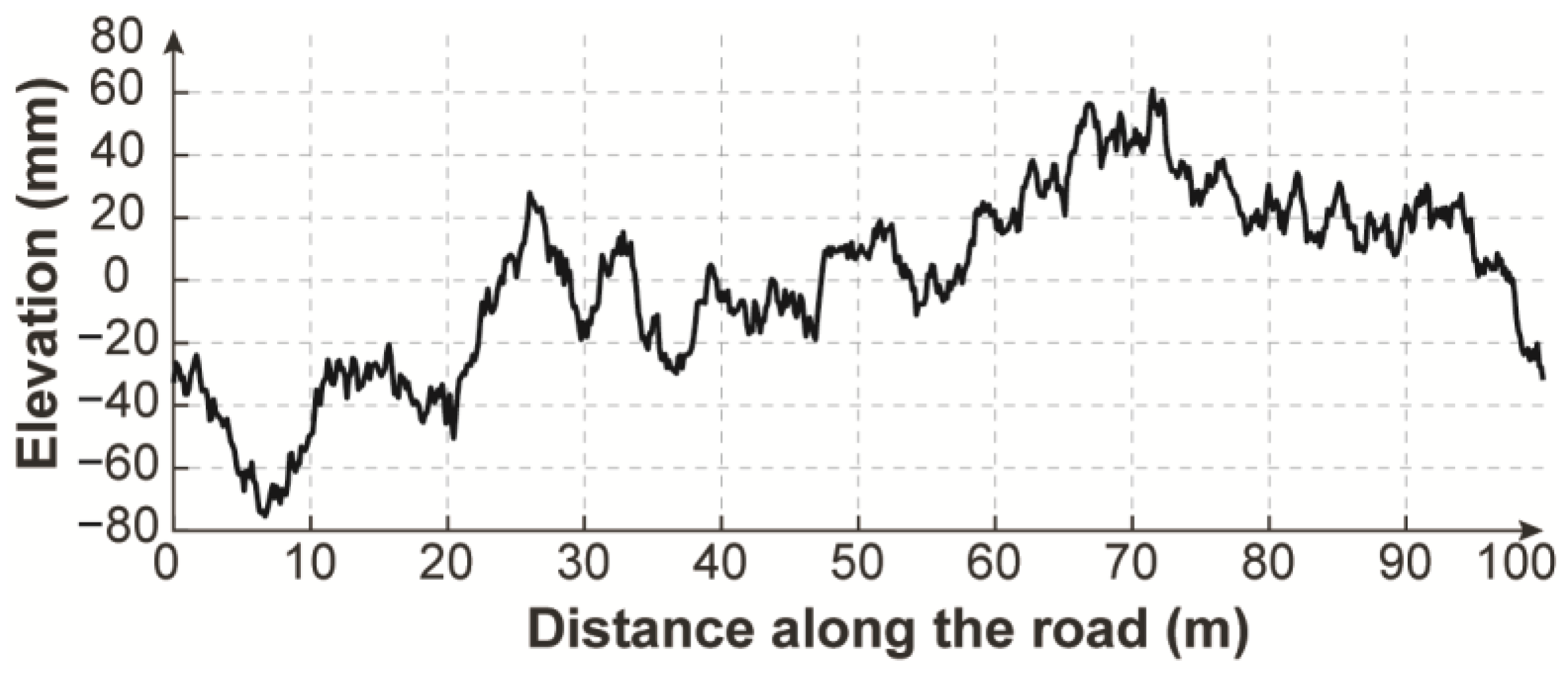
2.2. Road Profile Generation

In order to generate the road irregularity q(t), a suitable mathematical model is needed. The road profile is considered as a Gaussian random process and is characterized by the PSD values. Via the following first-order linear process [33], road irregularity can be generated in the time domain with

$$\dot{q}(t)=-\alpha vq(t)+w(t),$$

(5)

where α stands for the road characteristic parameter in m⁻¹, v is the vehicle velocity in km/h, and w(t) is white noise with covariance.

$${\sigma }_w^2=2{\rho }^2\alpha v,$$

(6)

where $\rho$ is road variance in m. The values of $\alpha$ and $\rho$ are given in

Table 2. Values of road model parameters.

Road Level	$\mathit{\alpha } \mathbf{\left(}{\mathbf{m}}^{-1}\mathbf{\right)}$	$\mathit{\rho } \mathbf{\left(}\mathbf{m}\mathbf{\right)}$
A	0.111	0.0377
B	0.111	0.0754
C	0.111	0.151
D	0.111	0.302
E	0.111	0.603
F	0.111	1.206
G	0.111	2.413
H	0.111	4.825

[33].

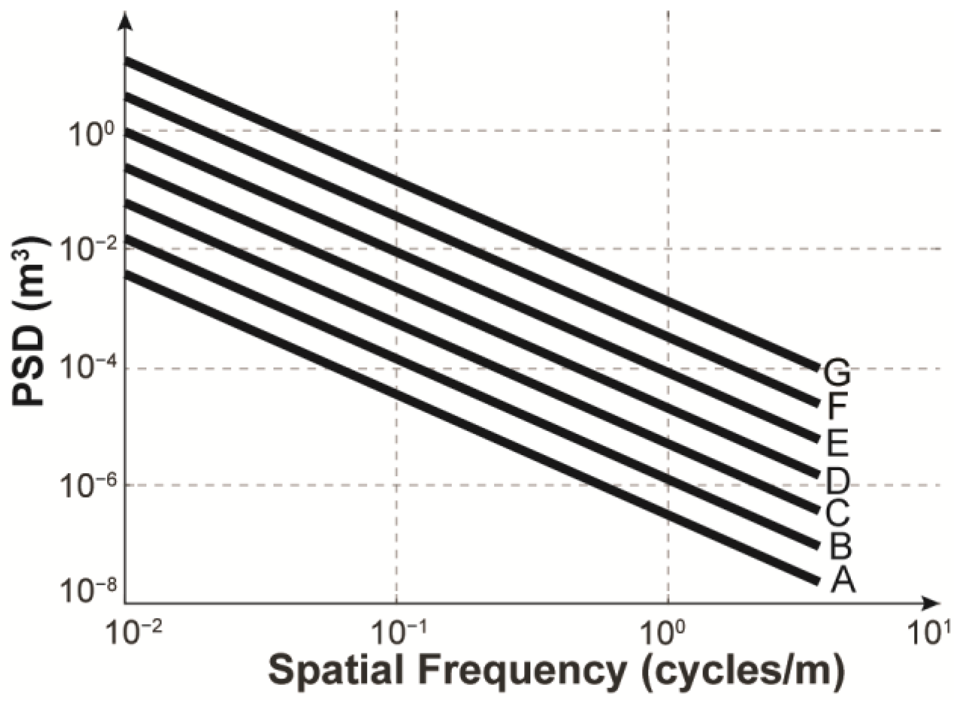
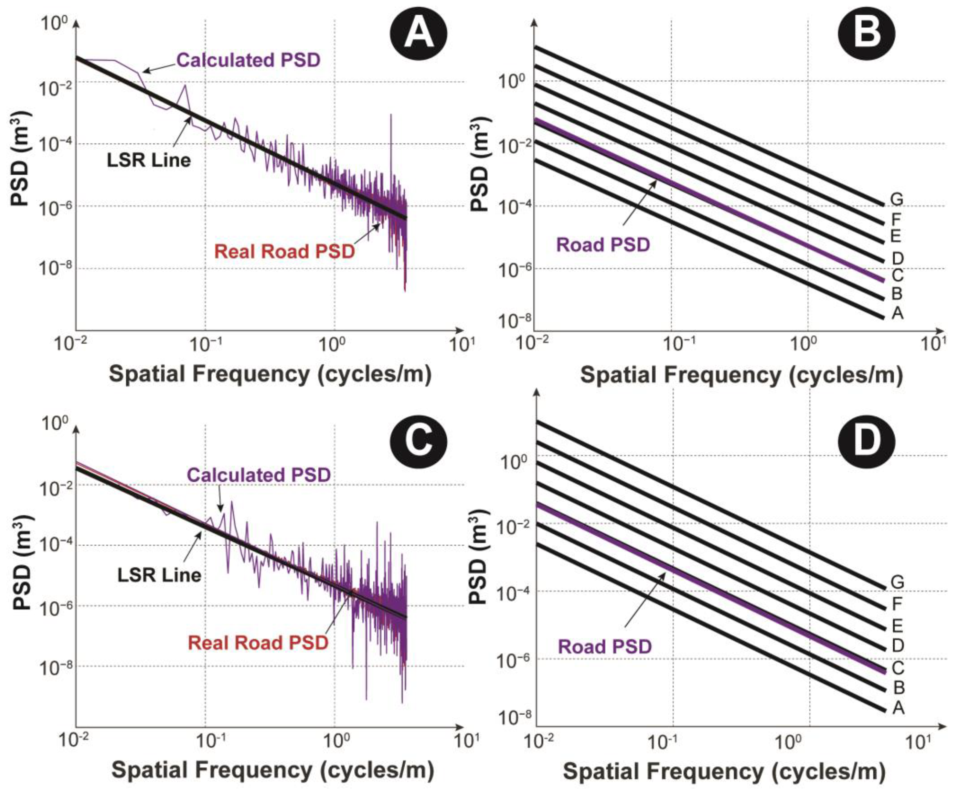
2.3. Calculating the PSD of the Road

PSD is a method for evaluating road roughness. ISO 8608 [27] provides the PSD of a road profile. In Figure 3, the simulated PSD of the original road is illustrated in the special frequency domain. According to ISO 8608, the road is classified into eight levels (A–G).

Because in this paper we need the PSD of each road level, in the following, the procedure of calculating the PSD according to ISO 8608 is presented [34].

The Fourier transform of function q(t), denoted by $Q(f)$ at frequency f, is calculated in the following form:

$$Q(f)={\displaystyle \underset{-\infty }{\overset{\infty }{\int }}q(t)\exp (-2\pi ift)dt}$$

(7)

For digital signal analysis, evaluated at n points as $q(0),\dots ,q(n-1)$, the discrete Fourier transform (DFT) is used:

$$Q(j)={\displaystyle {\sum }_{k=0}^{n-1}q(k)\exp (-2\pi ijk/n)=}{Q}_{\mathrm{Re}}(j)+i{Q}_{\mathrm{Im}}(j),$$

(8)

where $Q_{\mathrm{Re}}(j)$ and $Q_{\mathrm{Im}}(j)$, respectively, stand for the real and imaginary parts. In practice, the fast Fourier transform (FFT) algorithm is implemented, which possesses unique values at half of the frequency domain.

Afterwards, the PSD is given by

$$PSD(j)=\frac{2}{f_{s}n}\left({\left(Q_{\mathrm{Re}}(j)\right)}^2+{\left(Q_{\mathrm{Im}}(j)\right)}^2\right),$$

(9)

in which $j=1,\dots ,n/2+1$ and f_s show the sampling frequency.

It is assumed that a straight line can approximate the PSD [25]. In this paper, the following smoothing algorithm is proposed. By using the smoothing, a uniform distribution of PSD values is obtained over the spatial frequency. Because the calculated PSD is not smooth, the following equations are used to achieve a least square regression line:

$$Y_{ISO,K}=AX+B,$$

(10)

where

$$\begin{array}{c}x={\log }_{10}\left(\mathrm{freq}\right),\\ y={\log }_{10}\left(\mathrm{PSD}\right),\\ c_1={\displaystyle \sum _{i=1}^m{y}_i},c_2={\displaystyle \sum _{i=1}^m{x}_i^2},c_3={\displaystyle \sum _{i=1}^m{x}_i},c_4={\displaystyle \sum _{i=1}^m{x}_i{y}_i},\\ A=\frac{{\mathrm{mc}}_4-{\mathrm{c}}_1{\mathrm{c}}_3}{m{c}_2-c_3^2},\\ B=\frac{{\mathrm{c}}_1{\mathrm{c}}_2-{\mathrm{c}}_3{\mathrm{c}}_4}{m{c}_2-c_3^2},\end{array}$$

(11)

where K varies from 1 to 8 and shows the values of the ISO road (A–H) roughness classification, and

$$X=[\min (x)\min (x)+\sigma \min (x)+2\sigma \dots \max (x)-\sigma \max (x)],\sigma =\frac{\max (x)-\min (x)}{M}$$

(12)

Here the length of M is selected as 100. Finally, the special frequency F and the smoothed PSD for road level K is calculated as

$$\begin{array}{l}F={10}^X\\ PS{D}_{ISO,K}={10}^{Y_{ISO,K}}\end{array}$$

(13)

$PS{D}_{ISO,K}$ will be used in the road classification algorithm.

2.4. Road Classification Algorithm

Because the sprung and unsprung mass of the vehicle is influenced by road irregularities, the measured acceleration of the body and axle can be useful for the estimation of the road PSD. The relationship between the PSD of measured acceleration and the PSD of the road is determined by the transfer function $H(\mathsf{\Omega })$ [35]:

$$H(\mathsf{\Omega })=\frac{PS{D}_{acc}(\mathsf{\Omega })}{PS{D}_{road}(\mathsf{\Omega })}\Rightarrow PS{D}_{road}(\mathsf{\Omega })=\frac{PS{D}_{acc}(\mathsf{\Omega })}{H(\mathsf{\Omega })},$$

(14)

where the PSD of measured acceleration is $PS{D}_{acc}(\mathsf{\Omega })$; $PS{D}_{road}(\mathsf{\Omega })$ will be calculated from the $H(\mathsf{\Omega })$ and the $PS{D}_{acc}(\mathsf{\Omega })$. After calculating $PS{D}_{road}(\mathsf{\Omega })$, the proposed classification algorithm is employed to determine the road’s level. Then the semi-active suspension system will use the estimated road level to adjust the input current of the CDC damper.

$H(\mathsf{\Omega })$ is unknown in practice, but it can be calculated using Equation (14); this transfer function should be calibrated periodically. In this study, according to the ISO model and Equation (5), the road profile will be generated and then the transfer function will be obtained. In Figure 4, the generated random road profile (q(t)) is shown, which is generated using the ISO ‘C’ level and a speed of 50 km/h.

After applying the generated road irregularities to the HC model, the time responses of $y_1,y_2,y_3$ and $\theta$ are calculated and shown in Figure 5.

In this work, four acceleration measurements are used for road level classification: front- and rear-axle acceleration, and the acceleration of two points, P₁ and P₂, on the sprung body, which is shown in Figure 1. The calculated transfer function for front- and rear-axle acceleration as a function of special frequency is given in Figure 6. The calculated transfer function from the acceleration of points P₁ and P₂ are given in Figure 7A,B, respectively. If we have the acceleration of each of the four points via Equation (14), the resulting transfer function will be used for calculating the PSD of the road profile.

The proposed road classification method is presented in the following.

At first, $PS{D}_{road}(\mathsf{\Omega })$ is calculated from the measured acceleration and transfer function (in Figure 6 and Figure 7) by using Equation (14); then a least square regression line is obtained by using the $PS{D}_{road}(\mathsf{\Omega })$ in Equation (11), and we will calculate the $Y_{road}$ of the least square line. Then the road level is calculated from the following optimization problem.

$$\mathrm{Road}\mathrm{Level}=\underset{K}{{\displaystyle \min }}\left({\displaystyle \sum _{i=1}^M{\left(Y_{road}(i)-Y_{ISO,K}(i)\right)}^2}\right)$$

(15)

This method is simple, fast, and easy to implement in real-time.

2.5. Hybrid Control

2.5.1. Skyhook Control

Skyhook control isolates the vehicle body from road disturbances. In this method, between the sprung mass and inertial reference a virtual damper is installed. By considering the passivity constraint (a damper in rebound cannot generate pressure force and a damper in compression cannot generate tension force) of the damper the following control law can be used for the skyhook algorithm [36].

$$F_{sky,i}=\left\{\begin{array}{ll}{c}_{sky}{\dot{y}}_{3,i}& ({\dot{y}}_{3,i}-{\dot{y}}_i){\dot{y}}_{3,i}\ge 0\\ c_{\min }({\dot{y}}_{3,i}-{\dot{y}}_i)& ({\dot{y}}_{3,i}-{\dot{y}}_i){\dot{y}}_{3,i}<0\end{array}\right.,i=1,2$$

(16)

2.5.2. Groundhook Control

Groundhook control is utilized to improve road handling. In this control law, a virtual damper is installed between the unsprung mass and inertial reference. The groundhook control law is:

$$F_{grd,i}=\left\{\begin{array}{ll}{c}_{grd}{\dot{y}}_i& -({\dot{y}}_{3,i}-{\dot{y}}_i){\dot{y}}_i\ge 0\\ c_{\min }({\dot{y}}_{3,i}-{\dot{y}}_i)& -({\dot{y}}_{3,i}-{\dot{y}}_i){\dot{y}}_i<0\end{array}\right.,i=1,2$$

(17)

2.5.3. Hybrid Control

Hybrid control is proposed to combine the advantages of skyhook and groundhook controls. This method is based on the linear combination of the two controllers, shown as follows [36,37,38]:

$$F_{d,i}=\beta F_{sky,i}+(1-\beta )F_{grd,i},i=1,2$$

(18)

where $0\le \beta \le 1$ is the weight for the hybrid control law. The value of $\beta$ can be adjusted according to the road level and the constraints on the suspension system. $\beta =1$ means that comfort is more important and that handling criteria are not considered. $\beta =0$ means that the handling is more important and that comfort criteria are not considered. After calculating the force of each damper, the corresponding current can be calculated from Equation (2).

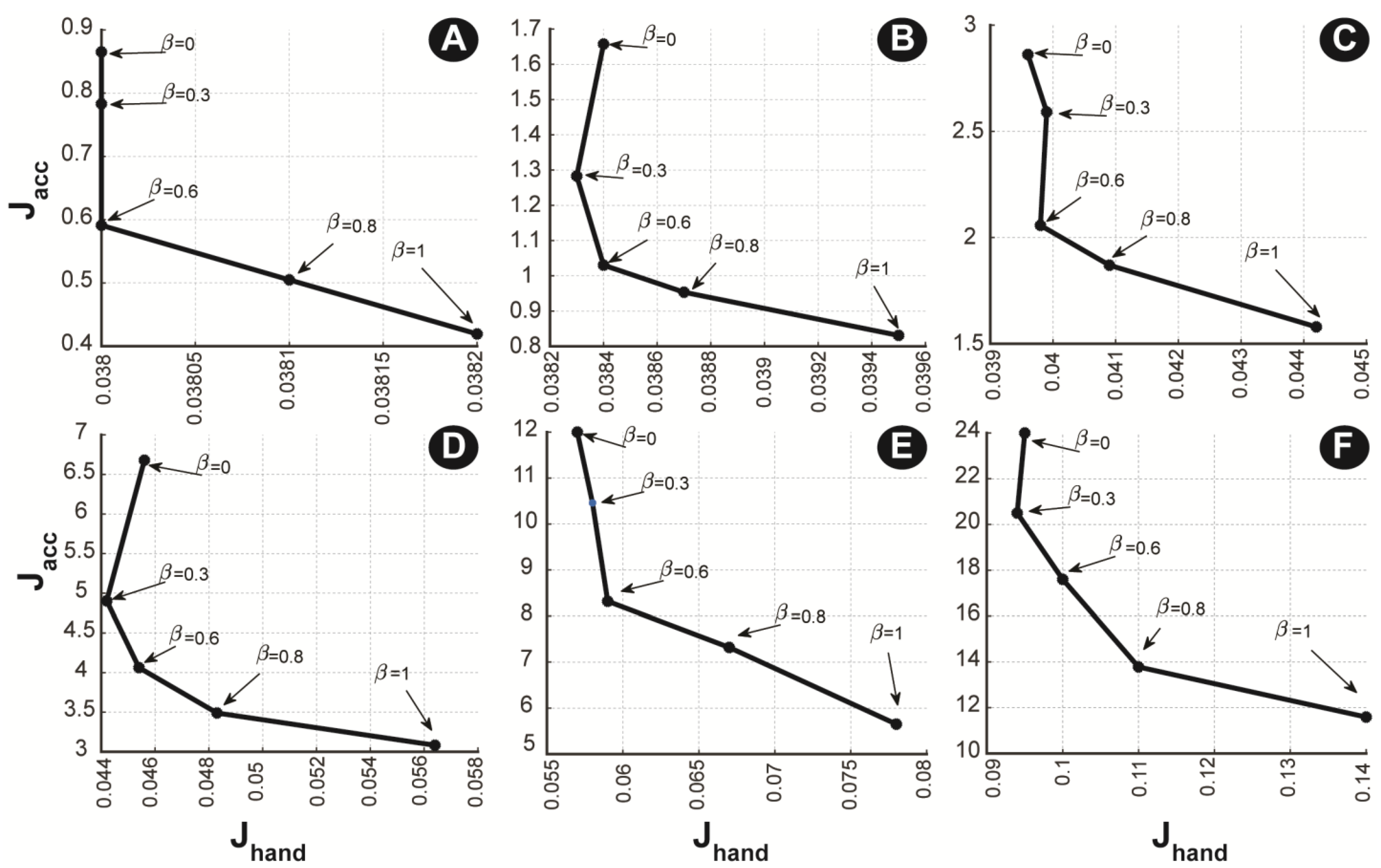
2.5.4. Design of the Parameter $\beta$

One important method for system design is multi-objective optimization [39]. In this subsection, the hybrid controller for $\beta =0,0.3,0.6,0.8,1$ is evaluated, and two values of J_acc (for comfort) and J_hand (for handling) are calculated, where

$$\begin{array}{c}{\mathrm{J}}_{\mathrm{acc}}=\mathrm{rms}\mathrm{(}\ddot{\theta })+\mathrm{rms}({\ddot{y}}_3)\\ {\mathrm{J}}_{\mathrm{hand}}=\mathrm{rms}(y_{3,1}-y_1)+\mathrm{rms}(y_{3,2}-y_2).\end{array}$$

(19)

Here $c_{sky}=c_{grd}=3000\mathrm{N}\mathrm{s}/\mathrm{m}$ and $c_{\min }=300\mathrm{N}\mathrm{s}/\mathrm{m}$ are used. The mentioned results for each road level are given in Figure 8. Note that the aim is to minimize J_acc and J_hand.

In

Table 3. Suspension maximum deflection (in cm) for various road levels and $\beta$.

Road Level	β = 0	β = 0.3	β = 0.6	β = 0.8	β = 1
A	1.5	1.2	1.8	2.2	2.5
B	2	2	1.7	2	3
C	4	3.2	3	3.5	4.5
D	8	7	7	15	8
E	13	14	13	20	20
F	25	25	30	40	40

, the maximum deflection of the suspension system for various road levels and $\beta$ is reported.

Because the road input is stochastic the positions of points on the Pareto front are changed in each simulation, but the deviation is small and negligible.

It is assumed that the road classification logic works accurately; now, we should choose a suitable value of $\beta$ for each road level. At the road level A, for J_hand there is little difference between 0.0382 and 0.038; thus, the point at which $\beta =1$ is selected as the proper point to achieve the best comfort when the vehicle is moving on road level A. Similar to road level A, for road levels B and C, $\beta =1$ is selected as the proper point to achieve the best comfort.

Note that from Table 3 the maximum deflection of the suspension system for each $\beta$ is acceptable for road levels A, B, and C. From Table 3 and Figure 8 (level D), for road level D it is better to choose $\beta =0.6$ to achieve a maximum suspension deflection of 7 cm. Note that if $\beta =0.8$ is selected, a maximum deflection of 15 cm is achieved, which is approximately twice that of 7 cm. For level E, in order to prevent the large value of J_hand, the value of $\beta =0.6$ (with a maximum deflection of 13 cm) is selected as the proper point. Indeed, suspension system designers can select a proper $\beta$ for each road level according to their criteria and the constraints of the suspension system.

3. Results and Discussions

In this section, the performance of the proposed classification algorithm for a vehicle with a nonlinear, semi-active suspension system is investigated. The input current of the CDC damper is the control input of the semi-active suspension system.

A real road is not generated as a special road class, but rather is a combination of road classes; thus, in this paper as in [25], a simulated road is utilized. Therefore, the HC model is excited by the mentioned simulated road unevenness. This paper assumes that the real road level is ‘C’, so the road classification performance will be investigated according to the mentioned road level. In the simulations, the car velocity is V = 50 km/h, and the length of the road is L = 100 m.

In this section, road level classification based on two acceleration measurements is investigated: axle acceleration and the acceleration of points P₁ on the sprung body. The aim is to investigate the effect of the accelerometer location on road classification. In order to better illustrate the performance of the proposed classifier and achieve a robust road classification, the measurement of noise is also considered here.

In the following, by using the vehicle parameters in Table 1, the control law in Equation (11), the damper model in Equation (2), and road level C, the semi-active suspension system is simulated and the root mean squares (RMS) of $\ddot{\theta }$ and ${\ddot{y}}_3$ are reported.

Because road unevenness is a stochastic input, one simulation is not enough; therefore, five simulations have been completed and their results are given in

Table 4. RMS values of $\ddot{\theta }$ and ${\ddot{y}}_3$ for several simulations.

	$\mathit{R}\mathit{M}\mathit{S}(\ddot{\mathit{\theta }})$			$\mathit{R}\mathit{M}\mathit{S}(\ddot{{\mathit{y}}_3})$
No. Simulation	Passive	Hybrid	Passive	Hybrid
1	0.99	0.72	1.23	0.93
2	0.98	0.74	0.95	0.8
3	1	0.69	0.95	0.8
4	1.02	0.75	1.14	0.93
5	1.07	0.79	1.17	0.87

. It is obvious that hybrid control will result in better performance than passive suspension.

The time response of the vehicle body displacement and body angle for semi-active and passive suspension is shown in Figure 9 and Figure 10, respectively. From the time response and the RMS values of $\theta$ and $y_3$ we can conclude that the semi-active suspension has better performance than the passive system.

Robustness Analysis of the Road Classifier

In this section, to manage the differences between the actual model and the nominal model of a vehicle, the robustness of the classifier against the vehicle model and tire uncertainties and accelerometer noise are investigated.

At first, the transfer function $H(\mathsf{\Omega })$ is obtained using the nominal parameter values given in Table 1.

According to the data sheet of accelerometers used in industry, their noise levels are very low. However, to consider the worst-case scenarios, $\sigma =0.05\mathrm{m}/{\mathrm{s}}^2$ and $\sigma =0.2\mathrm{m}/{\mathrm{s}}^2$ are two standard deviations that are considered in this paper. It is worth noting that the mentioned standard deviations are much larger than the values reported for industrial accelerometers.

The noisy acceleration is obtained by adding the noise to the true acceleration. The noise-corrupted acceleration is

$$a_i(t)={\ddot{y}}_i(t)+n(t),i=1:4$$

(20)

where n(t) is the Gaussian white noise with zero mean and a standard deviation of $\sigma$.

Some of the points used to analyze the robustness of the classifier are as follows:

• Road classification is investigated for the following two cases of accelerometer location: 1-on the vehicle axle; 2-on the vehicle body center of mass (P₁)
• Three percentages of 0%, +15% and +30% are considered for the uncertainty levels of vehicle body mass and moment of inertia.
• Three percentages of 0%, ±20% and ±40% are considered for the uncertainty levels of vehicle tire stiffness.
• Two standard deviations, $\sigma =0.05\mathrm{m}/{\mathrm{s}}^2$ and $\sigma =0.2\mathrm{m}/{\mathrm{s}}^2$, are considered for the accelerometer noise levels.
• The classification error index is the cost function value given in Equation (15).
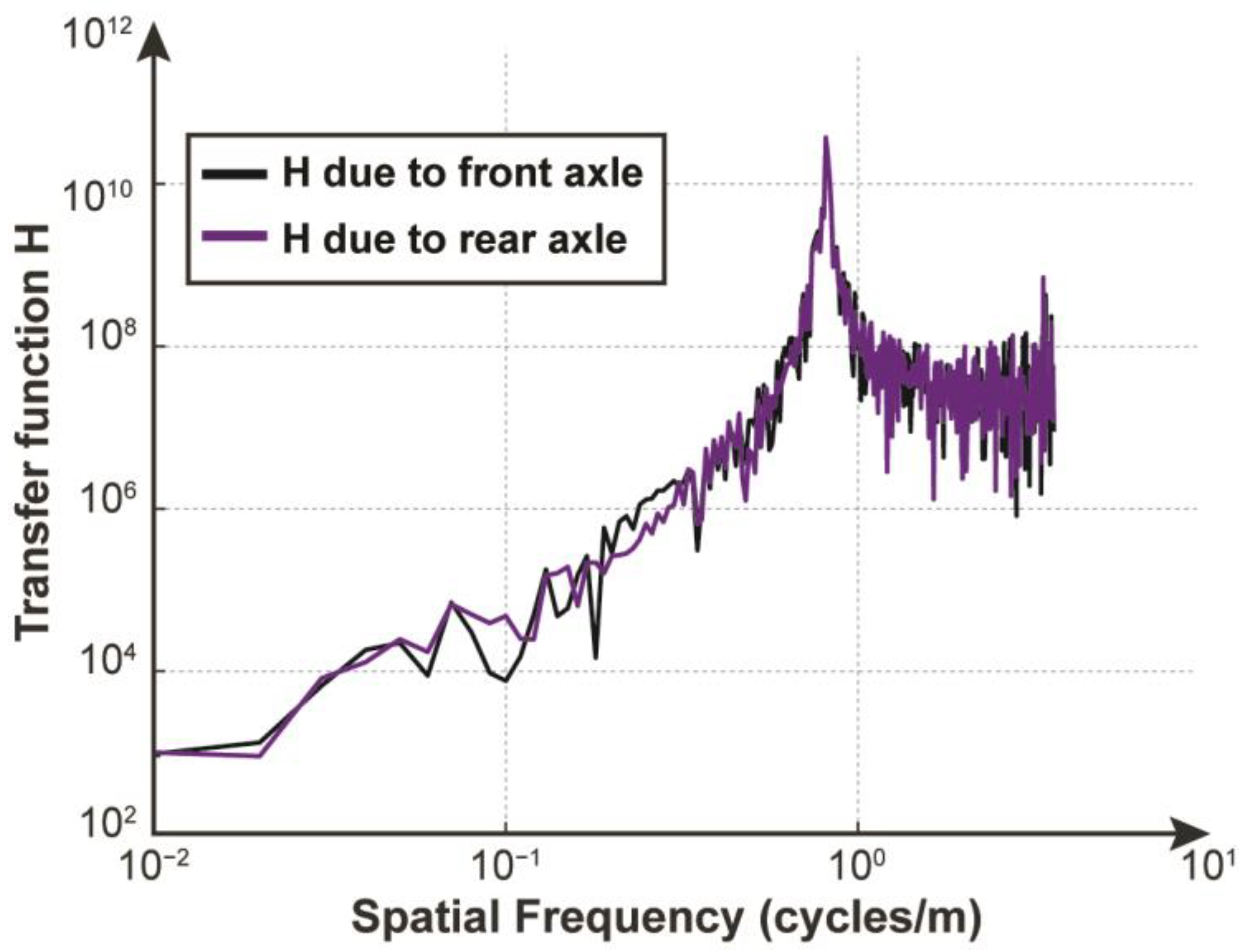
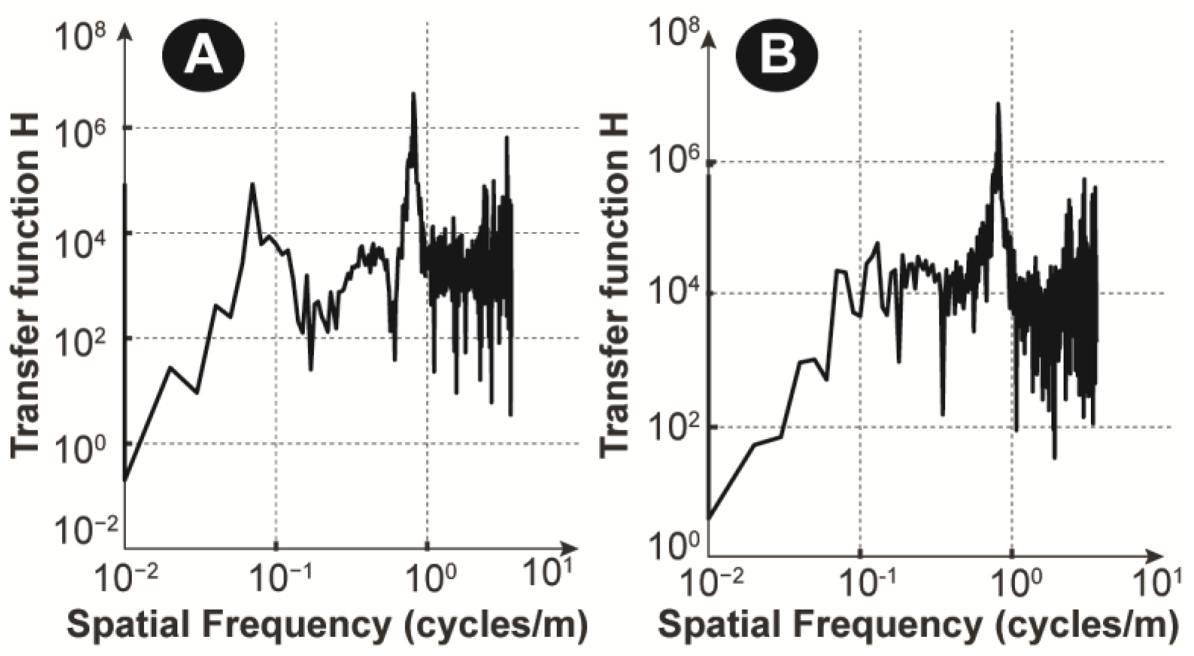
• The road level C and hybrid controller with $\beta =0.8$ are considered for robustness analysis (note that the transfer function does not depend on the road level and only depends on the vehicle model [11]).
• Finally, the road classification algorithm (15) gives the estimated road level automatically.

The robustness analysis of the two possible accelerometer locations is given in

Table 5. Classifier robustness analysis for accelerometer located on the vehicle axle.

Uncertainty of Body Mass Properties	Uncertainty of Tire Stiffness	$\mathit{\sigma }$ (m/s2)	Estimated Road Level	Classifier Error
+30%	±40%	0.05	D (failed)	14.1	1.
		0.2	D (failed)	14.4	2.
	±20%	0.05	C	3.1	3.
		0.2	C	3.71	4.
	0%	0.05	C	0.8	5.
		0.2	C	1.59	6.
+15%	±40%	0.05	B (failed)	13	7.
		0.2	B (failed)	13.5	8.
	±20%	0.05	C	2.2	9.
		0.2	C	2.56	10.
	0%	0.05	C	0.62	11.
		0.2	C	0.83	12.
0%	±40%	0.05	C	9.91	13.
		0.2	C	10.2	14.
	±20%	0.05	C	2.04	15.
		0.2	C	2.17	16.
	0%	0.05	C	0.45	17.
		0.2	C	0.54	18.

and

Table 6. Classifier robustness analysis for accelerometer located on the vehicle body (P₁).

Uncertainty of Body Mass Properties	Uncertainty of Tire Stiffness	$\mathit{\sigma }$ (m/s2)	Estimated Road Level	Classifier Error
+30%	±40%	0.05	C	9.05	1.
		0.2	B (failed)	44.56	2.
	±20%	0.05	C	5.12	3.
		0.2	B (failed)	38.80	4.
	0%	0.05	C	3.91	5.
		0.2	C	26.94	6.
+15%	±40%	0.05	C	6.48	7.
		0.2	D (failed)	22.44	8.
	±20%	0.05	C	4.83	9.
		0.2	B (failed)	17.85	10.
	0%	0.05	C	1.65	11.
		0.2	C	14.74	12.
0%	±40%	0.05	C	2.42	13.
		0.2	C	13.17	14.
	±20%	0.05	C	2.21	15.
		0.2	C	11.08	16.
	0%	0.05	C	1.36	17.
		0.2	C	8.02	18.

. For each of the accelerometer locations on the axle and body of the vehicle, 18 cases are investigated. The results show the increase of uncertainty and noise level leads to more classification error. In many cases, although the classifier error is increased, the road level estimation is correct because it recognizes that the calculated road level is close to the C level compared to the other road levels.

For cases 1, 2, 7, and 8 in Table 5 and cases 2, 4, 8, and 10 in Table 6, the classification is unsuccessful. The failure of the classification does not mean that that the classification leads to unhelpful estimation. It is worth noting that the misestimated levels B and D are two levels close to level C and it does not seem to degrade the performance of the semi-active suspension too much.

The misestimated cases correspond to the worst cases of uncertainty and sensor noise. It is worth noting that some high-level uncertainties rarely occur if the system identification techniques (e.g., in [28,29,30]) are used. Therefore, it can be said that the classifier is robust against a typical range of vehicle model uncertainties and accelerometer noise.

Note that, due to the stochastic behavior of the sensor noise, a regular increase of the classifier error is not expected as the vehicle model uncertainties increase. However, in most cases an increase in classifier error occurs.

In this section, among all 36 classification results, 16 figures are illustrated to show the performance of the classifier in more detail. To select them, the following two criteria are utilized:

1. The presence of accelerometer noise is normal, but here a high-level standard deviation $\sigma =0.05\mathrm{m}/{\mathrm{s}}^2$ is assumed for it;

2. It is assumed that after system identification, some uncertainties will be estimated. So, a maximum of 15% uncertainty for the mass properties and 20% uncertainty for the tire stiffness are considered reasonable values.

For simplicity, symbol Un = [uncertainty of mass properties, uncertainty of tire stiffness, standard deviation of noise] is used in the following, which are Un₁ = [0, 0, 0.05], Un₂ = [15, 0, 0.05], Un₃ = [0, 20, 0.05], and Un₄ = [15, 20, 0.05], respectively.

For each set of figures below, the top two belong to road classification based on axle acceleration, while the bottom two belong to road classification based on the body acceleration (P₁). In the left figures, the PSD of the real road, the calculated PSD from Equation (14), and the Least Square Regression (LSR) line of the calculated PSD are given for measured accelerations. In the right figures, the ISO road levels along with the LSR line of the calculated PSD are given. Note that the figures are illustrated on a log–log scale.

Figure 11 is approximately the ideal case with uncertainty set Un₁. In this case, the classifier errors due to front-axle acceleration and to body acceleration are 0.45 and 1.36, respectively. It is clear that the road level is correctly estimated for noisy conditions. Classification in the case of Un₁ is the most accurate among the others. It can also be seen that the classification accuracy based on front-axle acceleration is better than the classification based on the body acceleration measurement. It seems that classification based on body acceleration is more sensitive than classification based on axle acceleration, considering the same noise level.

In Figure 12, which is related to uncertainty set Un₂, the classifier errors due to front-axle acceleration and body acceleration are 0.62 and 1.65, respectively. Compared to the uncertainty set Un₁, it can be seen that increasing the uncertainty of mass properties increases the classification error for both accelerometer locations.

In Figure 13, the uncertainty set Un₃ leads to classifier errors of 2.04 and 2.21 due to front-axle acceleration and body acceleration, respectively. Compared to the uncertainty set Un₁, it can be seen that increasing the tire stiffness uncertainty increases the classification error for both accelerometer locations.

In Figure 14 the uncertainty of Un₄ results in classifier errors of 2.2 and 4.83 due to front-axle acceleration and body acceleration, respectively. Compared to the uncertainty sets Un₂ and Un₃, it can be seen that the increase in tire stiffness and the uncertainty of mass properties increases the classification error for both accelerometer locations.

In summary, the classification method is robust against typical uncertainties; however, fewer cases with rare and unusual uncertainties lead to misclassification. To deal with high-level and unusual uncertainties, a new classification algorithm should be developed, as extending the current classifier may lead to more computational burden, more complexity, and less reliability.

In [11], road classification was carried out for a vehicle equipped with a passive suspension system, where it was shown that the acceleration of the body is useful for road classification. However, in this paper, because of using a nonlinear, semi-active suspension system the acceleration of a point on the body is not preferred as an accurate road classification. On the other hand, the road classification algorithm based on the transfer function for a vehicle with a nonlinear, semi-active suspension system performs better in the case of axle acceleration measurement. Considering the uncertainties, road classification based on axle acceleration measurement is more robust than the classification based on the body acceleration measurement.

4. Conclusions

The feasibility of road classification is investigated for a vehicle with a nonlinear, semi-active suspension system equipped with a CDC damper and nonlinear springs. The classifier is based on a transfer function scheme and acceleration measurement, which leads to a simple method with a fast response due to low computational burden.

Road level classification is investigated based on the measurement of an accelerometer located in two places; the mentioned locations are the vehicle axle and its body’s center of mass. The accelerometer measurement noise is also considered here to investigate the robustness of the classifier.

To handle the differences between the actual model and nominal model of the vehicle, the robustness of the classifier against the model and tire stiffness uncertainties and accelerometer noise are investigated. An appropriate robustness for a reasonable level of uncertainties is determined.

The sensitivity of the classifier to the sensor noise level is higher when using body acceleration than when using axle acceleration. In other words, for the same noise level, the classifier error due to body acceleration is higher than the classifier error due to axle acceleration. Therefore, it is preferable to consider the location of the accelerometer on the vehicle axle.

This method is convenient and easy to implement in a vehicle equipped with a nonlinear, semi-active suspension system with a hybrid controller. The classification results are reliable due to the intuitive design approach.

Using the proposed classifier, the road can be classified as very good/good/poor/very poor without using a direct measurement of the road profile.

For practical application of the proposed method, the main shortcomings of the proposed method should be enhanced in the future by accomplishing the following tasks:

-

Using system identification methods to obtain an accurate vehicle model to be used for obtaining an accurate transfer function;

-

The authors would like to conduct experiments with a real sample in their future work;

-

Considering the full 3D vehicle model and the multi-physical magic formula of tires model in the proposed road classifier;

-

In this paper, the classification method is robust against typical uncertainties. However, fewer cases with rare and unusual uncertainties lead to misclassification. To face high-level and unusual uncertainties, a new road classification algorithm should be proposed, as the development of the current classifier may lead to higher computational burden and complexity.

References

1. Strandemar, K. On Objective Measures for Ride Comfort Evaluation; KTH: Stockholm, Sweden, 2005. [Google Scholar]
2. Qin, Y.; Xiang, C.; Wang, Z.; Dong, M. Road excitation classification for semi-active suspension system based on system response. J. Vib. Control 2018, 24, 2732–2748. [Google Scholar] [CrossRef]
3. Tudón-Martínez, J.C.; Fergani, S.; Sename, O.; Martinez, J.J.; Morales-Menendez, R.; Dugard, L. Adaptive road profile estimation in semiactive car suspensions. IEEE Trans. Control Syst. Technol. 2015, 23, 2293–2305. [Google Scholar] [CrossRef]
4. Qin, Y.; Dong, M.; Zhao, F.; Langari, R.; Gu, L. Road profile classification for vehicle semi-active suspension system based on adaptive neuro-fuzzy inference system. In Proceedings of the 2015 54th IEEE Conference on Decision and Control (CDC), Osaka, Japan, 15–18 December 2015; pp. 1533–1538. [Google Scholar]
5. Doumiati, M.; Victorino, A.; Charara, A.; Lechner, D. Estimation of road profile for vehicle dynamics motion: Experimental validation. In Proceedings of the 2011 American Control Conference, San Francisco, CA, USA, 29 June–1 July 2011; pp. 5237–5242. [Google Scholar]
6. Yu, W.; Zhang, X.; Guo, K.; Karimi, H.R.; Ma, F.; Zheng, F. Adaptive real-time estimation on road disturbances properties considering load variation via vehicle vertical dynamics. Math. Probl. Eng. 2013, 2013, 283528. [Google Scholar] [CrossRef]
7. Doumiati, M.; Erhart, S.; Martinez, J.; Sename, O.; Dugard, L. Adaptive control scheme for road profile estimation: Application to vehicle dynamics. IFAC Proc. Vol. 2014, 47, 8445–8450. [Google Scholar] [CrossRef]
8. Sun, J.; Dong, M.; Qin, Y.; Gu, L. Control Research of Nonlinear Vehicle Suspension System Based on Road Estimation; SAE Technical Paper; Published April 03, 2018 by SAE International in United States; Sector:Automotive; Event:WCX World Congress Experience; SAE Technical Paper; SAE International: Warrendale, PA, USA, 2018; ISSN 0148-7191. [Google Scholar] [CrossRef]
9. Soliman, A.; Kaldas, M. Semi-active suspension systems from research to mass-market—A review. J. Low Freq. Noise Vib. Act. Control 2021, 40, 1005–1023. [Google Scholar] [CrossRef]
10. Hu, F. Development of a Direct Type Road Roughness Evaluation System. Master’s Thesis, University of South Florida, Tampa, FL, USA, 2004. [Google Scholar]
11. González, A.; O’brien, E.J.; Li, Y.-Y.; Cashell, K. The use of vehicle acceleration measurements to estimate road roughness. Veh. Syst. Dyn. 2008, 46, 483–499. [Google Scholar] [CrossRef]
12. Keenahan, J.; Ren, Y.; OBrien, E.J. Determination of road profile using multiple passing vehicle measurements. Struct. Infrastruct. Eng. 2020, 16, 1262–1275. [Google Scholar] [CrossRef]
13. Xu, C.; Xie, F.; Zhou, R.; Huang, X.; Cheng, W.; Tian, Z.; Li, Z. Vibration analysis and control of semi-active suspension system based on continuous damping control shock absorber. J. Braz. Soc. Mech. Sci. Eng. 2023, 45, 341. [Google Scholar] [CrossRef]
14. Qin, Y.; Langari, R.; Wang, Z.; Xiang, C.; Dong, M. Road excitation classification for semi-active suspension system with deep neural networks. J. Intell. Fuzzy Syst. 2017, 33, 1907–1918. [Google Scholar] [CrossRef]
15. Dong, J.-F.; Han, S.-Y.; Zhou, J.; Chen, Y.-H.; Zhong, X.-F. FNT-Based Road Profile Classification in Vehicle Semi-Active Suspension System. In Proceedings of the 2020 IEEE International Conference on Systems, Man, and Cybernetics (SMC), Toronto, ON, Canada, 11–14 October 2020; pp. 1392–1397. [Google Scholar]
16. Wang, Z.; Xu, S.; Li, F.; Wang, X.; Yang, J.; Miao, J. Integrated Model Predictive Control and Adaptive Unscented Kalman Filter for Semi-Active Suspension System Based on Road Classification; SAE Technical Paper; SAE International: Warrendale, PA, USA, 2020; ISSN 0148-7191. [Google Scholar]
17. Liu, W.; Wang, R.; Ding, R.; Meng, X.; Yang, L. On-line estimation of road profile in semi-active suspension based on unsprung mass acceleration. Mech. Syst. Signal Process. 2020, 135, 106370. [Google Scholar] [CrossRef]
18. Ngwangwa, H.M.; Heyns, P.S.; Labuschagne, F.; Kululanga, G.K. Reconstruction of road defects and road roughness classification using vehicle responses with artificial neural networks simulation. J. Terramechanics 2010, 47, 97–111. [Google Scholar] [CrossRef]
19. Wang, Z.; Qin, Y.; Gu, L.; Dong, M. Vehicle system state estimation based on adaptive unscented Kalman filtering combing with road classification. IEEE Access 2017, 5, 27786–27799. [Google Scholar] [CrossRef]
20. Wang, Z.; Dong, M.; Qin, Y.; Du, Y.; Zhao, F.; Gu, L. Suspension system state estimation using adaptive Kalman filtering based on road classification. Veh. Syst. Dyn. 2017, 55, 371–398. [Google Scholar] [CrossRef]
21. Yousefzadeh, M.; Azadi, S.; Soltani, A. Road profile estimation using neural network algorithm. J. Mech. Sci. Technol. 2010, 24, 743–754. [Google Scholar] [CrossRef]
22. Qin, Y.; Wei, C.; Tang, X.; Zhang, N.; Dong, M.; Hu, C. A novel nonlinear road profile classification approach for controllable suspension system: Simulation and experimental validation. Mech. Syst. Signal Process. 2019, 125, 79–98. [Google Scholar] [CrossRef]
23. Qin, Y.; Rath, J.J.; Hu, C.; Sentouh, C.; Wang, R. Adaptive nonlinear active suspension control based on a robust road classifier with a modified super-twisting algorithm. Nonlinear Dyn. 2019, 97, 2425–2442. [Google Scholar] [CrossRef]
24. Qin, Y.; Yuan, K.; Huang, Y.; Tang, X.; Wang, Z.; Dong, M. Road Classification Based on System Response with Consideration of Tire Enveloping; SAE Technical Paper; SAE International: Warrendale, PA, USA, 2018; ISSN 0148-7191. [Google Scholar]
25. Gorges, C.; Öztürk, K.; Liebich, R. Road classification for two-wheeled vehicles. Veh. Syst. Dyn. 2018, 56, 1289–1314. [Google Scholar] [CrossRef]
26. Ding, Z.; Zhao, F.; Qin, Y.; Tan, C. Adaptive neural network control for semi-active vehicle suspensions. J. Vibroengineering 2017, 19, 2654–2669. [Google Scholar] [CrossRef]
27. ISO 8608; Technical Committee ISO/TC, Mechanical Vibration, Shock. Subcommittee SC2 Measurement; Evaluation of Mechanical Vibration, Shock as Applied to Machines. In Mechanical Vibration—Road Surface Profiles—Reporting of Measured Data. International Organization for Standardization: Geneva, Switzerland, 1995.
28. Rozyn, M.; Zhang, N. A method for estimation of vehicle inertial parameters. Veh. Syst. Dyn. 2010, 48, 547–565. [Google Scholar] [CrossRef]
29. Fundowicz, P.; Sar, H. Estimation of mass moments of inertia of automobile. In Proceedings of the 2018 XI International Science-Technical Conference Automotive Safety, Casta, Papiernicka, 18–20 April 2018; pp. 1–6. [Google Scholar]
30. Hanafi, D. PID controller design for semi-active car suspension based on model from intelligent system identification. In Proceedings of the 2010 Second International Conference on Computer Engineering and Applications, Washington, DC, USA, 19–21 March 2010; pp. 60–63. [Google Scholar]
31. Barbaro, M.; Genovese, A.; Timpone, F.; Sakhnevych, A. Extension of the multiphysical magic formula tire model for ride comfort applications. Nonlinear Dyn. 2024, 112, 4183–4208. [Google Scholar] [CrossRef]
32. Kilicaslan, S. Control of active suspension system in the presence of nonlinear spring and damper. Sci. Iran. 2022, 29, 1221–1235. [Google Scholar]
33. Qin, Y.; Dong, M.; Langari, R.; Gu, L.; Guan, J. Adaptive hybrid control of vehicle semiactive suspension based on road profile estimation. Shock Vib. 2015, 2015, 636739. [Google Scholar]
34. Lalanne, C. Random Vibration; CRC Press: Boca Raton, FL, USA, 2020. [Google Scholar]
35. Wong, J.Y. Theory of Ground Vehicles; John Wiley & Sons: Hoboken, NJ, USA, 2022. [Google Scholar]
36. Sankaranarayanan, V.; Emekli, M.E.; Gilvenc, B.; Guvenc, L.; Ozturk, E.; Ersolmaz, E.; Eyol, I.E.; Sinal, M. Semiactive suspension control of a light commercial vehicle. IEEE/ASME Trans. Mechatron. 2008, 13, 598–604. [Google Scholar] [CrossRef]
37. Turnip, A.; Panggabean, J.H. Hybrid controller design based magneto-rheological damper lookup table for quarter car suspension. Int. J. Artif. Intell 2020, 18, 193–206. [Google Scholar]
38. Nguyen, D.N.; Nguyen, T.A. A novel hybrid control algorithm sliding mode-PID for the active suspension system with state multivariable. Complexity 2022, 2022, 9527384. [Google Scholar] [CrossRef]
39. Goel, R.; Maini, R. Improved multi-ant-colony algorithm for solving multi-objective vehicle routing problems. Sci. Iran. 2021, 28, 3412–3428. [Google Scholar] [CrossRef]
Figure 1. The half-car model with the nonlinear, semi-active suspension system.
Wevj 15 00143 g001
Figure 2. The CDC damper force–velocity characteristic curve.
Wevj 15 00143 g002
Figure 3. The PSD of different road levels, according to ISO 8608 [25].
Wevj 15 00143 g003
Figure 4. Class ‘C’ road profile.
Wevj 15 00143 g004
Figure 5. The time responses of the HC model.
Wevj 15 00143 g005
Figure 6. The transfer function for front- and rear-axle acceleration.
Wevj 15 00143 g006
Figure 7. The transfer function calculated from the acceleration of points P1 (A) and P2 (B) on the body.
Wevj 15 00143 g007
Figure 8. Pareto front of Jacc and Jhand for several values of β and road levels; road level A (A), road level B (B), road level C (C), road level D (D), road level E (E), road level F (F).
Wevj 15 00143 g008
Figure 9. Performance of the semi-active suspension system for a C-level road, with rms(θ) = 0.0069 and rms(y3) = 0.036.
Wevj 15 00143 g009
Figure 10. Performance of the passive suspension for a C-level road rms(θ) = 0.0089 and rms(y3) = 0.038.
Wevj 15 00143 g010
Figure 11. Classification results for the uncertainty set Un1 = [0, 0, 0.05]: (A) PSD due to front-axle acceleration; (B) ISO road levels and calculated PSD with LSR line due to front-axle acceleration; (C) PSD due to body acceleration; (D) ISO road levels and calculated PSD with LSR line due to body acceleration.
Wevj 15 00143 g011
Figure 12. Classification results for the uncertainty set Un2 = [15, 0, 0.05]: (A) PSD due to front-axle acceleration; (B) ISO road levels and calculated PSD with LSR line due to front-axle acceleration; (C) PSD due to body acceleration; (D) ISO road levels and calculated PSD with LSR line due to body acceleration.
Wevj 15 00143 g012
Figure 13. Classification results for the uncertainty set Un3 = [0, 20, 0.05]: (A) PSD due to front-axle acceleration; (B) ISO road levels and calculated PSD with LSR line due to front-axle acceleration; (C) PSD due to body acceleration; (D) ISO road levels and calculated PSD with LSR line due to body acceleration.
Wevj 15 00143 g013
Figure 14. Classification results for the uncertainty set Un4 = [15, 20, 0.05]: (A) PSD due to front-axle acceleration; (B) ISO road levels and calculated PSD with LSR line due to front-axle acceleration; (C) PSD due to body acceleration; (D) ISO road levels and calculated PSD with LSR line due to body acceleration.
Wevj 15 00143 g014