Abstract
Aiming at the networked cruise control scenario of CAV (connected autonomous vehicle) queue, we propose a new networked cruise control strategy for CAV by introducing the average information of ET (electronic throttle) opening of the downstream vehicle group as a feedback signal. By performing linear stability analysis on the new model, we derive its linear stability conditions. Further, we design exhaustive numerical simulation experiments aiming to systematically investigate the effect of the multi-vehicle ahead electronic throttle opening average feedback signal on CAV traffic stability, fuel consumption, and key emission factors, such as CO, HC, and NOx, during the cruise control process. The results show that the feedback signal can not only significantly improve the operational stability of the CAV traffic flow but also significantly improve its fuel consumption and the emission levels of CO, HC, and NOx. When the number of CAV vehicles in the feedback signal is set to three, the levels of CO, HC, and NOx emissions as well as fuel consumption in the road system can reach a stable and optimized state.
1. Introduction
In the context of connected autonomous vehicle (CAV) platoon-based networked cruise control, CAV platooning has become an important means to improve traffic flow quality and reduce vehicle energy consumption and emissions due to its ability to achieve real-time information exchange and perception of the traffic situation in the connected environment. Numerous studies have been conducted by scholars worldwide to improve the stability of CAV vehicle platooning, resulting in a wide range of models [1,2,3,4,5,6,7,8,9,10,11,12,13,14,15,16]. These models are all derived from two core underlying models: the optimal velocity (OV) model [17] and the full velocity difference (FVD) model [18]. Several studies have extended the OV model. The authors of [1,2] introduced the concept of the forward multi-anticipation effect to innovate the model. In 2006, Ge et al. [3] not only incorporated the headway information of consecutive multi-vehicles ahead but also considered the rear-view effect, which further enriched the model. The studies of Ma et al. [4] and Nakayama et al. [5] also emphasized the important role of the rear-view effect in the model. Another work of Ge et al. [6] in the OV model incorporated the position information of consecutive multiple front vehicles, thus constructing a new cooperative driving model. And based on the FVD model, the studies of [7,8] extended the original model by considering the speed difference effect of consecutive multiple preceding vehicles. In 2015, Sun et al. [9] took another perspective and investigated the effect of the average speed of consecutive multiple vehicles in front of a host vehicle on the basis of the FVD model and proposed a new model. In addition, Sun et al. [10] explored the effect of optimal velocity difference information of non-neighboring vehicles on the model based on the OV model. A study by Zhai C et al. [11] In 2021 focused on model extension on gradient roads, especially from the perspective of self-delayed feedback, and investigated the model with the uncertainty of the speed of the front vehicle. Wu et al. [12] proposed a new extended model in the V2V (vehicle-to-vehicle communication) environment by integrating the speeds and accelerations of multiple front vehicles. The studies of these extended models fully demonstrate that all the CAV queue cooperative driving models constructed by introducing the multi-vehicle interaction information of the traffic flow on the road can effectively improve the stability of the traffic flow. As telematics technology has advanced so quickly in recent years, an increasing number of academics are starting to focus on how it affects cars that are following motion. A car-following model was proposed by Tang et al. [13] in their study, which examined the dynamic interactions between vehicles in a real-time information sharing environment, under the inter-vehicle communication (IVC) system. A novel platoon car-following model, which integrates the weighted relative speed difference function and the optimal speed difference function for a full platoon to more accurately simulate vehicle behavior in traffic flow, was proposed by Zhang et al. [14] in a related study. Hossain et al. [15] proposed an information-sharing traffic flow model by considering multiple preceding cars and the system time delay effect. Li et al. [16] designed a distributed nonlinear longitudinal controller for the connected vehicle platoon in the presence of communication delay based on a third-order model. These research achievements mentioned above laid a foundation for simulating and understanding the car-following evolution process of CAV vehicles in the connected environment from different perspectives.
In recent years, the problems of energy consumption and emission pollution caused by traffic congestion have become more and more prominent and have become the focus of public and expert attention. In order to understand this problem more deeply, many scholars have actively engaged in research, trying to couple and correlate the traffic flow model describing the vehicle motion process with the model portraying the vehicle emissions or energy consumption, so as to establish the mapping process from the vehicle motion to the spatio-temporal evolution of vehicle emissions and energy consumption, with a view to accurately grasping the relationship between the fluctuation in vehicle flows and the energy emission. Based on the NaSch mixed traffic flow model and empirical equations for vehicle tailpipe emissions, Wang et al. [19] examined particulate matter (PM), carbon dioxide (CO2), nitrogen oxide (NOx), and volatile organic compound (VOC) emissions in 2020, considering diverse motion conditions, mixing ratios, maximum speeds, and vehicle lengths. In 2019, Liu et al. [20] introduced an enhanced continuum model, incorporating vehicle taillight information, revealing that this significantly enhances the stabilization of macroscopic traffic flow and reduces energy consumption. Peng et al. [21] proposed a novel lattice hydrodynamics model in 2022, accounting for the delayed effect of coordinated density and flow information transfer. Their findings indicate that this delayed effect effectively mitigates traffic congestion and reduces energy consumption. Jin et al. [22], in 2018, built upon the two-velocity differential model (TVDM), incorporating vehicle average speed and driver memory, resulting in an improved car tracking model. Their study showed that this model reduces energy consumption while enhancing traffic flow stability. Huang et al. [23] explored car-following behavior in heterogeneous ICV environments in 2020, developing a new car-following model for mixed manually driven and self-driving vehicles. Their numerical simulations demonstrated that this approach effectively alleviates traffic congestion, reducing fuel consumption and exhaust emissions. To investigate the influence of traffic information on traffic flow across diverse road sections, Guo et al. [24] introduced a double-flow-controlled two-lane traffic system in 2023, accounting for vehicle-to-infrastructure communication. Their numerical simulations uncover traffic flow evolution patterns and energy consumption trends under varying control gains and parameters. In 2014, Li et al. [25] analyzed the CO2 emissions of mixed multi-type vehicle traffic using an enhanced OV model. For two-lane systems, He et al. [26] proposed a coupled map car-following model in 2018 to examine how lane-changing rules and control schemes impact congestion and energy consumption. Tang et al. [27] presented an expanded car-following model to study driver bounded rationality and vehicle behavior in terms of fuel consumption and emissions in two scenarios: initial state and small perturbation evolution. Yao et al. [28] evaluated the effects of connected and automated vehicles on fuel consumption and emissions in mixed highway traffic in 2021. The studies mentioned above demonstrate that traffic flow models provide real-time insights into vehicle flow under various traffic conditions and road layouts. By integrating empirical energy consumption or emission formulas, we can precisely track the dynamic evolution of energy consumption and emissions within road systems.
Recently, the electronic throttle (ET) information, which serves as a core variable for CAV vehicle speed control, was introduced into modeling research. In 2016, Li et al. [29] proposed the T-FVD model based on the FVD model by incorporating the electronic throttle angle information of the nearest preceding vehicle, demonstrating improved traffic stability. Furthermore, Li et al. [30] transformed the microvariables in the T-FVD model into macrovariables through the correlation between macro- and microvariables, obtaining a macroscopic traffic flow model for CAV vehicles, considering the electronic throttle variable. They derived the stability criteria and shockwave conditions for the model. In 2018, Qin et al. [31] further considered the feedback signal of the electronic throttle angle from multiple preceding vehicles and developed a CAV car-following model. They obtained stability conditions for the model and explored its advantages in reducing the safety risk of rear-end collisions in traffic flow. Yan et al. [32] proposed a new extended model by simultaneously considering the optimization of velocity difference and electronic throttle information and derived the TDGL equation and mKdV equation through nonlinear analysis to characterize the propagation characteristics of traffic density waves in congested conditions. By taking into account the feedback signal of the electronic throttle from many prior cars in the previous instant, Sun et al. [33] suggested a new CAV car-following model in 2019 that is suitable for road situations with bends. Zhai et al. [34] created an effective controller, utilizing electronic throttle information to lessen traffic congestion when the stability requirement is not met. They also constructed a modified car-following model that took perceived headway errors on gyroidal roads into consideration. These research findings indicate that the feedback signal of the electronic throttle opening can perceive the running status of preceding vehicles and improve the control accuracy of following vehicles, thereby potentially enhancing the overall traffic flow performance. Inspired by these studies, this study attempts to utilize the average information of electronic throttle opening from multiple preceding vehicles as a feedback signal to develop a new CAV platoon cruise control strategy. Currently, there are few studies on the motion characteristics of CAV vehicle platoons considering the average information of electronic throttle opening from multiple preceding vehicles.
On the other hand, based on the mechanical principles of CAV vehicles, the electronic throttle controls the airflow entering the engine cylinder, thereby controlling the air–fuel ratio and optimizing the speed output of the vehicle. Therefore, it is anticipated that the interaction mechanism of electronic throttle information among CAV vehicles will not only impact the physical motion process of CAV vehicle platoons but also affect the fuel consumption and emission characteristics associated with them. However, existing studies have not yet addressed how the electronic throttle opening information of CAV vehicles in the connected environment systematically affects vehicle operations, fuel consumption, and the evolution of emission factors.
Considering these factors, we aim to conduct a systematic study to systematically investigate the operation stability, fuel consumption, and emission levels of CAV vehicle platoons in the networked cruise control scenario. Firstly, a new CAV platoon cruise control strategy is proposed by incorporating the average information of electronic throttle opening from downstream vehicles as a feedback signal. Based on this strategy, theoretical analysis and numerical simulations are employed to explore the effects of the average electronic throttle opening information from multiple preceding vehicles on the stability of CAV platoons, fuel consumption, and emission factors. The objective is to provide valuable insights into the optimization of CAV vehicle platoon stability, fuel consumption, and emission factors in the context of the connected environment.
2. CAV Vehicle Cruise Control Model and Its Stability
2.1. CAV Vehicle Cruise Control Model
In 2001, Jiang Rui et al. [18] proposed the now well-known full velocity difference (FVD) model, which is described by the following vehicle motion equation:
Here, represents the sensitivity coefficient (where is the time delay), t denotes time, and the subscript j indicates the vehicle number. and represent the position variables of the following vehicle j and the preceding vehicle j + 1, respectively. denotes the velocity of the jth vehicle. The term represents the headway between the preceding vehicle j + 1 and the following vehicle j at time t. is the optimal velocity function, which is a function of the headway . The term represents the velocity difference between the preceding vehicle j + 1 and the following vehicle j at time t. is the sensitivity coefficient of the velocity difference.
In 2016, Li et al. [29] introduced the throttle control signal of CAV vehicles to the FVD model and proposed the following T-FVD (throttle-based FVD) model:
where represents the difference in electronic throttle angle between the preceding vehicle and the following vehicle, and and denote the electronic throttle angles of vehicle j + 1 and vehicle j at time t, respectively. is the corresponding control coefficient for the electronic throttle angle difference information.
In Equation (2), the electronic throttle angle is related to the vehicle speed and acceleration through the following function [29]:
Here, B and C are positive coefficients, is the current equilibrium speed, and is the electronic throttle valve angle corresponding to the current equilibrium speed . The research results of the T-FVD model indicate that considering the effect of the electronic throttle angle difference between the following vehicle and its immediate preceding vehicle can effectively improve the stability of CAV vehicle platooning. However, it should be noted that the T-FVD model does not fully utilize the multi-vehicle information provided by the vehicle-to-vehicle communication system. It only considers the information of the nearest preceding vehicle, thereby not fully maximizing the stabilizing advantages brought by the CAV vehicle platoon cruise control system.
Based on the working mechanism of CAV vehicles, the electronic throttle angle directly reflects the operating conditions of the vehicles. Therefore, we can introduce the average value of the electronic throttle angle of the preceding CAV vehicle platoon as a core variable that directly reflects the overall traffic conditions in the downstream road section. When the average electronic throttle angle of the downstream vehicle platoon is relatively large, it indicates that the preceding vehicle group is in an acceleration phase, which means that the traffic conditions in the preceding road section are good. At this time, the current CAV vehicle can adopt an acceleration tracking strategy. On the contrary, when the average electronic throttle angle of the preceding vehicles decreases, it indicates that the preceding vehicle platoon is braking and decelerating, which means that the preceding vehicle platoon is experiencing local congestion. In this case, the current CAV vehicle should adopt a deceleration control strategy to adapt to the congestion trend ahead. If the average electronic throttle angle of the downstream vehicle platoon remains constant, it means that the preceding vehicle platoon is in a uniform speed phase. At this time, the current CAV vehicle should adopt a constant speed cruising strategy.
Therefore, in the context of vehicle-to-vehicle communication, the current CAV vehicle can make judgments about the traffic conditions of the preceding vehicle platoon based on the average value of the electronic throttle angle perceived from multiple preceding vehicles. This enables the CAV vehicle to proactively adjust its control strategy to adapt to the changing trends of the monitored preceding vehicle platoon, thereby establishing a vehicle platoon cruise control system. In this study, we propose the following CAV vehicle cruise control model based on the FVD model by incorporating the feedback signal constructed from the average value of the electronic throttle angle of multiple preceding vehicles:
In model (4), represents the average electronic throttle angle information of downstream CAV vehicles, which reflects the collective operational state of the vehicles ahead, including vehicles j + 1, j + 2, …, j + n. The parameter m represents the number of CAV vehicles providing electronic throttle angle information in the front. The parameter P is the reaction coefficient of the electronic throttle angle difference control signal. Model (4) indicates that the optimization of CAV vehicle’s acceleration output at time t depends not only on the current vehicle speed , velocity difference , and headway distance information but also on the dynamic adjustment based on the deviation between the monitored average electronic throttle angle signal of the vehicles on the front segment and the current electronic throttle angle value . In particular, when m = 1, the model degenerates into the T-FVD model [29]. When p = 0, the model degenerates into the FVD model [18]. Therefore, the T-FVD model and FVD model are special cases of the proposed model.
Based on Equation (3), the following relationship can be derived:
By substituting Equation (5) into Equation (4), the CAV vehicle dynamics model for the vehicle platoon control system can be rewritten as follows:
There are various forms of optimizing velocity, and in this study, the functional form proposed by Helbing and Tilch [35] is adopted:
In the simulation, the vehicle length is set to , and the other parameter values are as follows: , , , .
2.2. Stability Analysis
To explore the influence of the feedback signal of average electronic throttle opening of multiple preceding vehicles on the stability of the CAV vehicle platoon control system, the stability analysis is conducted below. At the initial moment, it is assumed that all CAV vehicles are moving on a circular road in a steady state, with a constant vehicle spacing of and an optimized velocity of . Obviously, at this time, the CAV platoon corresponding to model (6) is in an equilibrium state, and its steady-state solution coordinates can be expressed as:
where N represents the total number of vehicles on the road, and the parameter L is the length of the circular road. To investigate the stability performance of the CAV vehicle platoon under small perturbations, a small perturbation signal is applied to induce deviations in the vehicle platoon motion:
By substituting Equation (9) into Equation (6) and linearizing, the following expression is obtained:
where and . Expanding the function into a Fourier series, its monochromatic component can be expressed as . Additionally, the parameter z can be expanded as , and the equation can be rearranged to obtain the first-order and second-order terms with respect to :
According to the long-wave theory, if , the initially uniform CAV stable flow will become unstable under small disturbances. Conversely, if , the system will maintain its original equilibrium state. Therefore, setting yields the critical stability condition for the CAV vehicle network cruise control system.
From Equation (12), it can be observed that the critical stability curve of the CAV traffic control model is closely related to the number of vehicles m providing the electronic throttle opening information from the front. The system will be in a stable state when the following relationship holds true:
When m = 1, the stability condition obtained is consistent with the stability criterion of the T-FVD model mentioned in reference [29].
When p = 0, the stability condition obtained is consistent with the stability criterion of the FVD model mentioned in reference [18].
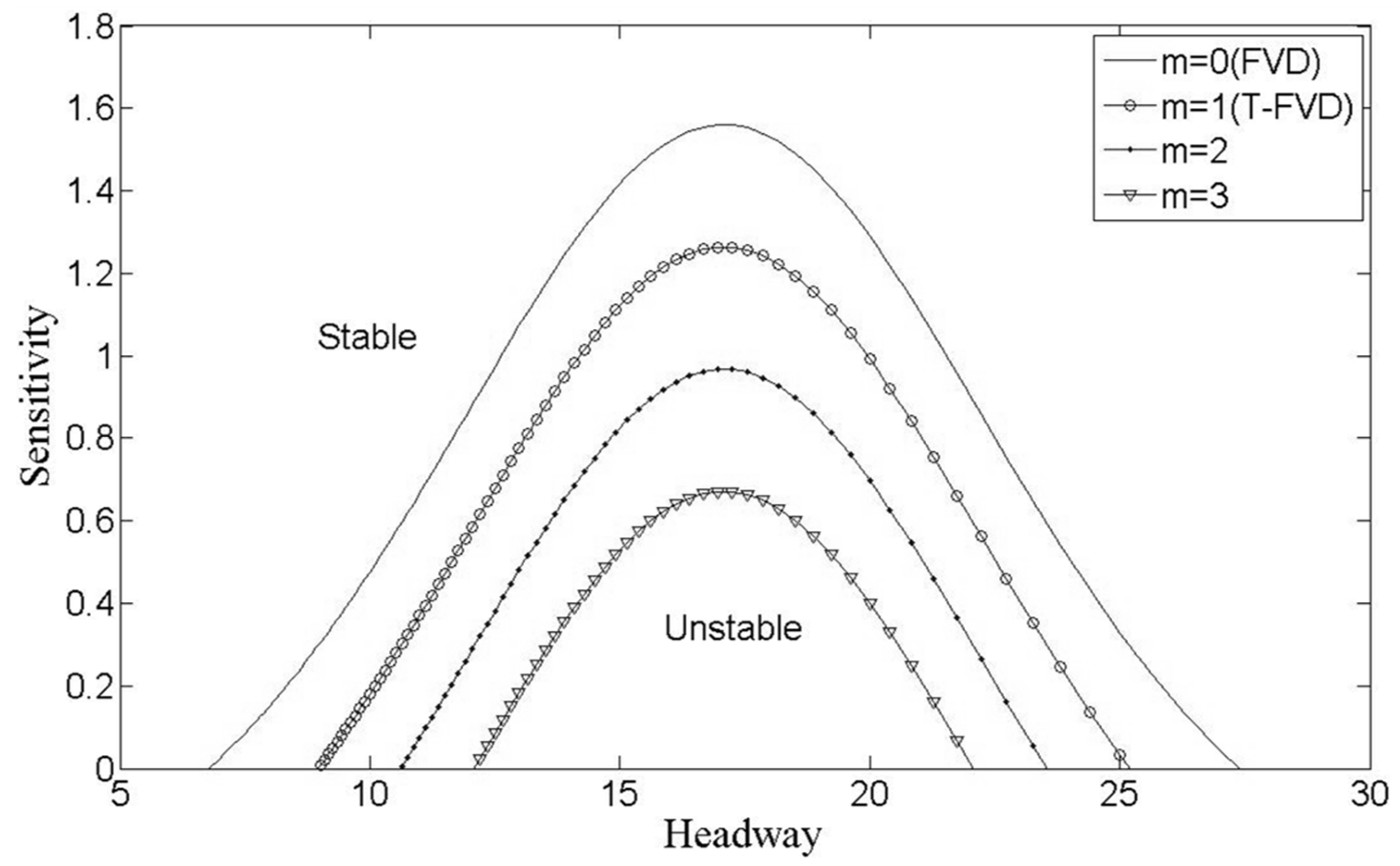
Figure 1 illustrates the neutral stability curves of the new model for different values of m, with , , and . The neutral stability curve divides the vehicle headway sensitivity phase space into two regions: the stable region above and the unstable region below. From Figure 1, it can be observed that as the control parameter m increases, which corresponds to collecting more average electronic throttle opening information from preceding vehicles in the CAV platoon control system, the stability region expands gradually. This indicates that by fully utilizing the average electronic throttle opening information of the preceding vehicle group, the downstream traffic flow trend can be effectively perceived, leading to improved stability of the CAV platoon control system. When m = 1, the critical stability curve obtained is consistent with the T-FVD model [29]. When m = 0, which means the absence of electronic throttle control signals from the preceding CAVs, the critical stability curve obtained is consistent with the FVD model.
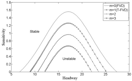
Figure 1.
The neutral stability curves in headway sensitivity space ().
3. Traffic Fuel Consumption and Emission Assessment Model
Fuel consumption and emissions, as external attributes of the transportation system, are strongly correlated with the inherent attribute of traffic flow stability. Recently, some scholars have begun to use the car-following theory to study the energy cons. For example, a unique periodic intermittent cruise controller was devised by Zhai et al. [36] with the goal of tracking and assessing, in real time, the operational state of road vehicles and the environmental parameters related to them. They expertly used the FVD modeling framework in the controller to model and simulate the dynamic driving process of the car on the road. This innovative controller significantly improved vehicle safety tracking performance, reduced energy consumption, and reduced exhaust emissions after being validated in real-world scenarios. On the other hand, by adding a relative velocity term, Zhang et al. [37] expanded on the coupled map car-following model and suggested a discrete vehicle-following model. On the basis of this, they created a delayed feedback controller with the goal of successfully reducing emissions and traffic congestion. The findings of this study offer fresh concepts and approaches for enhancing traffic dynamics and lowering pollution levels in the environment. In this section, the VT-Micro model [38] is introduced to elucidate the impact of the feedback control signal of the average electronic throttle opening of multiple preceding vehicles on fuel consumption and emission factors in the transportation system. Based on the instantaneous velocity and acceleration of vehicles, the VT-Micro model calculates the instantaneous emission factor of a vehicle at the current time, which is formulated as follows [38]:
where represents the vehicle velocity exponent, represents the vehicle acceleration exponent, and denotes the model regression coefficients corresponding to the velocity exponent and acceleration exponent . Equation (16) establishes the theoretical foundation for quantifying traffic emissions from vehicle microsimulation trajectory data. By setting the regression coefficients to different parameter values, as shown in Table 1 [38], the emission factors for CO, HC, NOX, and fuel consumption in the traffic system can be calculated. Based on Equation (16), the average emission rates of CO, HC, NOX, and fuel consumption per vehicle in the road traffic system can be further determined, as expressed by the following formula:
where represents the average emission factor (CO, HC, NOX, and fuel consumption) per vehicle per unit time in the road system, is the total number of vehicles in the road system, denotes the relaxation time, and represents the statistical time duration.

Table 1.
The corresponding values of fuel consumption, CO emission, HC emission and NOX emission in VT-Micro model [38].
According to the working principle of the VT-Micro model [38], by inputting the velocity and acceleration data of the vehicle at each simulation time step, the corresponding fuel consumption and transportation emission levels of the vehicle can be calculated. Therefore, first, we need to conduct numerical simulation experiments using the proposed CAV vehicle dynamics model in Equation (6) to obtain the vehicle trajectory data at each time step. The Euler method is utilized in the numerical simulation to obtain an approximate solution to Equation (6). The corresponding iterative time step is set as h = 0.01.
4. Simulation Analysis
To analyze the stability and spatio-temporal evolution mechanism of the CAV cruise control system in terms of the average electronic throttle opening information of multiple preceding vehicles, numerical simulations are conducted based on the proposed model under periodic boundary conditions. For this purpose, N CAV vehicles are evenly distributed on a circular road with length L. It is assumed that the leading vehicle experiences external perturbation signals at the initial time [29]:
The simulation input parameters are as follows: , , , , , , .
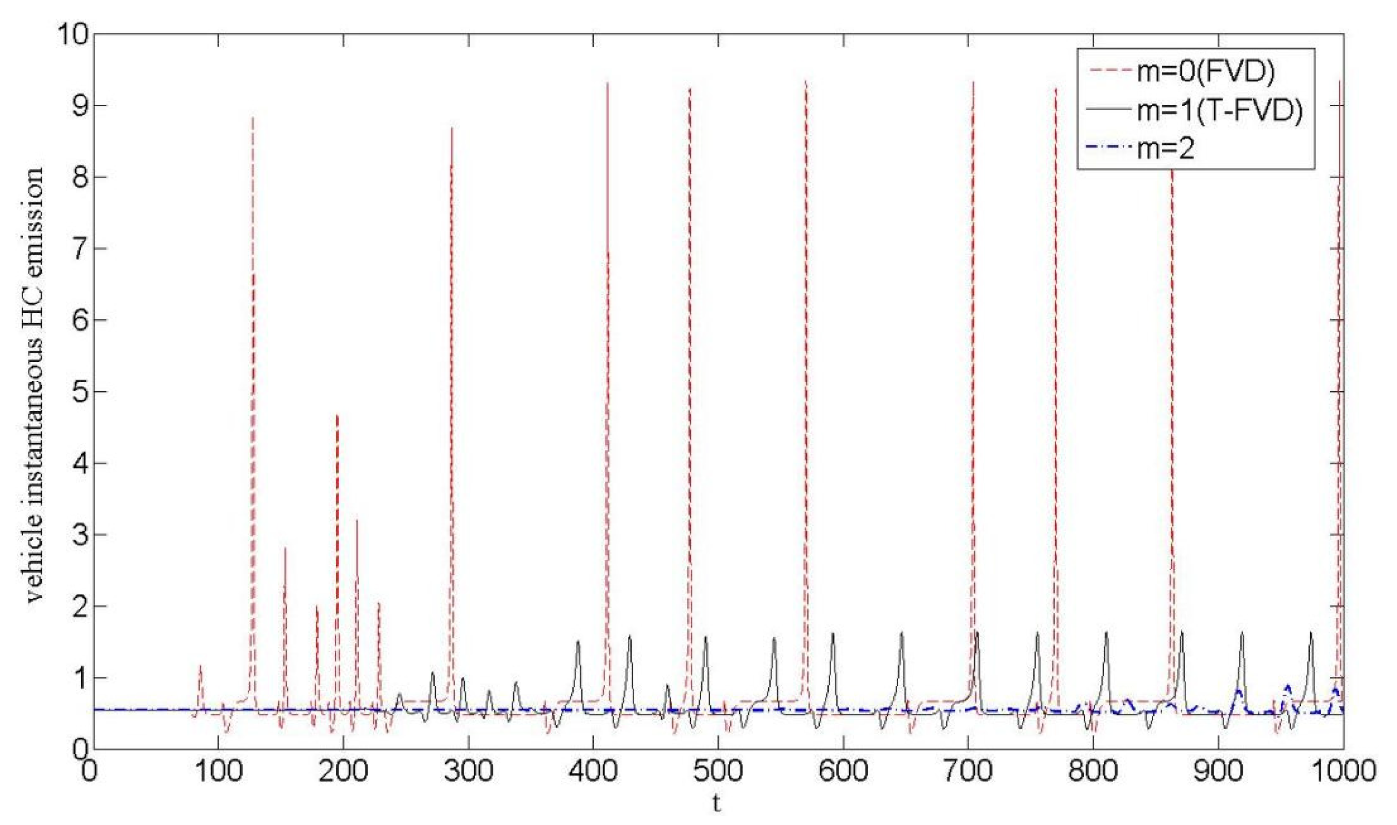
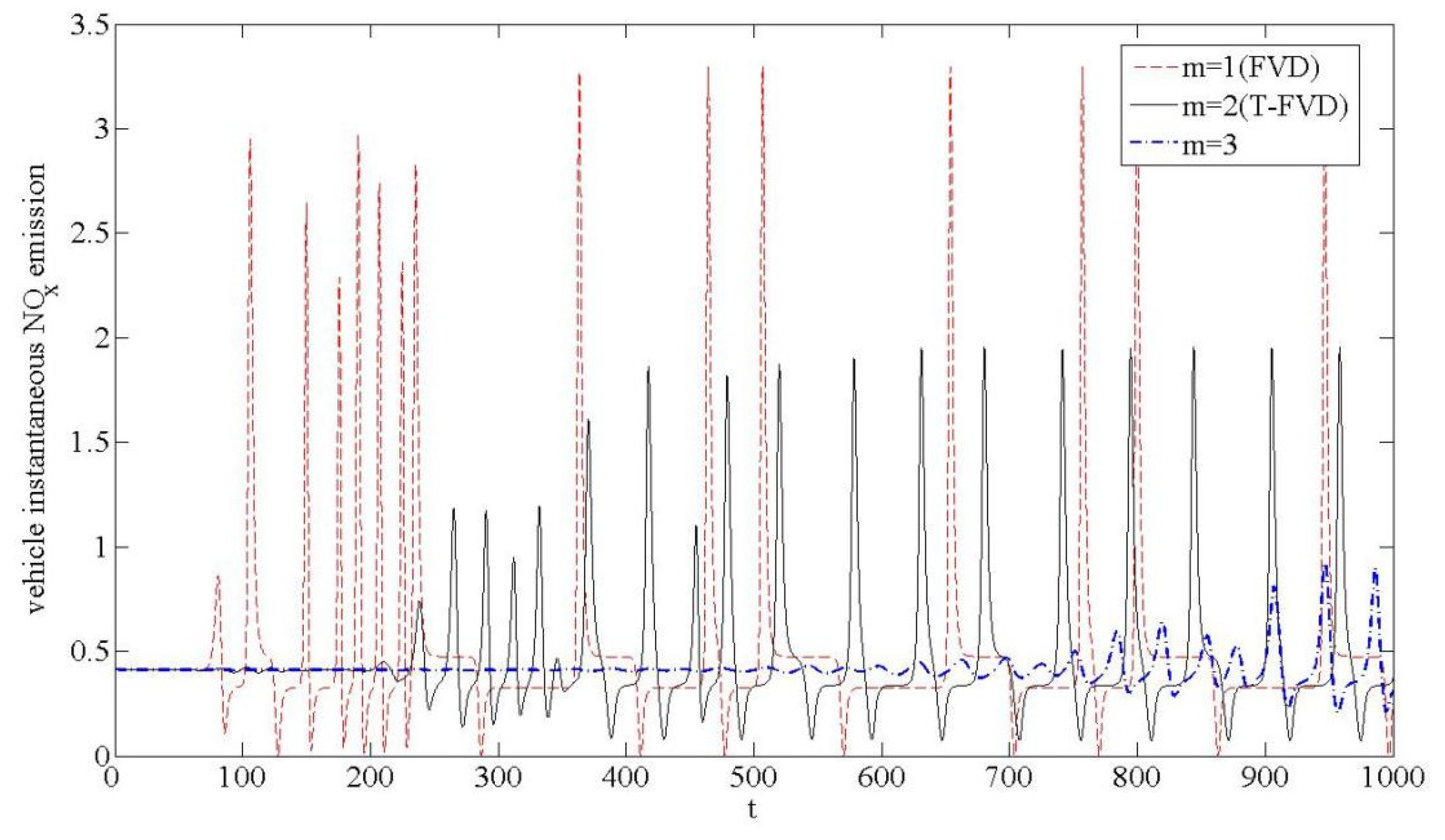
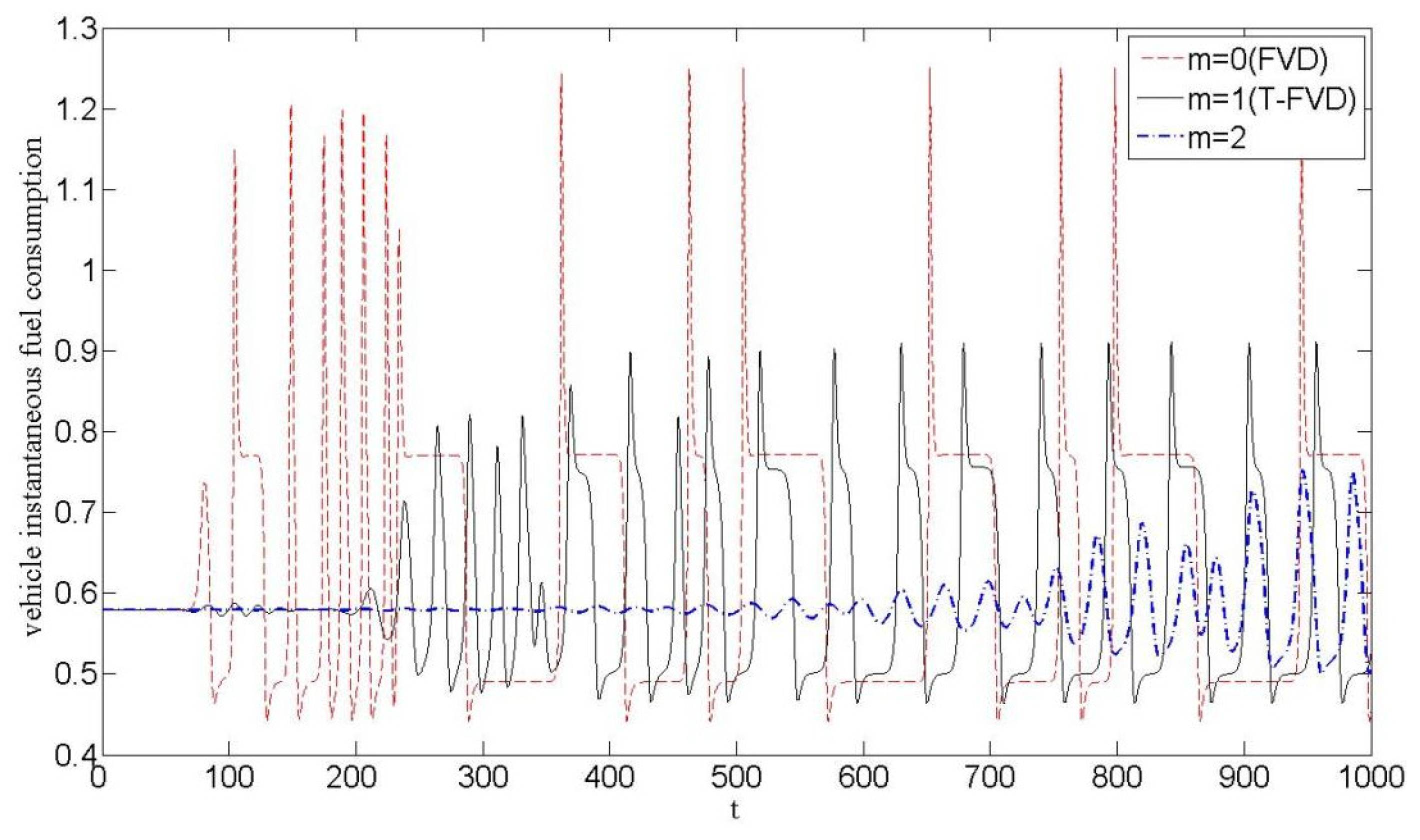
In the scenario of traffic flow perturbation described by Equations (18) and (19), the CAV platoon on the circular road will experience speed oscillations. These oscillations will have an impact on the stability of the CAV platoon and the associated instantaneous emission factors (CO, HC, NOX, and fuel consumption). Based on the calculation (Formula (16)) of the VT-Micro model, the evolution patterns of the emission factors (CO, HC, NOX, and fuel consumption) can be obtained. Figure 2, Figure 3, Figure 4 and Figure 5 reveal the temporal evolution of individual vehicle’s instantaneous emission factors (CO, HC, NOX, and fuel consumption) with respect to the control parameter under different values.
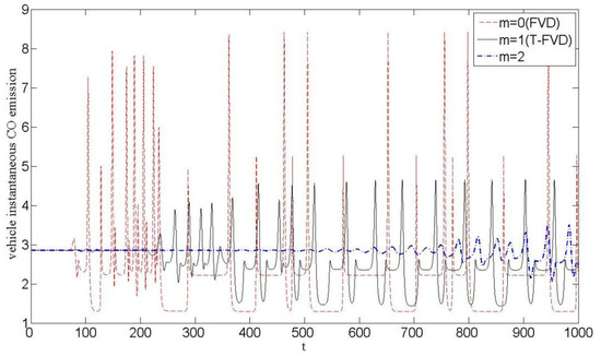
Figure 2.
The relationship between vehicle instantaneous CO emission and time t under different values m.
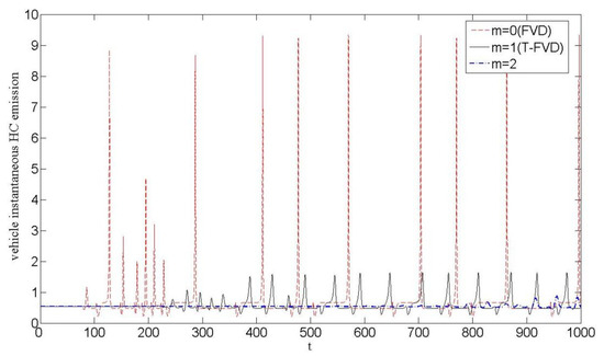
Figure 3.
The relationship between vehicle instantaneous HC emission and time t under different values m.
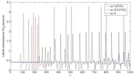
Figure 4.
The relationship between vehicle instantaneous NOX emission and time t under different values m.
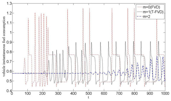
Figure 5.
The relationship between fuel consumption and time t under different values m.
From Figure 2, Figure 3, Figure 4 and Figure 5, it can be observed that the number of CAV vehicles (m) providing electronic throttle angle information in the proposed cruise control model has a significant impact on the emission factors (CO, HC, NOX, and fuel consumption) of the vehicles. When m = 0, corresponding to the FVD model where electronic throttle control signals are not considered, the instantaneous emission factors (CO, HC, NOX, and fuel consumption) of the vehicles exhibit significant fluctuations. On the other hand, when m = 1, corresponding to the T-FVD model where electronic throttle angle control signals are introduced, the stability of vehicle operations improves, leading to a noticeable reduction in the fluctuation in the instantaneous emission factors. Furthermore, as the value of m increases, the stability of vehicle operations further improves, resulting in enhanced suppression of fluctuations in the instantaneous emission factors (CO, HC, NOX, and fuel consumption), with the corresponding variation range gradually narrowing and approaching stability.
In conclusion, considering the average electronic throttle angle control information of the preceding vehicle queue during the CAV platoon cruise control process plays a significant role in improving traffic flow performance and stabilizing the instantaneous emission levels of CAV vehicles. This observation is consistent with the stability analysis results shown in Figure 1.
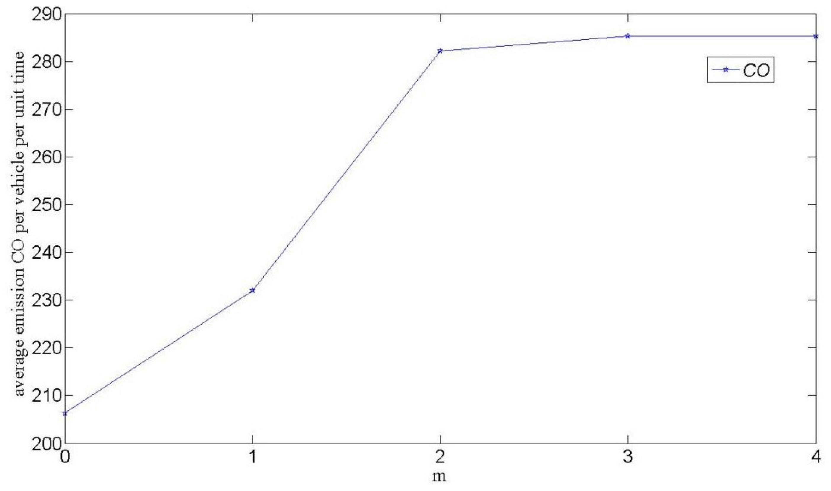
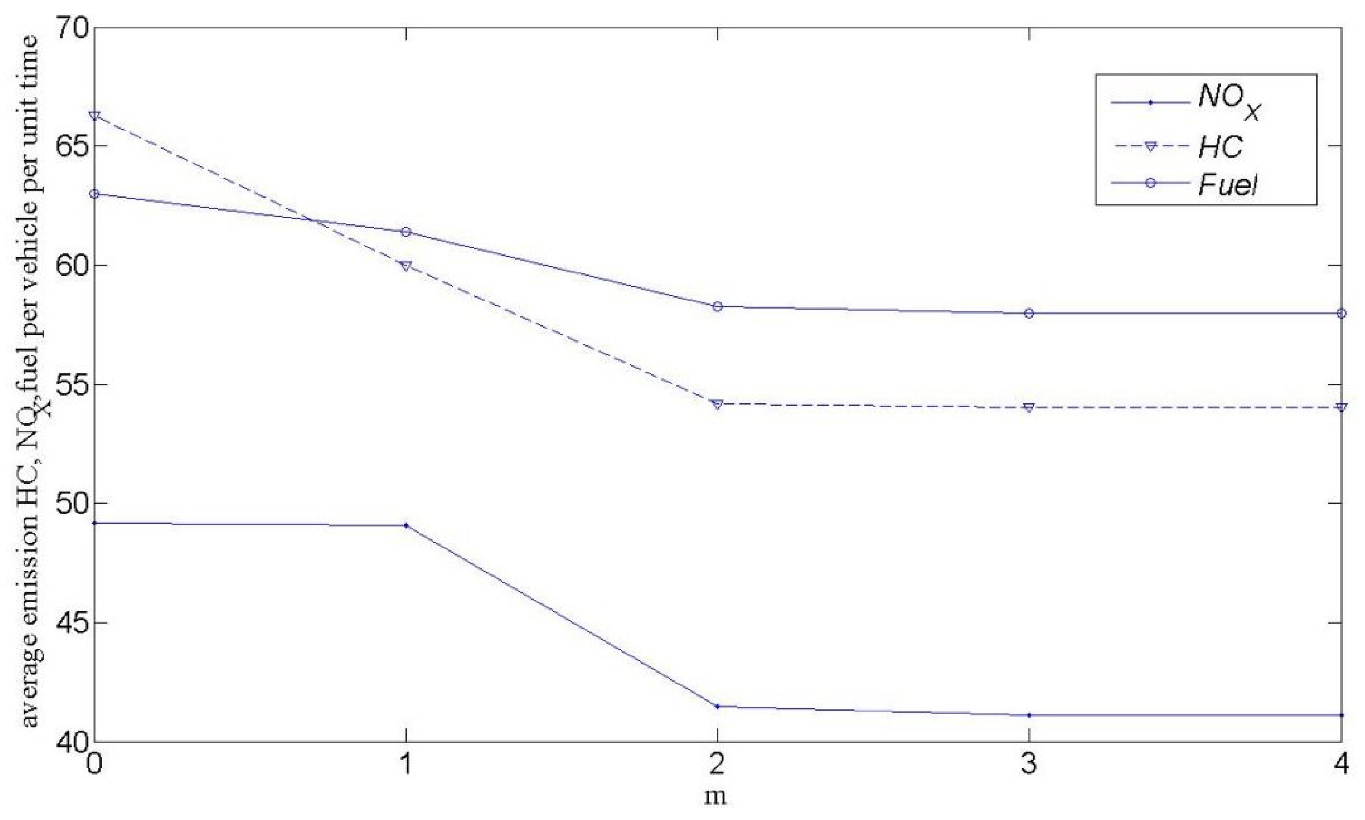
To analyze the evolutionary mechanism of the overall emission factors in the road system, we utilize Equation (17) to calculate the average emission factors (CO, HC, NOX, and fuel consumption) of all vehicles during the statistical period. To eliminate transient effects, a relaxation time of t0 = 700 and a statistical time step of T = 100 are used in Equation (17). The simulation results are shown in Figure 6 and Figure 7. Figure 6 and Figure 7 present the average release levels per vehicle per unit time of CO, HC, NOX, and fuel consumption in the road system for different values of the control parameter m. It can be observed that in Figure 7, the average release levels of HC, NOX, and fuel consumption per vehicle per unit time gradually decrease as the control parameter m increases. This indicates that in the CAV platoon cruise control system, utilizing the electronic throttle feedback signals from the preceding vehicles can effectively improve the average emission levels of HC, NOX, and fuel consumption in the traffic system, which is of significant importance for the development of environmentally friendly transportation. However, Figure 6 reveals a distinct phenomenon where the average release level of CO per vehicle per unit time gradually increases as the parameter m increases. This suggests that the improvement in traffic system stability does not necessarily correspond to an improvement in the average emission level of CO. Nevertheless, from the evolutionary trends of the unit-time emission levels of CO, HC, NOX, and fuel consumption shown in Figure 6 and Figure 7, it can be observed that when the control parameter m is set to 3 in the CAV platoon cruise control system, the curves for CO, HC, NOX, and fuel consumption become horizontal lines. This indicates that considering the average electronic throttle angle control information of the preceding three vehicles in the networked cruise control model can enable the traffic system to achieve an optimal operating state, with the corresponding emission factors (CO, HC, NOX, and fuel consumption) reaching a relatively stable release level.
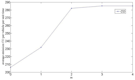
Figure 6.
The change in CO for presented model at different values of m.
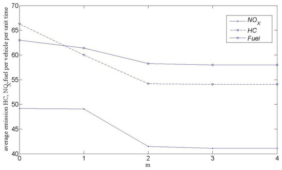
Figure 7.
The change in HC, NOX and fuel consumption emissions for presented model at different values of m.
In summary, we can draw the following conclusions:
(1) By combining the traffic following model with empirical emission formulations, we are able to accurately capture and simulate the evolution of vehicle emissions under different traffic conditions. This method provides a powerful tool for real-time monitoring and assessment of roadway emission levels and helps us to more accurately capture and predict the environmental impacts of transportation systems. However, it should be emphasized that this method needs to calibrate the parameters of the model with specific traffic scenarios in practical applications.
(2) The introduction of a feedback mechanism based on the average information of the electronic throttle opening of the vehicle population on the downstream roadway in the CAV vehicle networked cruise control modeling mode not only significantly improves the stability of the traffic flow but also achieves significant reductions in fuel consumption and emissions of pollutants, such as CO, HC, and NOX. This innovative technology not only optimizes traffic efficiency but also shows certain potential and value in energy savings and emission reduction, which is of great significance for building a sustainable transportation system.
5. Conclusions
In the context of vehicular networking, intelligent connected and automated vehicles (CAVs) equipped with vehicle-to-vehicle communication and real-time traffic sensing technologies can capture downstream traffic trends over a wider range and form a networked cruise control system with the monitored preceding CAV platoon. In this study, we proposed a new CAV platoon cruise control model for the application scenario of CAV platoons by incorporating the average feedback signal of electronic throttle angles from preceding vehicles. Under periodic boundary conditions, the linear stability conditions of the model under small perturbation signal interference are derived using linear stability theory. From the perspective of evaluating emission levels (CO, HC, NOX, and fuel consumption), the impact of the number of CAV vehicles in the average feedback signal of electronic throttle angles on the instantaneous emission factors of individual vehicles and the average release intensity of collective emission factors on the road is systematically studied. The research results demonstrate that in the cruise control strategy, as the number of CAV vehicles included in the average feedback signal of electronic throttle angles increases, the traffic flow stability improves, and the fluctuation level of associated instantaneous emission factors (CO, HC, NOX, and fuel consumption) of individual vehicles decreases significantly, maintaining a relatively stable emission level. The calculation results of the average emission levels of collective emission factors for CAV platoons indicate that collecting the average electronic throttle angle control information of more preceding vehicles leads to a significant reduction in HC, NOX, and fuel consumption emissions, but the average CO emission level gradually increases. Specifically, when the number of CAV vehicles providing feedback signals is set to 3, the CO, HC, NOX, and fuel consumption levels of the CAV platoon reach a steady state. In summary, the CAV platoon cruise control system constructed based on the average feedback signal of electronic throttle angles from the preceding vehicle platoon can effectively enhance the traffic flow stability and significantly improve the CO, HC, NOX, and fuel consumption emissions at both the individual instantaneous level and the average statistical level of the platoon.
The model results provide an important reference for transportation planners and automobile manufacturers in designing and optimizing the control strategies of transportation systems in order to reduce traffic congestion, smooth the vehicle movement process, and, thus, reduce the overall energy consumption and emissions of the transportation system. However, the current work is mainly based on vehicle trajectory data obtained from numerical simulations, and although this provides valuable insights for studying the energy consumption and emissions during the car-following process, there are still some limitations. In future work, we plan to collect field data to test the model performance in order to obtain more accurate and practical control strategies.
Author Contributions
Validation, C.T.; methodology, Y.K.; writing—original draft, C.T.; writing—review & editing, Y.K.; supervision, Y.K.; funding acquisition, Y.K. All authors have read and agreed to the published version of the manuscript.
Funding
This research was funded by Guizhou Institute of technology high-level talent research start-up funding project.
Data Availability Statement
The original contributions presented in the study are included in the article, further inquiries can be directed to the corresponding author.
Acknowledgments
This paper was supported by the Guizhou Institute of technology high-level talent research start-up funding project.
Conflicts of Interest
The authors declare no conflicts of interest.
Abbreviations
| CAVs | Connected and automated vehicles |
| CO | Carbon Monoxide |
| HC | Hydrocarbon |
| NOx | Oxides of Nitrogen |
| FVD | Full Velocity Difference |
| T-FVD | Throttle-based FVD |
| ET | Electronic throttle |
| IVC | Inter-vehicle communication |
| OV | Optimal Velocity |
References
- Kuang, H.; Wang, M.T.; Lu, F.H.; Bai, K.Z.; Li, X.L. An extended car-following model considering multi-anticipative average velocity effect under V2V environment. Physical A 2019, 527, 121268. [Google Scholar] [CrossRef]
- Lenz, H.; Wagner, C.; Sollacher, R. Multi-anticipative car-following model. Eur. Phys. J. B 1999, 7, 331–335. [Google Scholar] [CrossRef]
- Ge, H.X.; Zhu, H.B.; Dai, S.Q. Effect of looking backward on traffic flow in a cooperative driving car following model. Eur. Phys. J. B 2006, 54, 503–507. [Google Scholar] [CrossRef]
- Ma, M.H.; Xiao, J.H.; Liang, S.D.; Hou, J.J. An extended car-following model accounting for average optimal velocity difference and backward-looking effect based on the Internet of Vehicles environment. Mod. Phys. Lett. B 2022, 36, 2150562. [Google Scholar] [CrossRef]
- Nakayama, A.; Sugiyama, Y.; Hasebe, K. Effect of looking at the car that follows in an optimal velocity model of traffic flow. Phys. Rev. E 2002, 65, 016112. [Google Scholar] [CrossRef]
- Ge, H.X.; Dai, S.Q.; Xue, Y.; Dong, L.Y. Stabilization analysis and modified Korteweg-de Vries equation in a cooperative driving system. Phys. Rev. E 2005, 71 Pt 2, 066119. [Google Scholar] [CrossRef]
- Wang, T.; Gao, Z.Y.; Zhao, X.M. Multiple velocity difference model and its stability analysis. Acta Phys. Sin. 2006, 55, 634–640. [Google Scholar] [CrossRef]
- Yu, L.; Shi, Z.; Zhou, B. Kink-antikink density wave of an extended car following model in a cooperative driving system. Commun. Nonlinear Sci. Numer. Simul. 2008, 13, 2167–2176. [Google Scholar] [CrossRef]
- Sun, D.H.; Kang, Y.R.; Yang, S.H. A novel car following model considering average speed of preceding vehicles group. Physical A 2015, 436, 103–109. [Google Scholar] [CrossRef]
- Zhai, C.; Wu, W.T. Self-delayed feedback car-following control with the velocity uncertainty of preceding vehicles on gradient roads. Nonlinear Dyn. 2021, 106, 3379–3400. [Google Scholar] [CrossRef]
- Sun, D.H.; Zhang, J.C.; Liao, X.Y.; Tian, C.; Li, Y.F.; Liu, W.N. Optimal velocity difference model of non-neighboring vehicles. J. Traffic Transp. Eng. 2011, 11, 114–118. [Google Scholar]
- Wu, B.; Wang, W.X.; Li, L.B.; Liu, Y.T. Longitudinal control model for connected autonomous vehicles influenced by multiple preceding vehicles. J. Traffic Transp. Eng. 2020, 20, 184–194. [Google Scholar]
- Tang, T.Q.; Shi, W.F.; Shang, H.Y.; Wang, P.Y. An extended car-following model with consideration of the reliability of inter-vehicle communication. Measurement 2014, 58, 286–293. [Google Scholar] [CrossRef]
- Zhang, L.D.; Zhang, M.M.; Wang, J.; Li, X.W.; Zhu, W.X. Internet connected vehicle platoon system modeling and linear stability analysis. Comput. Commun. 2021, 174, 92–100. [Google Scholar] [CrossRef]
- Hossain, M.A.; Tanimoto, J. A microscopic traffic flow model for sharing information from a vehicle to vehicle by considering system time delay effect. Physical A 2022, 585, 126437. [Google Scholar] [CrossRef]
- Li, Y.F.; He, C.P.; Zhu, H.; Zheng, T.X. Nonlinear longitudinal control for heterogeneous connected vehicle platoon in the presence of communication delays. Acta Autom. Sin. 2021, 47, 2841–2856. [Google Scholar]
- Bando, M.; Hasebe, K.; Nakayama, A.; Shibata, A.; Sugiyama, Y. Dynamical model of traffic congestion and numerical simulation. Phys. Rev. E 1995, 51, 1035–1042. [Google Scholar] [CrossRef] [PubMed]
- Jiang, R.; Wu, Q.S.; Zhu, Z.J. Full velocity difference model for a car following theory. Phys. Rev. 2001, 64, 017101-1. [Google Scholar] [CrossRef] [PubMed]
- Wang, X.; Xue, Y.; Cen, B.L.; Zhang, P.; He, H.D. Study on pollutant emissions of mixed traffic flow in cellular automaton. Physical A 2020, 537, 122686. [Google Scholar] [CrossRef]
- Liu, Z.Z.; Cheng, R.J.; Ge, H.X. Research on preceding vehicle’s taillight effect and energy consumption in an extended macro traffic model. Physical A 2019, 525, 304–314. [Google Scholar]
- Peng, G.H.; Jia, T.T.; Kuang, H.; Tan, H.L. Energy consumption in a new lattice hydrodynamic model based on the delayed effect of collaborative information transmission under V2X environment. Physical A 2022, 585, 126443. [Google Scholar] [CrossRef]
- Jin, Z.Z.; Yang, Z.L.; Ge, H.X. Energy consumption investigation for a new car-following model considering driver’s memory and average speed of the vehicles. Physical A 2018, 506, 1038–1049. [Google Scholar] [CrossRef]
- Huang, L.; Zhai, C.; Wang, H.W.; Zhang, R.H.; Qiu, Z.J.; Wu, J.P. Cooperative Adaptive Cruise Control and exhaust emission evaluation under heterogeneous connected vehicle network environment in urban city. J. Environ. Manag. 2020, 256, 109975. [Google Scholar] [CrossRef] [PubMed]
- Guo, X.Y.; Zhang, G.; Jia, A.F. Stability and energy consumption of a double flow controlled two-lane traffic system with vehicle-to-infrastructure communication. Appl. Math. Model. 2023, 120, 98–114. [Google Scholar] [CrossRef]
- Li, Z.P.; Chen, L.Z.; Xu, S.Z.; Qian, Y.Q. Analytical studies of CO2 emission in a mixed traffic flow with different vehicles. Physical A 2014, 413, 320–328. [Google Scholar] [CrossRef]
- He, H.D.; Zhang, C.G.; Wang, W.L.; Hao, Y.Y.; Ding, Y. Feedback control scheme for traffic jam and energy consumption based on two-lane traffic flow model. Transp. Res. Part D 2018, 60, 76–84. [Google Scholar] [CrossRef]
- Tang, T.Q.; Huang, H.J.; Shang, H.Y. Influences of the driver’s bounded rationality on micro driving behavior, fuel consumption and emissions. Transp. Res. Part D 2015, 41, 423–432. [Google Scholar] [CrossRef]
- Yao, Z.H.; Wang, Y.; Liu, B.; Zhao, B.; Jiang, Y.S. Fuel consumption and transportation emissions evaluation of mixed traffic flow with connected automated vehicles and human-driven vehicles on expressway. Energy 2021, 230, 120766. [Google Scholar] [CrossRef]
- Li, Y.F.; Zhang, L.; Peeta, S.; He, X.Z.; Zheng, T.X.; Li, Y.G. A car-following model considering the effect of electronic throttle opening angle under connected environment. Nonlinear Dyn. 2016, 85, 2115–2125. [Google Scholar] [CrossRef]
- Li, Y.F.; Yang, H.; Yang, B.; Zheng, T.X.; Zhang, C. An extended continuum model incorporating the electronic throttle dynamics for traffic flow. Nonlinear Dyn. 2018, 93, 1923–1931. [Google Scholar] [CrossRef]
- Qin, Y.Y.; Wang, H.; Ran, B. Car-following model of connected and autonomous vehicles considering multiple feedbacks. J. Transp. Syst. Eng. Inf. Technol. 2018, 18, 48–54. [Google Scholar]
- Yan, C.Y.; Ge, H.X.; Cheng, R.J. An extended car-following model by considering the optimal velocity difference and electronic throttle angle. Physical A 2019, 535, 122216. [Google Scholar] [CrossRef]
- Sun, Y.Q.; Ge, H.X.; Cheng, R.J. A car-following model considering the effect of electronic throttle opening angle over the curved road. Physical A 2019, 534, 122377. [Google Scholar] [CrossRef]
- Zhai, C.; Wu, W.T.; Xiao, Y.P. Cooperative car-following control with electronic throttle and perceived headway errors on gyroidal roads. Appl. Math. Model. 2022, 108, 770–786. [Google Scholar] [CrossRef]
- Helbing, D.; Tilch, B. Generalized force model of traffic dynamics. Phys. Rev. E 1998, 58, 133–138. [Google Scholar] [CrossRef]
- Zhai, C.; Xu, Y.Q.; Li, K.N.; Zhang, R.H.; Peng, T.; Zong, C.F. Periodic intermittent cruise control: An innovative approach for reducing fuel consumption and exhaust emissions in road traffic systems. Process Saf. Environ. Prot. 2023, 177, 1197–1210. [Google Scholar] [CrossRef]
- Zhang, L.D.; Zhu, W.X. Delay-feedback control strategy for reducing CO2 emission of traffic flow system. Physical A 2015, 428, 481–492. [Google Scholar] [CrossRef]
- Ahn, K.; Rakha, H.; Trani, A.; Van Aerde, M. Estimating Vehicle Fuel Consumption and Emissions Based on Instantaneous Speed and Acceleration Levels. J. Transp. Eng. 2002, 128, 182–190. [Google Scholar] [CrossRef]

Disclaimer/Publisher’s Note: The statements, opinions and data contained in all publications are solely those of the individual author(s) and contributor(s) and not of MDPI and/or the editor(s). MDPI and/or the editor(s) disclaim responsibility for any injury to people or property resulting from any ideas, methods, instructions or products referred to in the content. |
© 2024 by the authors. Licensee MDPI, Basel, Switzerland. This article is an open access article distributed under the terms and conditions of the Creative Commons Attribution (CC BY) license (https://creativecommons.org/licenses/by/4.0/).