A Scalable Joint Estimation Algorithm for SOC and SOH of All Individual Cells within the Battery Pack and Its HIL Implementation

Abstract

Accurately obtaining the state of charge (SOC) and health (SOH) of all individual batteries in a battery pack can provide support for data acquisition, state estimation, and fault diagnosis. To verify the real-time performance and accuracy of the joint estimation algorithm for high-voltage battery packs composed of 96 individual cells in series, this article applies Simulink to develop a joint estimation algorithm for SOC and SOH based on the first-order RC equivalent circuit model (1RC ECM) and implements the algorithm’s cyclic calling for series nodes, enhancing the algorithm’s scalability. In the algorithm, the recursive least square method with fitting factor (FFRLS) is applied to calculate OCV, R₀, and R₁ in the time domain, and dual adaptive extended Kalman filter (DAEKF) is applied to joint estimation of SOC and SOH at multiple time scales. Finally, with the help of dSPACE and FASECU controllers, hardware in the loop (HIL) testing was completed in multiple scenarios. The results showed that the algorithm can accurately calculate the state of individual cells in real time, and even under various initial value deviations, it still has good regression performance, laying the foundation for future applications of electric vehicles.

1. Introduction

Lithium batteries are the main energy supply components of new energy vehicles, with the advantages of fast charging, high energy density, and light weight [1,2]. The accurate estimation of the state of the lithium battery is related to the reliability and safety of the vehicle. At present, most studies on battery state estimation focus on battery state of charge (SOC) and battery state of health (SOH). The former can monitor the battery’s charge to avoid overcharge and over-discharge, and the latter can monitor the aging state of the battery to determine the maintenance and replacement time of the battery, which can improve the safety of the battery. There is a coupling relationship between the two states; if we conduct research only for one state, it will lead to a reduction in the accuracy of the estimation results [3,4]. Therefore, the joint estimation of SOC and SOH provides a good solution to the problem of battery state estimation.

Considering the coupling relationship between SOC and SOH, SOC and SOH are estimated simultaneously by several filtering algorithms. GuoF et al. [5] proposed a multi-time scale SOC and parameter estimation method based on double Kalman filters and adjusted the parameters of double extended Kalman filters in joint estimation by means of empirical tuning. ShuzhiZ et al. [6] proposed a joint capacity and SOC estimation framework based on a dual adaptive extended Kalman filter (AEKF). The model parameters are obtained online by the recursive least square method with forgetting factor (FFRLS), and then the SOC and capacity are estimated jointly by two AEKF estimators. The joint estimation algorithm can better deal with the coupling relationship between SOC and SOH estimation, improve the accuracy of two-state estimation, and has a good application prospect. Battery model parameters are the key factors that affect the effect of battery state estimation. Model parameters are mainly obtained through offline parameter identification and online parameter identification, and offline parameters are obtained through hybrid power pulse test (HPPC) identification under laboratory conditions [7]. This method has good stability, but the test cost is high, and the parameter accuracy is poor when there are errors in the battery state. Online parameter model parameter values [8,9] are calculated in real time by the online identification algorithm. When battery temperature and aging state are unknown, model parameters can still be identified more accurately, with strong adaptability. DaiH et al. [10] proposed a multi-time-scale extended Kalman filter that considered the fast-slow variation characteristics of battery parameters and carried out parameter identification on different time scales, with reliable parameter identification results and high precision. It can be seen that it is necessary to identify model parameters according to battery variation characteristics.

For a battery pack composed of hundreds of individual batteries in series, due to the different decay trajectories of each battery, it is necessary to find a method to determine the SOC of all individual batteries in the series battery pack, in order to provide support for battery balance control and tracking of decay trajectories from the perspective of model parameters. Plett [11] explored a cute method called “bar-delta filtering” that took advantage of the fundamental similarity between all series connected cells in a pack and could estimate the SOC, resistance, and capacity of each cell in a manner requiring only somewhat more computational effort than for a single cell. Enlightened by [11], a method enabling cell-specific state estimation is studied in [12]. This method is developed based on an extended Kalman filter (EKF) and an equivalent circuit model. The method uses the current and “averaged cell” voltage to determine the battery pack’s average SOC at first and thereafter incorporates the performance divergence between the “averaged cell” and each individual cell to generate the SOC estimation for all cells. To reduce the computation cost, a dual time-scale implementation is designed. The method is validated using results obtained from the measurements of a Li-ion battery pack. Due to the rigorous requirements on real-time and sampling synchronization, a controller area network (CAN)-based battery management system is also being developed to implement the method. To address the difficulty of state estimation by cell inconsistency and realize joint estimation of the state of charge (SOC) and capacity for series-connected battery packs, a novel cell-to-pack state estimation extension method based on a multilayer difference model (MDM) is investigated in [13]. The proposed extension method can efficiently realize accurate SOC and capacity estimation for a battery pack based on the existing estimation algorithms for a single cell. Two state-difference estimators for SOC and capacity differences are constructed and realized separately through the adaptive extended Kalman filter and the recursive least squares algorithm. Considering that time-varying characteristics of states and state differences are different, the MDM estimator runs in multiple timescales. Based on battery pack cycling experiments, the cell-to-cell consistency evolution during aging is revealed. The proposed MDM’s accuracy, efficiency, and adaptability are verified through the experiments of a series-connected battery pack under different dynamic conditions. The proposed method also shows adaptability to various battery temperatures and different cell inconsistencies.

In order to achieve an accurate joint estimation of SOC and SOH for each individual cell in the battery pack, the SOC deviation matrix established for each cell is used to fit and calculate the terminal voltage of each cell. It is necessary to run the AEKF of SOC difference on another time scale, which will undoubtedly increase the burden of parameter tuning and may not necessarily have a beneficial effect on ensuring algorithm estimation accuracy and reducing computational load. At present, there is little research on how to obtain real-time SOC and SOH of each individual cell in the entire battery pack through lightweight calculation and process variable storage. In this paper, a multi-time scale Kalman filter algorithm combining off-line parameter identification and on-line parameter identification is established to perform SOC and SOH joint estimation, ensuring the feasibility and computational accuracy of a set of algorithms at a determined time scale, and seeks methods to extend the flexible and scalable joint estimation algorithm to the cyclic calculation and HIL implementation of other cells within the battery pack.

The rest of this paper is as follows: In the second section, a joint SOC and SOH estimation scheme considering battery model parameters is proposed. In the third section, at the application layer level, Simulink was used to implement the SOC-SOH joint estimation algorithm and its cyclic call for 96 individual cells. In the fourth section, multi-scenarios HIL testing shows that the joint estimation algorithm proposed in this article for 96 cells has good real-time performance and precise computing power. In addition, the article is summarized in the last section.

2. SOC and SOH Joint Estimation Scheme and Pre-Data Processing

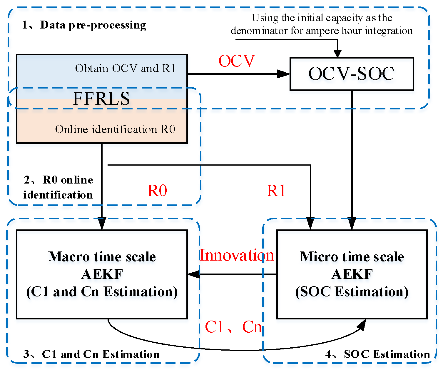
2.1. SOC and SOH Joint Estimation Scheme

SOC represents the remaining state of charge in the battery, and the calculation formula is shown in Equation (1), and SOH is defined as the ratio of the current actual capacity to the initial capacity, as shown in Equation (2).

$$\mathrm{S}\mathrm{O}\mathrm{C}=\frac{{\mathrm{C}}_{\mathrm{n}\_\mathrm{a}\mathrm{c}\mathrm{a}}}{{\mathrm{C}}_{\mathrm{n}\_\mathrm{a}\mathrm{c}\mathrm{t}}}$$

(1)

$$\mathrm{S}\mathrm{O}\mathrm{H}=\frac{{\mathrm{C}}_{\mathrm{n}\_\mathrm{a}\mathrm{c}\mathrm{t}}}{{\mathrm{C}}_{\mathrm{n}\_\mathrm{i}\mathrm{n}\mathrm{i}}}\times 100\mathrm{\%}$$

(2)

In Formulas (1) and (2), C_{n_aca} indicates the current available capacity of the battery; C_{n_act} indicates the actual capacity of the battery; and C_{n_ini} indicates the initial battery capacity.

In order to ensure the accuracy of SOC and SOH estimation, it is necessary to establish a reasonable battery model. Among the integer-order equivalent circuit models shown in [14,15], the first-order RC model has accuracy and low complexity, making it suitable for this research study. The first-order RC equivalent circuit model simulates the ohmic internal resistance through a resistance unit and the polarization process through an RC network, and its state-space equation is shown in the following equation:

$$\left\{\begin{array}{c}{\dot{\mathrm{U}}}_1(\mathrm{t})=\frac{\mathrm{I}\left(\mathrm{t}\right)}{{\mathrm{C}}_1}-\frac{{\mathrm{U}}_1\left(\mathrm{t}\right)}{{{\mathrm{R}}_1\mathrm{C}}_1}\\ {\mathrm{U}}_{\mathrm{t}}={\mathrm{U}}_{\mathrm{O}\mathrm{C}\mathrm{V}}+{\mathrm{U}}_1\left(\mathrm{t}\right)+\mathrm{I}{\left(\mathrm{t}\right)\mathrm{R}}_0\end{array}\right.$$

(3)

In the formula, U_OCV represents the open-circuit voltage of the battery without a load. U_t stands for terminal voltage; U₁ stands for polarization voltage; R₀ is ohmic internal resistance; and R₁ and C₁ are polarization parameters, representing polarization resistance and polarization capacitance, respectively. I indicate the load current, which is positive when charging and negative when discharging.

From the initial state of the SOC(0), the SOC calculation can be performed using the ampere hour integration method and the current at each time t, as follows:

$$\mathrm{S}\mathrm{O}\mathrm{C}=\mathrm{S}\mathrm{O}\mathrm{C}(0)-\frac{1}{{\mathrm{C}}_{\mathrm{n}\_\mathrm{a}\mathrm{c}\mathrm{t}}}{\int }_0^{\mathrm{t}}\mathrm{I}\left(\mathrm{t}\right)\mathrm{d}\mathrm{t}$$

(4)

In this paper, the joint estimation of SOC and SOH is realized through a multi-time-scale dual adaptive extended Kalman filter (DAEKF), and the implementation process of the scheme is shown in Figure 1. The main process of joint estimation is as follows: (1) The OCV-SOC relationship is constructed by the recurrent least square method with forgetting factor (FFRLS), and the polarization internal resistance R1 value is identified; (2) online identification of internal resistance R₀ by FFRLS; (3) capacity Cn and polarization capacitance C₁ are estimated by the AEKF algorithm at the macro-time scale; (4) SOC calculation is carried out by the AEKF algorithm at the micro-time scale. The identification of the OCV-SOC relationship curve and the polarization internal resistance R₁ is the preliminary data processing. The OCV identification under time series is carried out by FFRLS, and the corresponding relationship between the output OCV identification results and the SOC obtained by the ampt-hours integration method based on the nominal capacity is constructed into the high-order multivariate polynomial, which saves a lot of offline testing time. At the same time, the mean value of polarization resistance R₁ based on a first-order RC equivalent circuit at low current can be obtained and fixed, which will be used for subsequent multi-time-scale joint estimation algorithms accordingly. Further, the calculation of R₀ online parameter identification and SOC and SOH joint estimation is started. The internal resistance R₀ is calculated online by FFRLS, and the micro-time-scale SOC estimator is input for the calculation of terminal voltage prior to estimation. The update time is consistent with the micro-time-scale step. The macro-time-scale estimator is used to estimate C₁ and capacity, and the estimated results are input to the micro-time-scale SOC estimator for prior estimation of SOC and polarization voltage U₁. The micro-time-scale SOC estimator is used to estimate SOC and output the difference between the measured and the prior estimate of the terminal voltage, which is the new information, which will be put into the macro-time-scale estimator for C₁ and capacity estimation. The above is an overall overview of the SOC and SOH joint estimation algorithm.

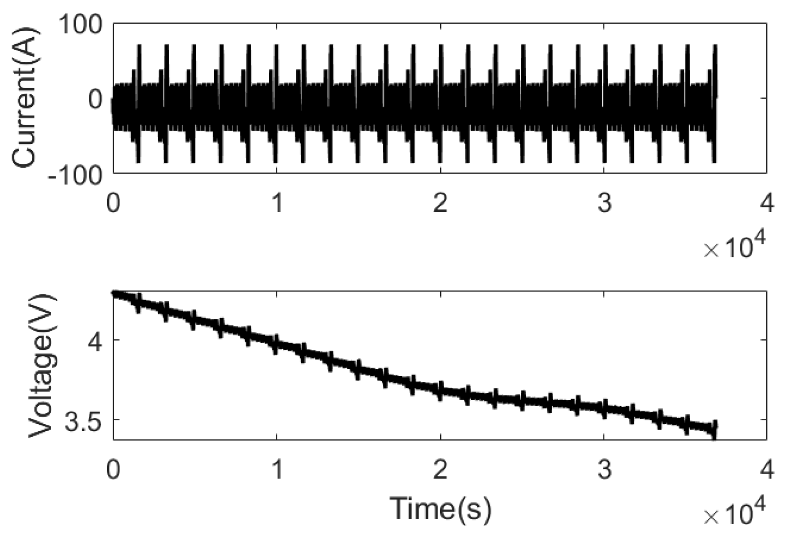
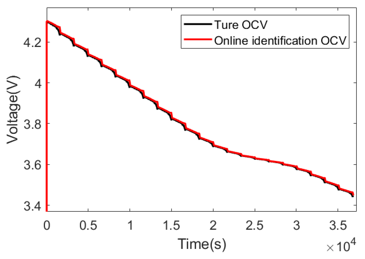
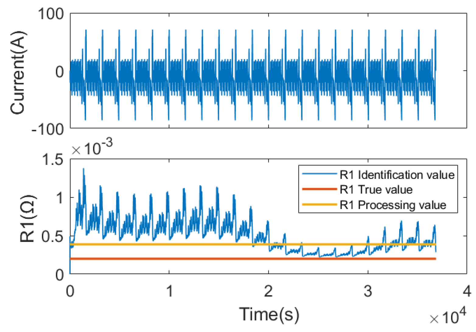
2.2. Early Data Processing Based on FFRLS to Obtain OCV, R1

The purpose of early data processing is to obtain a more accurate OCV-SOC correspondence and a fixed value of R₁ to reduce the difficulty of later parameter identification and improve the convergence speed of capacity identification results. Combined with the battery model, this part intends to obtain the online identification results of OCV and R₁, which are related to sampling time by the FFRLS algorithm. The FFRLS algorithm estimation R₀ module mainly includes four parts: Gain, coefficient update, covariance update, and parameter analysis. The calculation process is shown in the following pseudo code (Algorithm 1).

Algorithm 1: FFRLS to obtain OCV-SOC, R1 and R0

Input: ${\mathrm{U}}_{\mathrm{t}}\left(\mathrm{k}\right) ,$${\mathrm{U}}_{\mathrm{t}}(\mathrm{k}-1),\mathrm{I}\left(\mathrm{k}\right),\mathrm{I}(\mathrm{k}-1)$ Output: ${\mathrm{U}}_{\mathrm{O}\mathrm{C}\mathrm{V}},{\mathrm{R}}_1$, ${\mathrm{R}}_0$ // The calculation process of FFRLS // Parameter initialization    θ0, P0 for k = 1:N // Determine the input and parameter vectors $$\left\{\begin{array}{l}{\mathsf{\Phi }}_{\mathrm{k}}=\left({\mathrm{U}}_{\mathrm{t}}\right(\mathsf{k}-1), \mathsf{I}(\mathsf{k}), \mathsf{I}(\mathsf{k}-1), 1)\\ {\mathsf{\theta }}_{\mathrm{k}}=({\mathsf{\alpha }}_1, {\mathsf{\alpha }}_2, {\mathsf{\alpha }}_3, {\mathsf{\alpha }}_4)\hfill \end{array}\right.$$ (5) // Gain and error covariance calculation $$\left\{\begin{array}{l}{\mathrm{K}}_{\mathrm{k}}={\mathrm{P}}_{\mathrm{k}-1}{\mathsf{\Phi }}_{\mathrm{k}}^{\mathrm{T}}{(\mathsf{\lambda }-{\mathsf{\Phi }}_{\mathrm{k}}{\mathrm{P}}_{\mathrm{k}-1}{\mathsf{\Phi }}_{\mathrm{k}}^{\mathrm{T}})}^{-1}\\ {\mathrm{P}}_{\mathrm{k}}=\frac{1}{\mathsf{\lambda }}(\mathsf{I}-{\mathrm{K}}_{\mathrm{k}}{\mathsf{\Phi }}_{\mathrm{k}}){\mathrm{P}}_{\mathrm{k}-1}\end{array}\right.$$ (6) // Online parameter identification $$\left\{\begin{array}{l} {\mathsf{\epsilon }}_{\mathrm{k}}={\mathrm{z}}_{\mathrm{k}}-{\mathsf{\Phi }}_{\mathrm{k}}{\tilde{\mathsf{\theta }}}_{\mathrm{k}}\\ {\tilde{\mathsf{\theta }}}_{\mathrm{k}}={\tilde{\mathsf{\theta }}}_{\mathrm{k}-1}+{\mathrm{K}}_{\mathrm{k}}{\mathsf{\epsilon }}_{\mathrm{k}}\end{array}\right.$$ (7) end

In order to verify the accuracy of subsequent algorithms in identifying model parameters, the model parameters are set to constant values, which are: R₀ = 0.00065 Ω, R₁ = 0.0002 Ω, C₁ = 5000 F, C = 115 Ah, and T = 25 °C. By combining the equivalent circuit model of the 1RC, the measured current value under operating conditions is used as an excitation to calculate and output the terminal voltage of the cell. The current and cell voltage results are shown in Figure 2.

With the current and voltage in Figure 2 as inputs, OCV and R₁ are identified through FFRLS; the identification results of OCV are compared with the given OCV as shown in Figure 3, and the R₁ value is compared with the given R₁ value, as shown in Figure 4.

Because the current changes frequently in the operating condition, the identification results of FFRLS for different magnification currents are quite different, and the error between the identification results of polarization internal resistance and the real value is large at large magnification. Therefore, for the whole operating condition segment, the average value of R₁ at the low current of each segment is taken as the fixed value of R₁, and the calculation process is shown in the following equation. The fixed value of R₁ is output at the same time during the OCV construction process. In the actual application process, when the temperature is constant, R₁ is a fixed value. The R₁ processing value result line in Figure 4 is shown.

$${\mathrm{R}}_1=\mathrm{m}\mathrm{e}\mathrm{a}\mathrm{n}\left({\mathrm{R}}_1\right(\mathrm{m}\mathrm{i}\mathrm{n}\left({\mathrm{I}}_{\mathrm{h}}\right)\left)\right),\mathrm{h}=\mathrm{1,2}\dots \mathrm{n}$$

(8)

In the formula, n is the number of working condition segments.

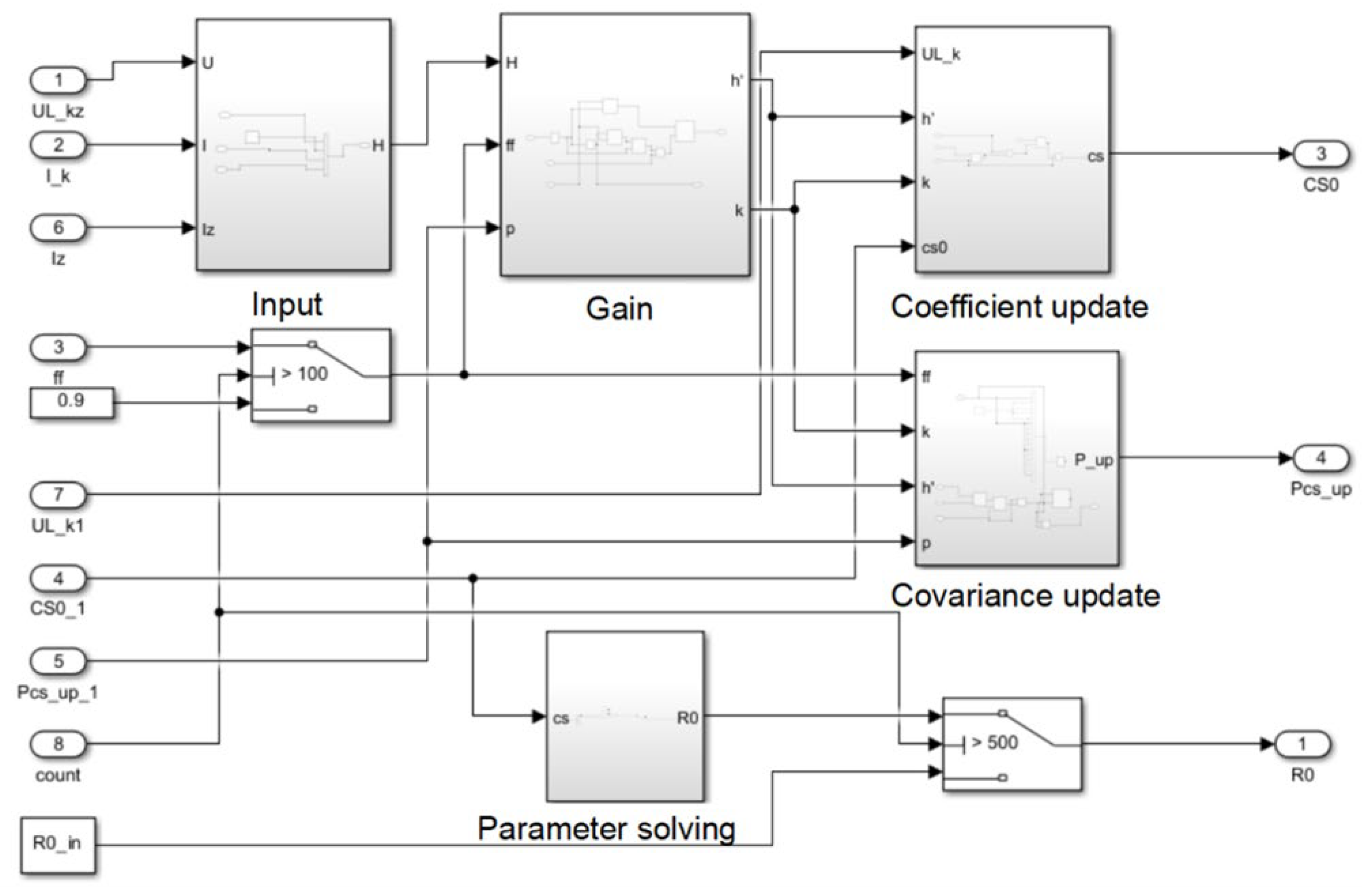
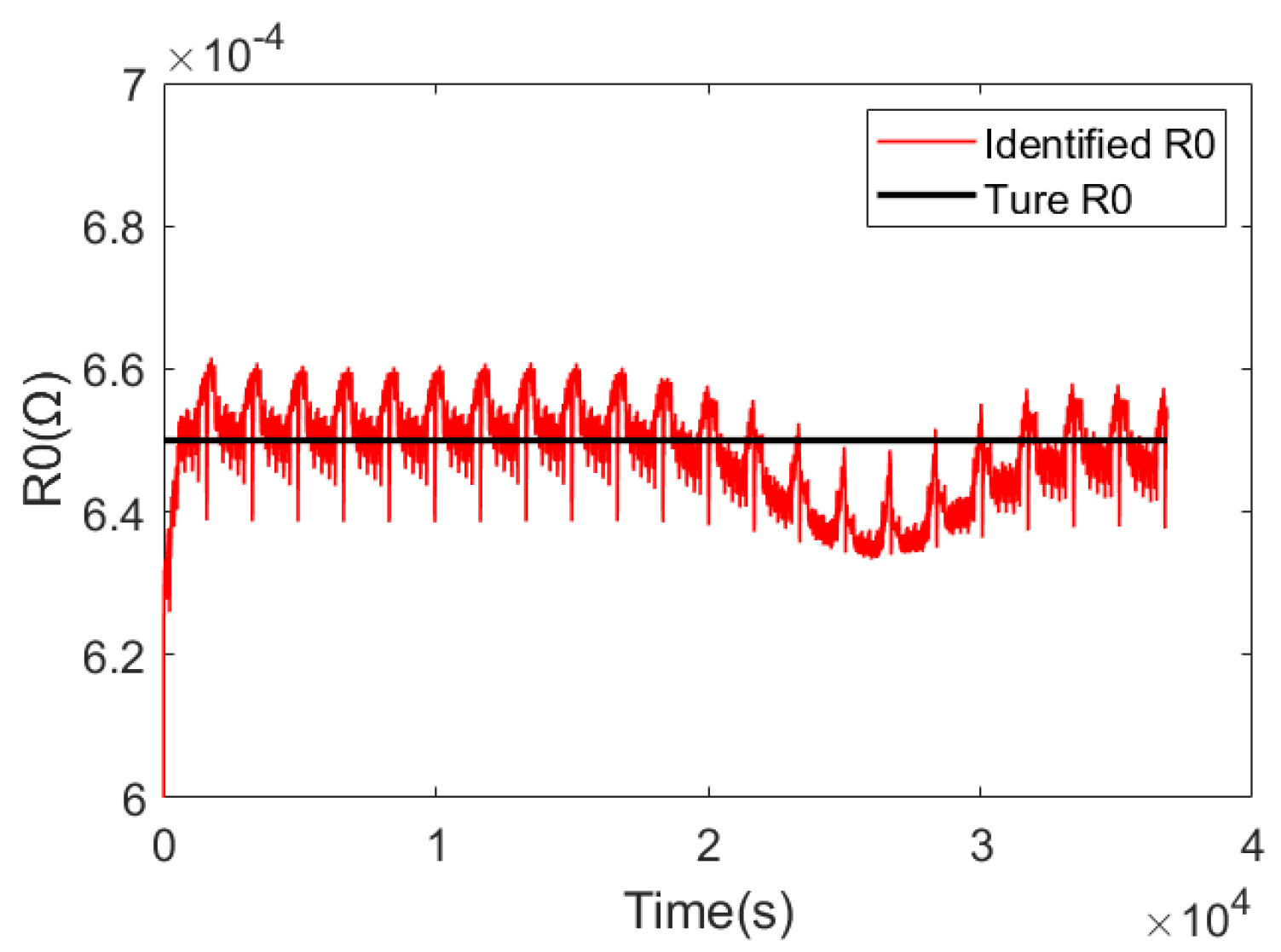
2.3. Online Real-Time Calculation Based on FFRLS Algorithm to Obtain R₀

In this section, R₀ is obtained by an online identification algorithm, and R₀ is updated online on a micro-time scale. R₀ is input into a multi-time-scale SOC and SOH joint estimator for calculation. The R₀ online identification algorithm adopts FFRLS, and the derivation process of its differential equation is consistent with Formulas (5)–(8). The analytical formula can be derived from coefficients α1 and α3, as shown in the following formula.

$${\mathrm{R}}_0=-\frac{{\mathsf{\alpha }}_3}{{\mathsf{\alpha }}_1}$$

(9)

The FFRLS calculation process for R₀ online identification is consistent with Section 2.2. According to the FFRLS pseudo-code table, the R₀ online identification module is established in Simulink. As shown in Figure 5, the identification result when the coefficient is selected as 0.998 is shown in Figure 6. The input of the FFRLS estimation module is the current and voltage at the current moment and the current and voltage from the previous moment, and the output is the estimated value of the ohmic internal resistance R₀. At the same time step, the FFRLS estimation module is the first to be processed, and its results are input into the SOC estimation module for calculation.

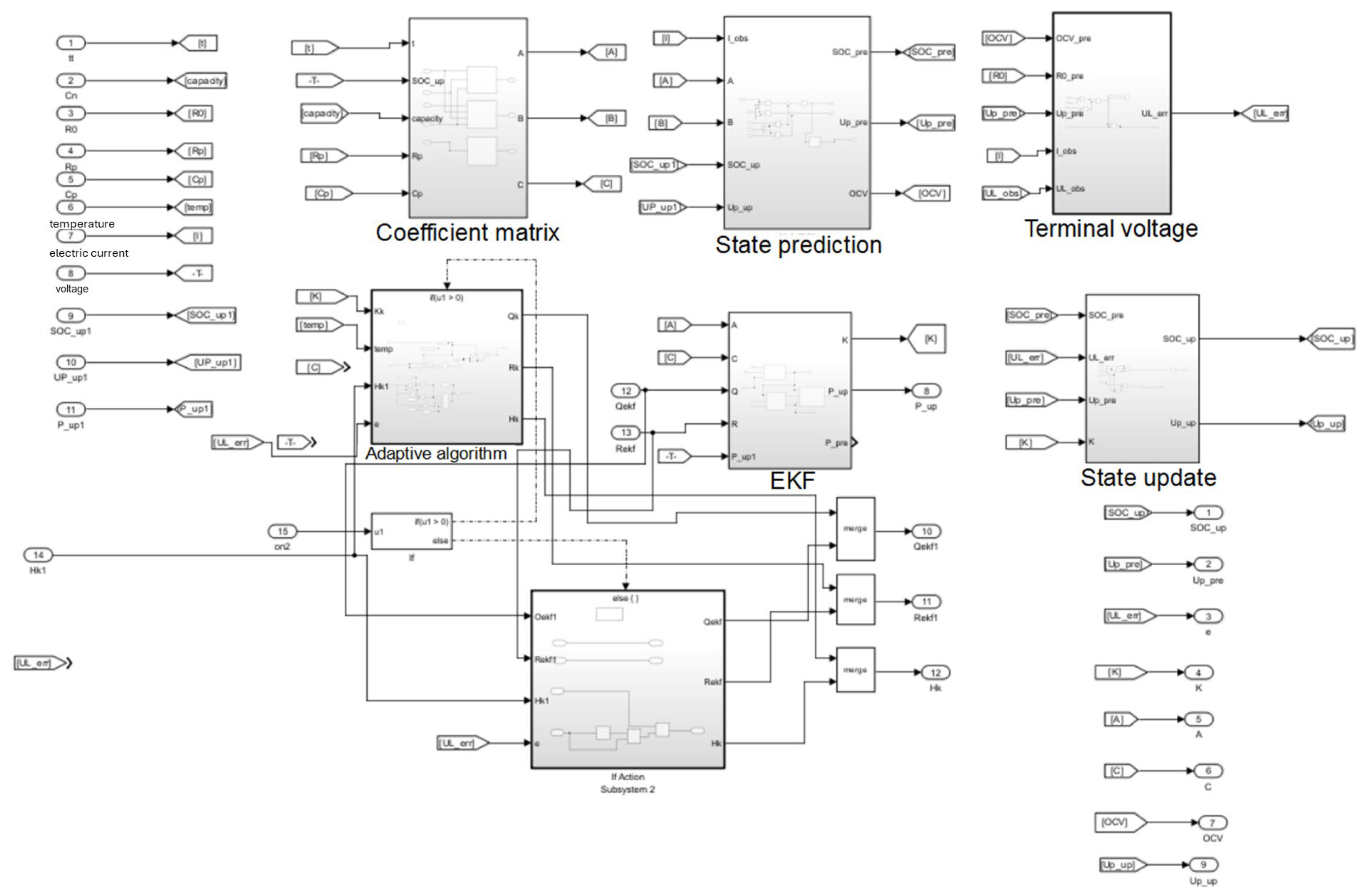
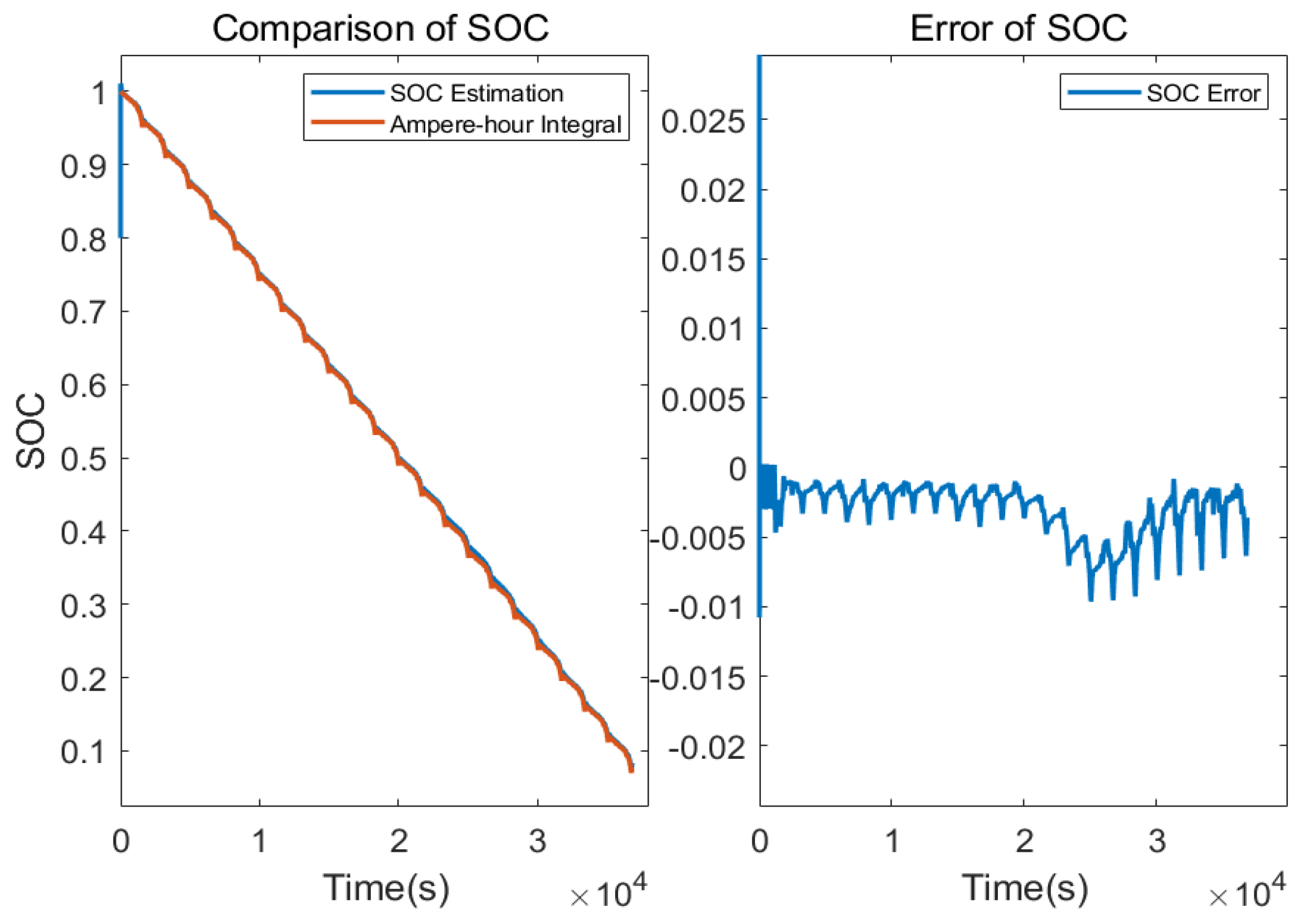
2.4. Micro-Time-Scale SOC Estimation and Simulink Implementation

There is much research on SOC estimation methods, among which EKF is widely used because of its high computational efficiency and estimation accuracy. The AEKF algorithm is improved on the basis of the EKF algorithm and solves the updating problem of process noise and observation noise through an adaptive algorithm, which improves the estimation accuracy and has better adaptability. The AEKF algorithm is used to estimate the micro-time-scale SOC. First, it is necessary to establish the state space equation of the battery system for SOC estimation and linearize the state transition matrix and observation matrix. The state space equation establishment process is shown in the following equation:

$$\left\{\begin{array}{c}{\mathrm{x}}_{\mathrm{k}}=\mathrm{A}{\mathrm{x}}_{\mathrm{k}-1}+\mathrm{B}{\mathrm{u}}_{\mathrm{k}-1}+{\mathsf{\omega }}_{\mathrm{k}-1}\\ {\mathrm{y}}_{\mathrm{k}}=\mathrm{C}{\mathrm{x}}_{\mathrm{k}}+\mathrm{D}{\mathrm{u}}_{\mathrm{k}}+{\mathsf{\upsilon }}_{\mathrm{k}}\end{array}\right.$$

(10)

In the formula, matrix x_k is the state variable of the system at moment k, u_k is the control input variable of the system at moment k, matrix A is the state transition matrix, matrix B is the control input matrix of the system, y_k is the output matrix of the system at moment k, which is the observed signal value of the system, C is the observation matrix, and D is the feedforward matrix. ω_k and υ_k represent process noise and observed noise input to the system, respectively.

Combined with the state space expression of the equivalent circuit model, the state variable is defined as the following formula:

$$\mathrm{x}={\left[{\mathrm{U}}_1\mathrm{S}\mathrm{O}\mathrm{C}\right]}^{\mathrm{T}}$$

(11)

In the equivalent circuit model, the equation of state is linear, while the relationship between OCV-SOC in the observation equation is non-linear, so the observation equation needs to be linearized. The coefficients of the equation of state and the observation equation after linearization are shown in the following equation:

$$\left\{\begin{array}{c}\begin{array}{cc}\mathrm{A}=\left[\begin{array}{cc}{\mathrm{e}}^{-\frac{∆\mathrm{T}}{\mathsf{\tau }}}& 0\\ 0& 1\end{array}\right]& \mathrm{B}=\left[\begin{array}{c}{{\mathrm{R}}_1(1-\mathrm{e}}^{-\frac{∆\mathrm{T}}{\mathsf{\tau }}})\\ \frac{\mathsf{\eta }∆\mathrm{T}}{\mathrm{C}\mathrm{n}}\end{array}\right]\end{array}\\ \begin{array}{cc}\mathrm{C}=\left[\begin{array}{cc}1& \frac{\partial \mathrm{U}\mathrm{o}\mathrm{c}\mathrm{v}}{\partial \mathrm{S}\mathrm{O}\mathrm{C}}\end{array}\right]& \mathrm{D}=\mathrm{R}0\end{array} \end{array}\right.$$

(12)

In the formula, τ represents the time constant, τ = R₁ $\times$ 1.

The state space equation for SOC estimation is now established. Further, the AEKF calculation process is elaborated. Before deducing the algorithm flow, it is necessary to define the micro-time-scale step size and macro-time-scale step size. The micro-time-scale step size is defined as k and k = 1:L, and the macro-time-scale step size is defined as m, and L is the number of micro-time-scale calculation steps included in a macro-time scale. The calculation flow is shown in the following pseudo code (Algorithm 2).

Algorithm 2: Micro-time scale SOC estimation

Input: ${\mathrm{U}}_{\mathrm{t}}\left(\mathrm{k}\right)$$, \mathrm{I}\left(\mathrm{k}\right)$  Output: $\mathrm{S}\mathrm{O}\mathrm{C}$ // Initialize the micro-time-scale SOC estimator ${\mathrm{x}}_0,{\mathrm{P}}_0^{\mathrm{x}},{\mathrm{Q}}_0^{\mathrm{x}},{\mathrm{R}}_0^{\mathrm{x}}$. for k = 1:L // Prior estimate of the state quantities, State error covariance and terminal voltage $${\mathrm{x}}_{\mathrm{m}-1,\mathrm{k}}^{-}={\mathrm{A}}_{\mathrm{m}-1,\mathrm{k}-1}{\mathrm{x}}_{\mathrm{m}-1,\mathrm{k}-1}+{\mathrm{B}}_{\mathrm{m}-1,\mathrm{k}-1}{\mathrm{u}}_{\mathrm{m}-1,\mathrm{k}-1}$$ (13) $${\mathrm{P}}_{\mathrm{m}-1,\mathrm{k}}^{\mathrm{x}-}={{\mathrm{A}}_{\mathrm{m}-1,\mathrm{k}-1}\mathrm{P}}_{\mathrm{m}-1,\mathrm{k}-1}^{\mathrm{x}}{{\mathrm{A}}_{\mathrm{m}-1,\mathrm{k}-1}}^{\mathrm{T}}+{\mathrm{Q}}_{\mathrm{m}-1,\mathrm{k}-1}^{\mathrm{x}}$$ (14) $${\mathrm{y}}_{\mathrm{m}-1,\mathrm{k}}={\mathrm{C}}_{\mathrm{m}-1,\mathrm{k}}{\mathrm{x}}_{\mathrm{m}-1,\mathrm{k}}^{-}+{\mathrm{D}}_{\mathrm{m}-1,\mathrm{k}}{\mathrm{u}}_{\mathrm{m}-1,\mathrm{k}}$$ (15) // Calculate the innovation and Kalman gain $${\mathrm{e}}_{\mathrm{m}-1,\mathrm{k}}={\mathrm{U}}_{\mathrm{m}-1,\mathrm{k}}-{\mathrm{y}}_{\mathrm{m}-1,\mathrm{k}}$$ (16) $${\mathrm{K}}_{\mathrm{m}-1,\mathrm{k}}^{\mathrm{x}}={\mathrm{P}}_{\mathrm{m}-1,\mathrm{k}}^{\mathrm{x}-}{{\mathrm{C}}_{\mathrm{m}-1,\mathrm{k}}}^{\mathrm{T}}{[{\mathrm{C}}_{\mathrm{m}-1,\mathrm{k}}{\mathrm{P}}_{\mathrm{m}-1,\mathrm{k}}^{\mathrm{x}-}{{\mathrm{C}}_{\mathrm{m}-1,\mathrm{k}}}^{\mathrm{T}}+{\mathrm{R}}_{\mathrm{m}-1,\mathrm{k}}^{\mathrm{x}}]}^{-1}$$ (17) // Update status and error coordination error $${\mathrm{x}}_{\mathrm{m}-1,\mathrm{k}}={\mathrm{x}}_{\mathrm{m}-1,\mathrm{k}}^{-}+{\mathrm{K}}_{\mathrm{m}-1,\mathrm{k}}^{\mathrm{x}}{\mathrm{e}}_{\mathrm{m}-1,\mathrm{k}}$$ (18) $${\mathrm{P}}_{\mathrm{m}-1,\mathrm{k}}^{\mathrm{x}}=[{\mathrm{I}}^{\mathrm{’}}-{\mathrm{K}}_{\mathrm{m}-1,\mathrm{k}}^{\mathrm{x}}{\mathrm{C}}_{\mathrm{m}-1,\mathrm{k}}]{\mathrm{P}}_{\mathrm{m}-1,\mathrm{k}}^{\mathrm{x}-}$$ (19) // Adaptive update Qx and Rx $${\mathrm{H}}_{\mathrm{m}-1,\mathrm{k}}=\frac{1}{\mathrm{M}\_\mathrm{m}\mathrm{i}\mathrm{c}}{\sum }_{\mathrm{i}=\mathrm{k}-\mathrm{M}\_\mathrm{m}\mathrm{i}\mathrm{c}}^{\mathrm{k}}{\mathrm{e}}_{\mathrm{m}-1,\mathrm{k}}{\mathrm{e}}_{\mathrm{m}-1,\mathrm{k}}^{\mathrm{T}}$$ (20) $${\mathrm{Q}}_{\mathrm{m}-1,\mathrm{k}}^{\mathrm{x}}={\mathrm{K}}_{\mathrm{m}-1,\mathrm{k}}^{\mathrm{x}}{\mathrm{H}}_{\mathrm{m}-1,\mathrm{k}}{{\mathrm{K}}_{\mathrm{m}-1,\mathrm{k}}^{\mathrm{x}}}^{\mathrm{T}}$$ (21) $${\mathrm{R}}_{\mathrm{m}-1,\mathrm{k}}^{\mathrm{x}}={\mathrm{H}}_{\mathrm{m}-1,\mathrm{k}}+{\mathrm{C}}_{\mathrm{m}-1,\mathrm{k}}{\mathrm{P}}_{\mathrm{m}-1,\mathrm{k}}^{\mathrm{x}}{{\mathrm{C}}_{\mathrm{m}-1,\mathrm{k}}}^{\mathrm{T}}$$ (22) // The micro-time-scale k = L $$\left\{\begin{array}{c}{\mathrm{x}}_{\mathrm{m},0}={\mathrm{x}}_{\mathrm{m}-1,\mathrm{L}}\\ {\mathrm{P}}_{\mathrm{m},0}^{\mathrm{x}}={\mathrm{P}}_{\mathrm{m}-1,\mathrm{L}}^{\mathrm{x}}\\ {\mathrm{e}}_{\mathrm{m},0}={\mathrm{e}}_{\mathrm{m}-1,\mathrm{L}}\\ {\mathrm{u}}_{\mathrm{m},0}={\mathrm{u}}_{\mathrm{m}-1,\mathrm{L}}\end{array}\right.$$ (23) end

According to the pseudo-code table of the AEKF algorithm, the SOC estimation module is established in Simulink, as shown in Figure 7. The SOC estimation results are shown in Figure 8.

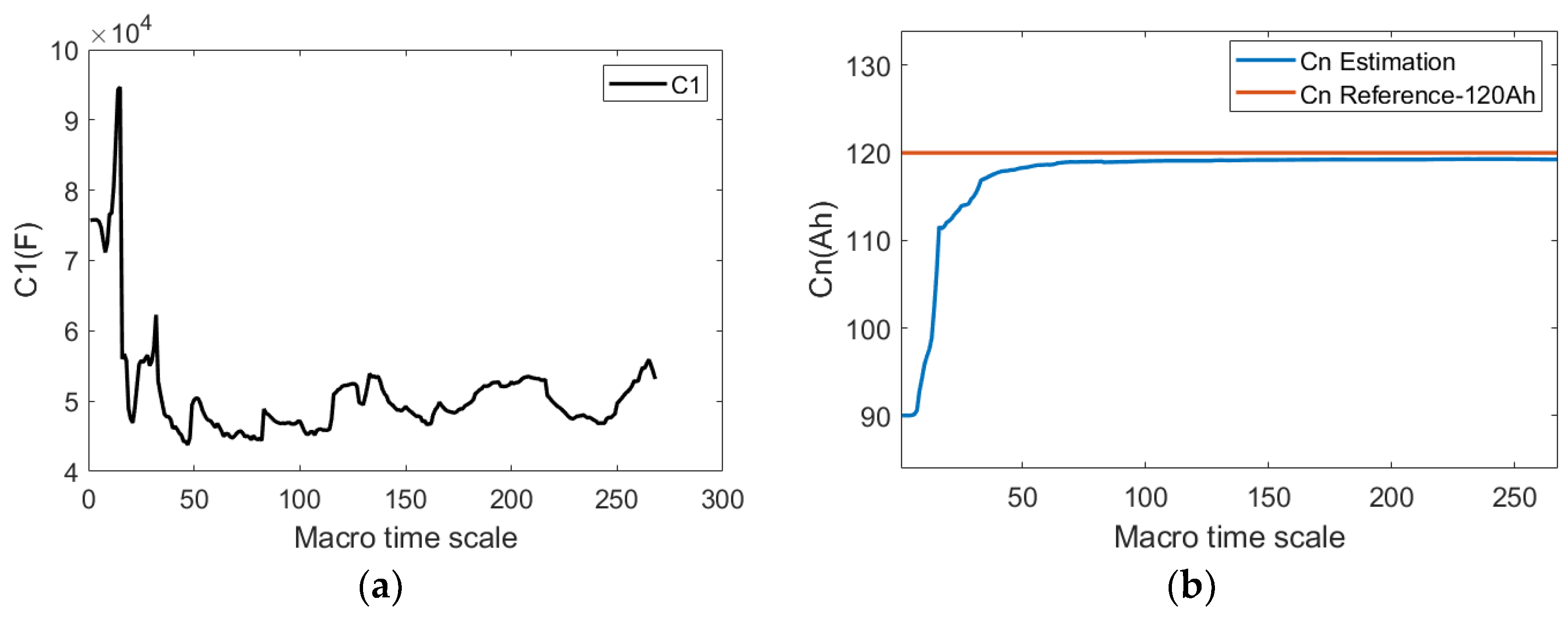
2.5. Macro-Time-Scale C₁ and C_n Estimation and Simulink Implementation

The macro-time-scale C₁ and capacity estimation schemes are implemented by the AEKF algorithm. Although the battery parameter R₁ is a fixed value, it is close to the real value of R₁, but there are still some errors. Therefore, the polarization voltage error caused by the R₁ error is corrected by the online estimation of C₁ to improve the estimation accuracy of the polarization voltage. Before the macro-time-scale estimator is turned on, it is necessary to ensure that the error of the initial value of the battery state is as small as possible, so as to avoid the output of large innovation during the callback of the micro-time-scale SOC estimator, which makes the macro-time-scale estimator fluctuate violently or even diverge. Therefore, the first 200-step macro-time-scale estimator does not work when the computation begins, and the multi-time-scale double Kalman filter degenerates into a single Kalman filter. When the length of the calculation is 200 steps, the macro-time-scale estimator will boot and begin the joint estimation of SOC and SOH. The macro-time-scale estimator updates C₁ and capacity values through the calculation results of the first 200 steps and inputs the micro-time scale for SOC calculation. When the calculation of the micro-time scale reaches the judgment condition of the next macro-time scale, the macro-time-scale estimator jumps out and updates the polarization parameter and capacity value through the calculation results of the previous macro-time scale. Iterate through this step until the calculation is complete. The calculation process of the macro-time-scale estimator is as follows:

Firstly, the state-space equation for the macro-time-scale parameter estimator is established, as shown in Equation (24):

$$\left\{\begin{array}{c}{\mathsf{\varphi }}_{\mathrm{k}}={\mathsf{\varphi }}_{\mathrm{k}-1}+{\mathsf{\omega }}_{\mathrm{k}-1}^{\mathsf{\varphi }}\\ {\mathrm{y}}_{\mathrm{k}}=\mathrm{C}{\mathrm{x}}_{\mathrm{k}}+\mathrm{D}{\mathrm{u}}_{\mathrm{k}}+{\mathsf{\upsilon }}_{\mathrm{k}}\end{array}\right.$$

(24)

In equation $\mathsf{\varphi }={({\mathrm{C}}_1,{\mathrm{C}}_{\mathrm{n}})}^{\mathrm{T}}$, the observation matrix is consistent with Equation (12), which is the terminal voltage calculation formula.

Then the iterative process of the Kalman filter is calculated, and the algorithm flow is shown in the following pseudo code (Algorithm 3).

Algorithm 3: Macro-time-scale C1 and Cn estimation

Input: ${\mathrm{U}}_{\mathrm{t}}\left(\mathrm{k}\right)$$, \mathrm{I}\left(\mathrm{k}\right)$ Output: ${\mathrm{C}}_1,{\mathrm{C}}_{\mathrm{n}}$ // Initialize the macro-time-scale parameter estimator ${\mathsf{\varphi }}_0,{\mathrm{P}}_0^{\mathsf{\varphi }},{\mathrm{Q}}_0^{\mathsf{\varphi }},{\mathrm{R}}_0^{\mathsf{\varphi }}$. // The calculation of parameters and parameter error covariance prior estimates. $${\mathsf{\varphi }}_{\mathrm{m}}^{-}={\mathsf{\varphi }}_{\mathrm{m}-1}$$ (25) $${\mathrm{P}}_{\mathrm{m}}^{\mathsf{\varphi }-}={\mathrm{P}}_{\mathrm{m}-1}^{\mathsf{\varphi }}+{\mathrm{Q}}_{\mathrm{m}-1}^{\mathsf{\varphi }}$$ (26) // The equation of state and observations. $${\mathrm{x}}_{\mathrm{k}}=\mathrm{A}{\mathrm{x}}_{\mathrm{k}-1}+\mathrm{B}{\mathrm{u}}_{\mathrm{k}-1}+{\mathsf{\omega }}_{\mathrm{k}-1}=\mathrm{F}({\mathrm{x}}_{\mathrm{k}},{\mathrm{u}}_{\mathrm{k}},\mathsf{\varphi })$$ (27) $${\mathrm{y}}_{\mathrm{k}}=\mathrm{C}{\mathrm{x}}_{\mathrm{k}}+\mathrm{D}{\mathrm{u}}_{\mathrm{k}}+{\mathsf{\upsilon }}_{\mathrm{k}}=\mathrm{G}({\mathrm{x}}_{\mathrm{k}},{\mathrm{u}}_{\mathrm{k}},\mathsf{\varphi })$$ (28) // Parameter estimator Kalman gain update. $$\left\{\begin{array}{c}{\mathrm{C}}_{\mathrm{m}}^{\mathsf{\varphi }}=\frac{\mathrm{d}\mathrm{G}({\mathrm{x}}_{\mathrm{m},0},{\mathrm{u}}_{\mathrm{m},0},{\mathsf{\varphi }}_{\mathrm{m}}^{-})}{\mathrm{d}\mathsf{\varphi }}=\frac{\partial \mathrm{G}({\mathrm{x}}_{\mathrm{m},0},{\mathrm{u}}_{\mathrm{m},0},{\mathsf{\varphi }}_{\mathrm{m}}^{-})}{\partial {\mathsf{\varphi }}_{\mathrm{m}}^{-}}+\frac{\partial \mathrm{G}({\mathrm{x}}_{\mathrm{m},0},{\mathrm{u}}_{\mathrm{m},0},{\mathsf{\varphi }}_{\mathrm{m}}^{-})}{\partial {\mathrm{x}}_{\mathrm{m},0}}\frac{\mathrm{d}{\mathrm{x}}_{\mathrm{m},0}}{\mathrm{d}{\mathsf{\varphi }}_{\mathrm{m}}^{-}}\\ \frac{\mathrm{d}{\mathrm{x}}_{\mathrm{m},0}}{\mathrm{d}{\mathsf{\varphi }}_{\mathrm{m}}^{-}}=\frac{\partial \mathrm{F}({\widehat{\mathrm{x}}}_{\mathrm{m}-1,\mathrm{L}-1},{\mathrm{u}}_{\mathrm{m}-1,\mathrm{L}-1},{\mathsf{\varphi }}_{\mathrm{m}}^{-})}{\partial {\mathsf{\varphi }}_{\mathrm{m}}^{-}}+\frac{\partial \mathrm{F}({\widehat{\mathrm{x}}}_{\mathrm{m}-1,\mathrm{L}-1},{\mathrm{u}}_{\mathrm{m}-1,\mathrm{L}-1},{\mathsf{\varphi }}_{\mathrm{m}}^{-})}{\partial {\widehat{\mathrm{x}}}_{\mathrm{m}-1,\mathrm{L}-1}}\frac{\mathrm{d}{\widehat{\mathrm{x}}}_{\mathrm{m}-1,\mathrm{L}-1}}{\mathrm{d}{\mathsf{\varphi }}_{\mathrm{m}}^{-}}\\ \frac{\mathrm{d}{\widehat{\mathrm{x}}}_{\mathrm{m}-1,\mathrm{L}-1}}{\mathrm{d}{\mathsf{\varphi }}_{\mathrm{m}}^{-}}=\frac{\partial \mathrm{F}({\mathrm{x}}_{\mathrm{m}-1,\mathrm{L}-1},{\mathrm{u}}_{\mathrm{m}-1,\mathrm{L}-1},{\mathsf{\varphi }}_{\mathrm{m}}^{-})}{\partial {\mathsf{\varphi }}_{\mathrm{m}}^{-}}+{\mathrm{K}}_{\mathrm{m}-1,\mathrm{L}-1}^{\mathrm{x}}\frac{\mathrm{d}\mathrm{G}({\mathrm{x}}_{\mathrm{m}-\mathrm{1,0}},{\mathrm{u}}_{\mathrm{m}-\mathrm{1,0}},{\mathsf{\varphi }}_{\mathrm{m}-1}^{-})}{\mathrm{d}\mathsf{\varphi }}\end{array}\right.$$ (29) $${\mathrm{K}}_{\mathrm{m}}^{\mathsf{\varphi }}={\mathrm{P}}_{\mathrm{m}}^{\mathsf{\varphi }-}{{\mathrm{C}}_{\mathrm{m}}^{\mathsf{\varphi }}}^{\mathrm{T}}{[{\mathrm{C}}_{\mathrm{m}}^{\mathsf{\varphi }}{\mathrm{P}}_{\mathrm{m}}^{\mathsf{\varphi }-}{{\mathrm{C}}_{\mathrm{m}}^{\mathsf{\varphi }}}^{\mathrm{T}}+{\mathrm{R}}_{\mathrm{m}}^{\mathsf{\varphi }}]}^{-1}$$ (30) // The state update of the parameter estimator and error covariance. $${\mathrm{Q}}_{\mathrm{m}-1,\mathsf{k}}^{\mathsf{\varphi }}={\mathsf{K}}_{\mathrm{m}-1,\mathsf{k}}^{\mathsf{\varphi }}{\mathrm{H}}_{\mathrm{m}-1,\mathsf{k}}^{\mathsf{\varphi }}{{\mathsf{K}}_{\mathrm{m}-1,\mathsf{k}}^{\mathsf{\varphi }}}^{\mathrm{T}}$$ (31) $${\mathrm{R}}_{\mathrm{m}-1,\mathsf{k}}^{\mathsf{\varphi }}={\mathrm{H}}_{\mathrm{m}-1,\mathsf{k}}^{\mathsf{\varphi }}+{{\mathrm{C}}_{\mathrm{m}-1,\mathsf{k}}^{\mathsf{\varphi }}\mathrm{P}}_{\mathrm{m}-1,\mathsf{k}}^{\mathsf{\varphi }}{{\mathrm{C}}_{\mathrm{m}-1,\mathsf{k}}^{\mathsf{\varphi }}}^{\mathrm{T}}$$ (32) // Adaptive update ${\mathrm{Q}}^{\mathsf{\Phi }} \mathrm{a}\mathrm{n}\mathrm{d} {\mathrm{R}.}^{\mathsf{\Phi }}$ $${\mathrm{H}}_{\mathrm{m}-1,\mathrm{k}}^{\mathsf{\varphi }}=\frac{1}{\mathrm{M}\_\mathrm{m}\mathrm{a}\mathrm{c}}{\sum }_{\mathrm{i}=\mathrm{k}-\mathrm{M}\_\mathrm{m}\mathrm{a}\mathrm{c}}^{\mathrm{k}}{\mathrm{e}}_{\mathrm{m}-1,\mathrm{k}}{\mathrm{e}}_{\mathrm{m}-1,\mathrm{k}}^{\mathrm{T}}$$ (33) $${\mathrm{Q}}_{\mathrm{m}-1,\mathsf{k}}^{\mathsf{\varphi }}={\mathsf{K}}_{\mathrm{m}-1,\mathsf{k}}^{\mathsf{\varphi }}{\mathrm{H}}_{\mathrm{m}-1,\mathsf{k}}^{\mathsf{\varphi }}{{\mathsf{K}}_{\mathrm{m}-1,\mathsf{k}}^{\mathsf{\varphi }}}^{\mathrm{T}}$$ (34) $${\mathrm{R}}_{\mathrm{m}-1,\mathsf{k}}^{\mathsf{\varphi }}={\mathrm{H}}_{\mathrm{m}-1,\mathsf{k}}^{\mathsf{\varphi }}+{{\mathrm{C}}_{\mathrm{m}-1,\mathsf{k}}^{\mathsf{\varphi }}\mathrm{P}}_{\mathrm{m}-1,\mathsf{k}}^{\mathsf{\varphi }}{{\mathrm{C}}_{\mathrm{m}-1,\mathsf{k}}^{\mathsf{\varphi }}}^{\mathrm{T}}$$ (35) end

According to the pseudo-code table of C₁ and C_n estimation, C₁ and C_n estimation modules were established in Simulink, as shown in Figure 9.

The estimation of macro-time-scale C₁ and capacity can be realized through continuous iterative calculation through the iterative process of the Kalman filter. The final capacity estimation result is taken as the mean value of 40% of the capacity value calculated on the macroscopic time scale, as shown in Equation (36). Further, the battery SOH was calculated by Formula (2).

$${\mathrm{C}}_{\mathrm{n}}=\mathrm{m}\mathrm{e}\mathrm{a}\mathrm{n}\left({\mathrm{C}}_{\mathrm{n}}\right(0.6\times \mathrm{N}:\mathrm{N}\left)\right)$$

(36)

In the formula, N is the total length of the capacity calculation results on a macro-time scale.

Considering that the initial value of the battery capacity is different at different temperatures, if the same initial value is used, the SOH estimation results will be different at different temperatures. In order to ensure the stability of the SOH estimation results, the temperature-capacity functional relationship is established according to the capacity value of the battery:

$${\mathrm{C}}_{\mathrm{n}\_\mathrm{i}\mathrm{n}\mathrm{i}}={\mathsf{\beta }}_1\times \mathrm{T}+\frac{{\mathrm{C}}_{\mathrm{n}\_\mathrm{i}\mathrm{n}\mathrm{i}}}{3600}-{\mathsf{\beta }}_2$$

(37)

In the formula, T is the battery temperature; ${\mathsf{\beta }}_1=0.48;{\mathsf{\beta }}_2=12$.

The estimated results of C₁ and C_n are shown in Figure 10.

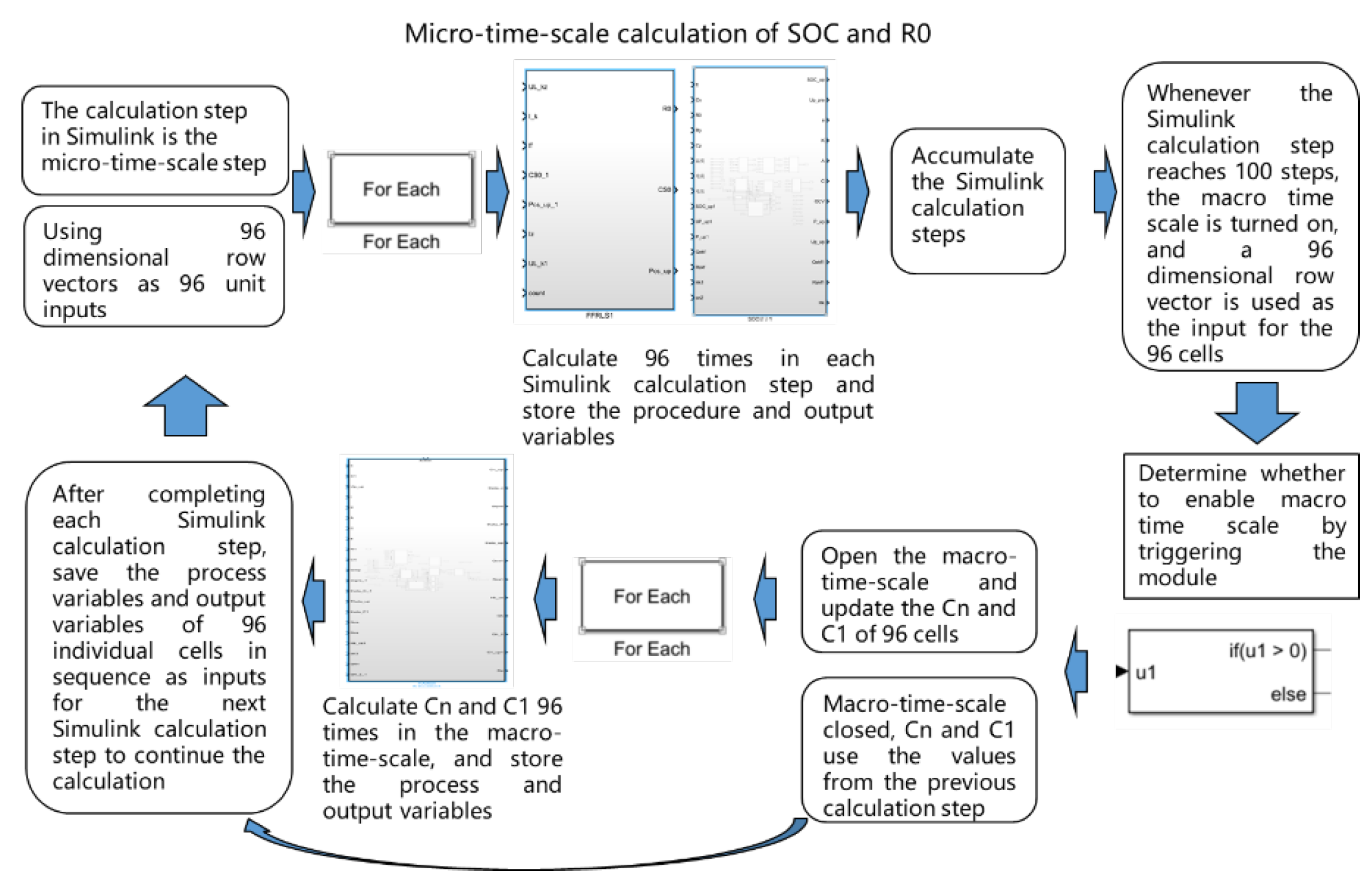
2.6. Sequential Cycle Calculation of 96 Series Connected Cells of Simulink Implementation

The Simulink model for joint estimation of SOC and SOH in 96 batteries consists of three parts: Input, output, and sequential cycle calculation. The inputs are: Current, voltage, and sampling interval; the output is: SOC, capacity, and model parameters for online identification; the sequential cycle calculation module is constructed by the For Each module, and the voltage input for each calculation step is composed of a 1 × 96 matrix, representing 1–96 battery voltages. The For Each module sequentially calls the voltage input joint estimation model for calculation [16], and the process variables in the calculation are stored sequentially for the next calculation step.

At the micro-time scale, for each step of calculation, a matrix form with an input of 1 × 96 is sequentially called, and the For Each module sequentially calls the input to complete 96 calculations of the joint estimation algorithm. After that, the process variables and output variables are stored in a matrix form of 1 × 96 for the next Simulink calculation step. After the macro-time scale is enabled, the For Each module sequentially calls the macro-time-scale estimation algorithm 96 times to update the macro-time-scale parameters and process variables. After the current Simulink calculation step is completed, the macro-time scale is closed, and the updated parameter variables are input into the micro-time scale for calculation until the next macro-time-scale is opened. The 96-cell joint estimation algorithm based on the For Each module implemented by Simulink is shown in Figure 11.

3. HIL Experimental Testing and Result Analysis

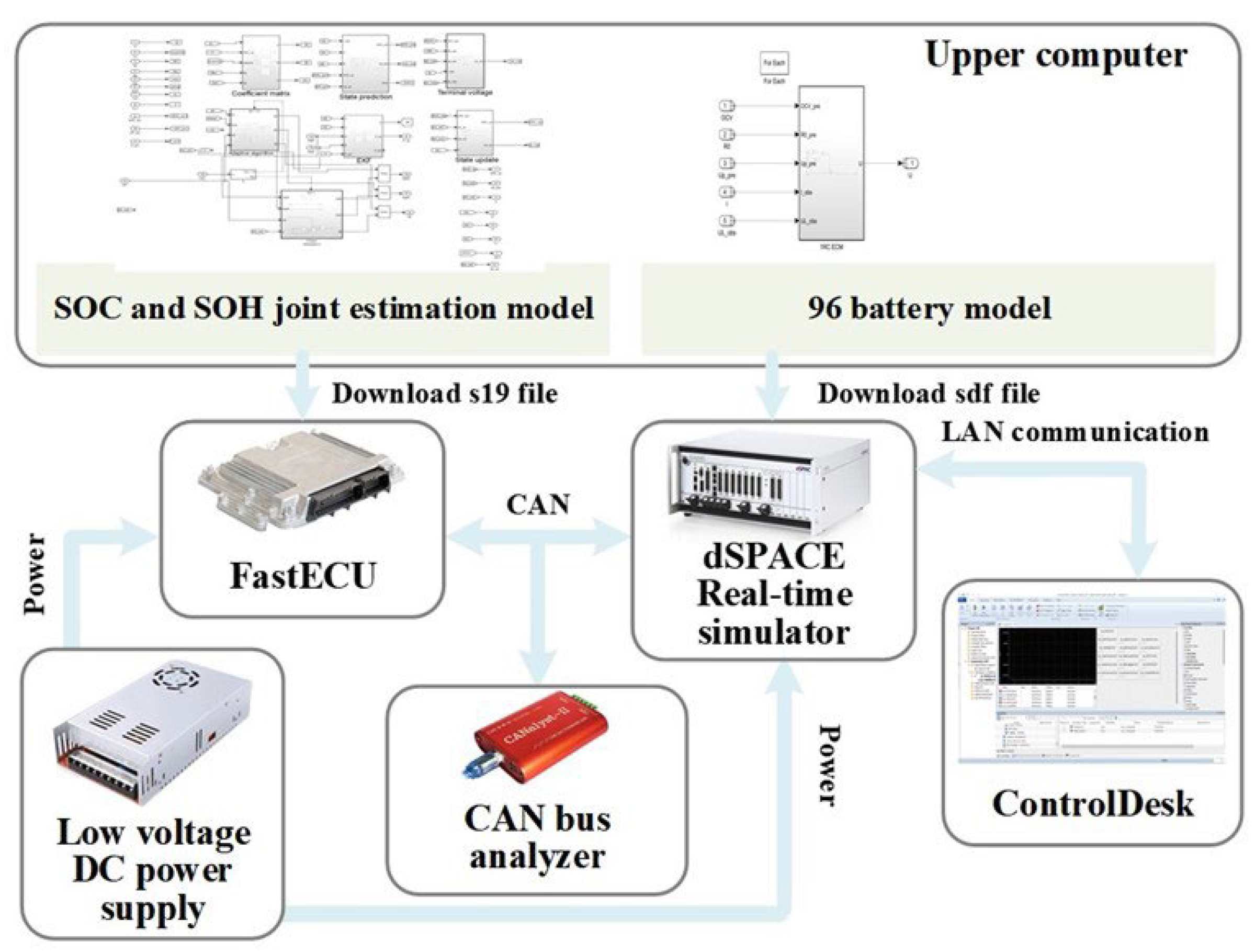
3.1. Introduction to Hardware Implementation Scheme of HIL

According to the V-shaped development process of the electronic control system, after verifying the control effect of the system through offline simulation, it is also necessary to verify the real-time performance and control robustness of the proposed control strategy through experiments [17]. In order to verify the real-time performance of the joint estimation algorithm for SOC and SOH in 96 cells, this paper designs a HIL test plan for the joint estimation algorithm of SOC and SOH, as shown in Figure 12, which mainly includes a PC upper computer, ControlDesk control platform, FastECU rapid prototype controller, dSPACE real-time simulator, CAN bus analyzer, and low-voltage DC power supply.

In the joint estimation algorithm and cell signal generation module established using Simulink mentioned above, the MATLAB/Simulink model built is first divided into two parts in the PC upper computer: The cell signal generation module and the state joint estimation algorithm model. Secondly, compile the joint estimation algorithm model into an s19 file in the ERT environment and flash it into the FastECU rapid prototype controller. Then, compile the battery simulation model into an SDF file in the RTI environment and load it into the dSPACE real-time simulation simulator. Finally, the real-time status of cell voltage and current is calculated and updated in dSPACE, which is then transmitted to FastECU to perform state estimation. The status calculated by FastECU will be sent to the CAN bus for dSPACE to receive and analyze the evaluation results. The above information exchange process is repeated for real-time simulation to achieve HIL testing of the joint estimation algorithm. Among them, the information exchange between the dSPACE real-time simulation simulator and the FastECU rapid prototype controller is achieved through the CAN communication network, with a communication baud rate set to 250 kbps. At the same time, a DBC database file is written and imported to achieve a mapping relationship between the battery cell status and estimation results and the CAN message signal. And create a visual interface in the ControlDesk control platform to monitor and record key variables such as cell voltage and estimation results during the testing process in real time. Unlike the use of bias models to simulate multiple cells in [17], this paper simulates the cell cycle by utilizing the For Each module’s cyclic call to calculate, simulate, and transmit the voltage of the cell under current excitation.

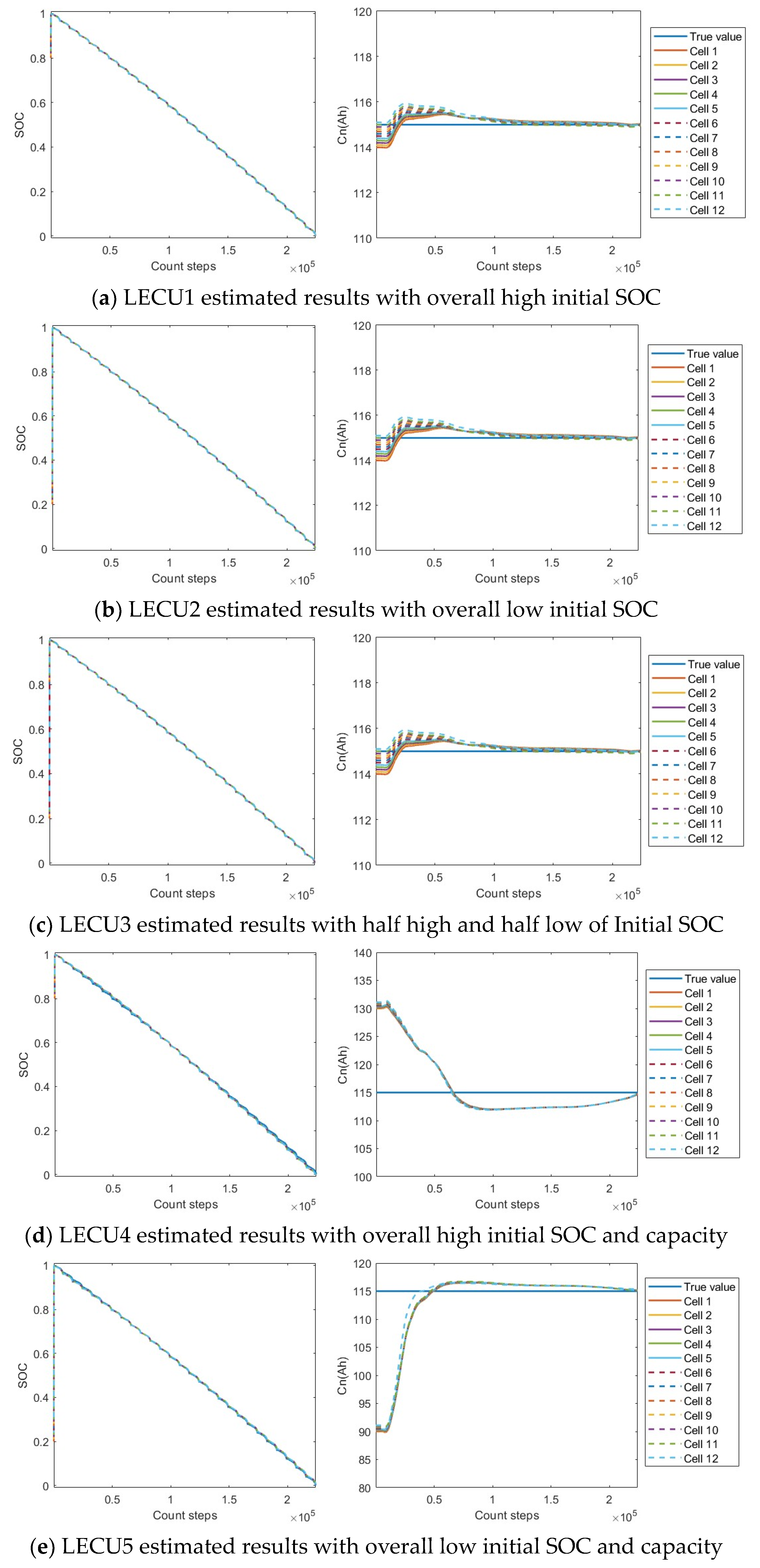
3.2. Multi-Scenarios Testing Scheme

In order to verify the real-time and effective processing of the controller used for joint estimation of 96 cells, as well as the high-precision performance of the algorithm written, a multi-scenario-estimation result verification scheme was designed as shown in

Table 1. Validation of multi-scenarios estimation results.

Initial Deviations/Corresponding LECU and Subfigures of Figure 13			Verification Purposes
Overall high initial SOC/LECU1-Figure 13a	Overall low initial SOC/LECU2-Figure 13b	Initial SOC half high and half low /LECU3-Figure 13c	Deviation cell and amplitude do not affect the accuracy of SOC estimation
Overall high initial SOC and high initial capacity/LECU4-Figure 13d	Overall low initial SOC and low initial capacity/LECU5-Figure 13e	Initial SOC and capacity are both half high and half low/LECU6-Figure 13f	The combination deviation of initial SOC and capacity does not affect the accuracy of SOC estimation and capacity regression
High initial SOC and high model parameters/LECU7-Figure 13g	Low initial SOC and low model parameters/LECU8-Figure 13h	/	The combination deviation of initial SOC and model parameters does not affect the accuracy of SOC estimation and capacity regression

. The estimated results of 96 cells corresponded to 8 LECUs based on the actual electrical architecture of the BMS, where each LECU was responsible for the voltage collection of 12 battery cells [18]. Based on the flexibility of HIL testing and verification purposes, initial value deviations were set for each LECU. The estimated results are shown in Figure 13.

3.3. Real Time Estimation Result Analysis

Figure 13 shows the calculation results of 96 cells at both micro- and macro-time scales. Subfigures (a) to (h) correspond to the 8 initial deviation verification schemes shown in Table 1, respectively.

From the results of Figure 13a–c, it can be seen that when the initial SOC values of cells in LECU1, LECU2, and LECU3 are set to the range of 0.8–0.9 and 0.2–0.3, respectively, and the initial capacity value is set to the vicinity of the true value, the algorithm can quickly correct the SOC value to the vicinity of the true value, and the estimated results of 12 batteries are close to the true value, with high accuracy. The estimation results of capacity have a small range of fluctuations in the early stage, which is related to the inaccurate initial values of SOC in the early stage and the adaptive adjustment process of process noise and observation noise in the macro-time-scale estimator. As the error between the fluctuation range of capacity and the true value is less than 1%, this article believes that the capacity estimation results have high accuracy. The above results indicate that the initial error of the proposed algorithm’s SOC has a relatively small impact on the joint estimation of SOC and capacity, and the deviation position and amplitude do not affect the accuracy of SOC estimation and show the same regression time for capacity calculation.

From the results of Figure 13d–f, it can be seen that when the initial SOC value of the battery in LECU4 is in the high SOC range and the initial capacity value is greater than the true capacity value, the initial SOC value of the battery in LECU5 is in the low SOC range and the initial capacity value is less than the true capacity value, half of the initial SOC value of the battery in LECU6 is in the low SOC range and half is in the high SOC range, and half of the initial capacity value is less than the true capacity value and half is greater than the true capacity value, the algorithm can correct the SOC and capacity values of the batteries in the three sets of LECUs to near the true value. The SOC estimation error is less than 2%, and the capacity estimation error is less than 3%. The results indicate that the estimation accuracy and stability of the proposed algorithm are less affected by the initial values of SOC and capacity.

From the results of Figure 13g,h, it can be seen that when the initial value of battery SOC in LECU7 is in the high SOC range and the initial value of battery parameters is higher than the true value, and the initial value of battery SOC in LECU8 is in the low SOC range and the initial value of battery parameters is lower than the true value, the proposed algorithm can quickly correct SOC to near the true value, thereby ensuring high SOC estimation accuracy and capacity estimation accuracy.

In summary, the proposed algorithm and its solution method can not only achieve synchronous calculation of 96 cells but also have high estimation accuracy and stability under various bias combination input conditions.

4. Conclusions

To verify the real-time performance and accuracy of the joint estimation algorithm for high-voltage battery packs composed of 96 individual cells in series, On the basis of writing the state equations of 1RC discretized equivalent circuits and deriving them using FFRLS and DAEKF algorithms, this article applies Simulink to develop a joint estimation algorithm for SOC and SOH based on the 1RC ECM and implements the algorithm’s cyclic calling for series nodes, enhancing the algorithm’s scalability. In the algorithm, the FFRLS is applied to calculate OCV, R₀, and R₁ in the time domain, and the DAEKF is applied to the joint estimation of SOC and SOH at multiple time scales. After gradually verifying the Simulink algorithm model, with the help of dSPACE and FASECU controllers, HIL testing was completed in multiple scenarios. The results showed that the proposed algorithm and its solution method can not only achieve synchronous calculation of 96 cells but also have high estimation accuracy and stability under various bias combination input conditions, laying the foundation for future applications of electric vehicles.

References

1. Khan, F.N.U.; Rasul, M.G.; Sayem, A.S.M.; Mandal, N.K. Design and optimization of lithium-ion battery as an efficient energy storage device for electric vehicles: A comprehensive review. J. Energy Storage 2023, 71, 108033. [Google Scholar] [CrossRef]
2. Chen, Y.; Li, R.; Sun, Z.; Zhao, L.; Guo, X. SOC estimation of retired lithium-ion batteries for electric vehicle with improved particle filter by H-infinity filter. Energy Rep. 2023, 9, 1937–1947. [Google Scholar] [CrossRef]
3. Li, X.; Wang, Z.; Zhang, L. Co-estimation of capacity and state-of-charge for lithium-ion batteries in electric vehicles. Energy 2019, 174, 33–44. [Google Scholar] [CrossRef]
4. Shen, P.; Ouyang, M.; Lu, L.; Li, J.; Feng, X. The Co-Estimation of State of Charge, State of Health, and State of Function for Lithium-ion Batteries in Electric Vehicles. IEEE Trans. Veh. Technol. 2017, 67, 92–103. [Google Scholar] [CrossRef]
5. Guo, F.; Hu, G.; Xiang, S.; Zhou, P.; Hong, R.; Xiong, N. A multi-scale parameter adaptive method for state of charge and parameter estimation of lithium-ion batteries using dual Kalman filters. Energy 2019, 178, 79–88. [Google Scholar] [CrossRef]
6. Shuzhi, Z.; Xu, G.; Xiongwen, Z. A novel one-way transmitted co-estimation framework for capacity and state-of-charge of lithium-ion battery based on double adaptive extended Kalman filters. J. Energy Storage 2021, 33, 102093. [Google Scholar] [CrossRef]
7. Arora, S.; Shen, W.; Kapoor, A. Critical analysis of open circuit voltage and its effect on estimation of irreversible heat for Li-ion pouch cells. J. Power Sources 2017, 350, 117–126. [Google Scholar] [CrossRef]
8. Yun, X.; Zhang, X.; Wang, C.; Fan, X. Online parameters identification and state of charge estimation for lithium-ion batteries based on improved central difference particle filter. J. Energy Storage 2023, 70, 107987. [Google Scholar] [CrossRef]
9. Zheng, Y.; Cui, Y.; Han, X.; Dai, H.; Ouyang, M. Lithium-ion battery capacity estimation based on open circuit voltage identification using the iteratively reweighted least squares at different aging levels. J. Energy Storage 2021, 44, 103487. [Google Scholar] [CrossRef]
10. Dai, H.; Xu, T.; Zhu, L.; Wei, X.; Sun, Z. Adaptive model parameter identification for large capacity Li-ion batteries on separated time scales. Appl. Energy 2016, 184, 119–131. [Google Scholar] [CrossRef]
11. Plett, G.L. Efficient battery pack state estimation using Bar-delta filtering. In Proceedings of the EVS24 International Battery, Hybrid and Fuel Cell Electric Vehicle Symposium, Stavanger, Norway, 13–16 May 2009. [Google Scholar]
12. Dai, H.; Wei, X.; Sun, Z.; Wang, J.; Gu, W. Online cell SOC estimation of Li-ion battery packs using a dual time-scale Kalman filtering for EV applications. Appl. Energy 2012, 95, 227–237. [Google Scholar] [CrossRef]
13. Jiang, B.; Dai, H.; Wei, X. A Cell-to-Pack State Estimation Extension Method Based on a Multilayer Difference Model for Series-Connected Battery Packs. IEEE Trans. Transp. Electrif. 2021, 8, 2037–2049. [Google Scholar] [CrossRef]
14. Pai, H.Y.; Liu, Y.H.; Ye, S.P. Online estimation of lithium-ion battery equivalent circuit model parameters and state of charge using time-domain assisted decoupled recursive least squares technique. J. Energy Storage 2023, 62, 106901. [Google Scholar] [CrossRef]
15. Tran, M.-K.; Mathew, M.; Janhunen, S.; Panchal, S.; Raahemifar, K.; Fraser, R.; Fowler, M. A comprehensive equivalent circuit model for lithium-ion batteries, incorporating the effects of state of health, state of charge, and temperature on model parameters. J. Energy Storage 2021, 43, 103252. [Google Scholar] [CrossRef]
16. Multithreaded Simulation Using For Each Subsystem. Available online: https://ww2.mathworks.cn/help/simulink/ug/multithreaded-simulation-using-for-each-subsystem.html (accessed on 9 April 2024).
17. Haupt, H.; Plöger, M.; Bracker, J. Hardware-in-the-Loop Test of Battery Management Systems. IFAC Proc. Vol. 2013, 46, 658–664. [Google Scholar] [CrossRef]
18. Dai, H.; Zhang, X.; Wei, X.; Sun, Z.; Wang, J.; Hu, F. Cell-BMS validation with a hardware-in-the-loop simulation of lithium-ion battery cells for electric vehicles. Int. J. Electr. Power Energy Syst. 2013, 52, 174–184. [Google Scholar] [CrossRef]
Figure 1. Joint SOC and SOH estimation scheme.
Wevj 15 00236 g001
Figure 2. Current-voltage curve.
Wevj 15 00236 g002
Figure 3. OCV curve comparison.
Wevj 15 00236 g003
Figure 4. R1 identification result.
Wevj 15 00236 g004
Figure 5. FFRLS calculation module.
Wevj 15 00236 g005
Figure 6. R0 identification result.
Wevj 15 00236 g006
Figure 7. SOC calculation module.
Wevj 15 00236 g007
Figure 8. Estimated results and errors of SOC.
Wevj 15 00236 g008
Figure 9. C1 and Cn calculation module.
Wevj 15 00236 g009
Figure 10. Estimated results when macro-time-scale length is 100 (accurate R0 and R1 values). (a) Estimated result of C1; (b) estimated result of capacity.
Wevj 15 00236 g010
Figure 11. Schematic diagram of sequential calculation process for 96 series connected cells.
Wevj 15 00236 g011
Figure 12. Schematic diagram of HIL’s hardware integration scheme.
Wevj 15 00236 g012
Figure 13. Calculation results of 96 cells with different deviations.
Wevj 15 00236 g013aWevj 15 00236 g013b