Decoupled Adaptive Motion Control for Unmanned Tracked Vehicles in the Leader-Following Task

Abstract

As a specific task for unmanned tracked vehicles, leader-following imposes high-precision requirements on the vehicle’s motion control, especially the steering control. However, due to characteristics such as the frequent changes in off-road terrain and steering resistance coefficients, controlling tracked vehicles poses significant challenges, making it difficult to achieve stable and precise leader-following. This paper decouples the leader-following control into speed and curvature control to address such issues. It utilizes model reference adaptive control to establish reference models for the speed and curvature subsystems and designs corresponding parameter adaptive control laws. This control method enables the actual vehicle speed and curvature to effectively track the response of the reference model, thereby addressing the impact of frequent changes in the steering resistance coefficient. Furthermore, this paper demonstrates significant improvements in leader-following performance through a series of simulations and experiments. Compared with the traditional PID control method, the results shows that the maximum following distance has been reduced by at least approximately 12% (ensuring the ability to keep up with the leader), the braking distance has effectively decreased by 22% (ensuring a safe distance in an emergency braking scenario and improving energy recovery), the curvature tracking accuracy has improved by at least 11% (improving steering performance), and the speed tracking accuracy has increased by at least 3.5% (improving following performance).

1. Introduction

Due to their low operational requirements and strong off-road mobility, unmanned tracked vehicles with leader-following capabilities are valuable in missions, such as reconnaissance, logistics, and disaster relief [1,2,3,4]. However, the leader-following task poses considerable control challenges, making it difficult to enhance the vehicle’s performance. On the one hand, the distance between the unmanned vehicle and the leader should be maintained at a reasonable value [5,6,7,8]. Excessive distance increases the risk of losing track, while too little distance may lead to collisions when the leader stops abruptly. The orientation of the unmanned vehicle also needs to be stably controlled to meet the requirements of the leader perception system [9,10,11,12]. On the other hand, the dynamic characteristics of tracked vehicles are complex, with significant coupling between longitudinal and lateral control, and the dramatic changes in load resistance in off-road environments increase the difficulty of vehicle motion control [13,14,15,16,17,18]. Therefore, leader-following control for unmanned tracked vehicles poses a considerable challenge.

The existing relative research can be broadly categorized into two types: one is the study of following performance and maneuverability of wheeled vehicles or unmanned robots, and the other is the study of motion control for unmanned tracked vehicles. Dasgupta et al. focused on the platooning of Heavy Duty Vehicles (HDVs), utilizing a PID controller to enhance tracking performance through strategies for platoon merging and splitting [19]. Akopov et al. introduced a novel parallel real-coded genetic algorithm that integrates a fuzzy transportation system model to improve the lane-changing maneuverability of unmanned ground vehicles [20]. Liang et al. developed a distributed control architecture for connected and automated vehicles (CAVs), where the upper layer addresses vehicle-cruising and vehicle-following maneuvers, and the lower layer handles detailed motion control [21]. Cosgun et al. introduced a method enabling a mobile robot to autonomously follow a person, which involves a task-dependent goal function that delineates the desirable areas for the robot in relation to the person [22]. Satake et al. used the SIFT feature for the identification of a person and created a distance-dependent appearance model to follow a specific person [23]. While the previous research offers insights into the study of the leader-following task, there is a notable lack of studies dedicated to the tracked vehicles.

In addition, research on the motion control of tracked vehicles can be categorized into four main types: classical PID control, intelligent algorithm control, modern control, and observer-based control [24,25,26,27]. Xiong et al. applied a model-based PID three-degrees-of-freedom method with backstepping control and demonstrated its stability through Lyapunov theory [28]. Zou et al. established a control method using an improved PID-based backstepping approach by estimating the pose and attitude of the vehicle platform, along with its inflection point velocity and angular velocity [29]. Although classical PID controllers are widely used, their limitation lies in their dependence on fixed tuning parameters, which may impact overall performance. Zheng et al. proposed a Reinforcement Learning (RL) control method that integrates path planning, trajectory tracking, and balance control within one framework [30]. Due to algorithm complexity and high computational requirements, intelligent control methods are often constrained by hardware implementation. Amokrane et al. proposed a system design of the leader-following formation active disturbance rejection control system for unmanned tracked vehicles. Because of the control errors, they designed the active disturbance rejection controller (ADRC) for the lateral and longitudinal channels of unmanned tracked vehicles [31]. However, observer-based techniques increase the complexity of the control system and exhibit poor robustness in data results. Wang et al. utilized the side track velocities as control inputs and established a Model Predictive Controller (MPC) using the S-function after constraining the control variables [32]. However, due to challenges in accurately representing the tracked vehicle model, MPC methods may encounter control deviations from model inaccuracies. In summary, considering factors such as vehicle performance, robustness, computational requirements, and complexity, all the aforementioned algorithms have certain drawbacks, and the model reference adaptive control (MRAC) method has better applicability in dealing with such issues.

This paper aims to address the control of tracked vehicles to maintain good leader-following performance while ensuring the safety of the leader and the stability of the vehicle. Given the unknown and dynamically changing terrain of off-road conditions and the variability in steering resistance coefficients, this study aims to address the control precision issue in the leader-following task for unmanned tracked vehicles using a model reference adaptive control method. The main contributions of this paper are as follows:

• Geometric relations are utilized to parse the leader-following task as motion control for tracked vehicles.
• By effective transformations, the motion control of tracked vehicles is decoupled into the speed closed-loop control subsystem and the curvature closed-loop control subsystem. This decoupling ensures that both subsystems satisfy the mathematical conditions of model reference adaptive control, and corresponding reference models are designed.
• For each subsystem, a reasonable parameter adaptive algorithm is designed. This ensures stable closed-loop system control under conditions where the rolling resistance and steering resistance coefficients are unknown and frequently changing. The actual speed and curvature outputs effectively converge to the reference model’s output, achieving stable control of the speed and curvature. This approach enhances the vehicle’s steering performance and minimizes the following distance, ultimately achieving the expected outcomes that align with the leader-following motion.

The main framework of this paper is as follows: Section 2 involves the modeling of leader-following for unmanned tracked vehicles. Section 3 proposes the specific model reference adaptive control (MRAC) strategy. Section 4 validates the effectiveness of the proposed method through simulations and experiments. Section 5 provides the conclusion of this paper.

2. Modeling for Leader-Following of Tracked Vehicles

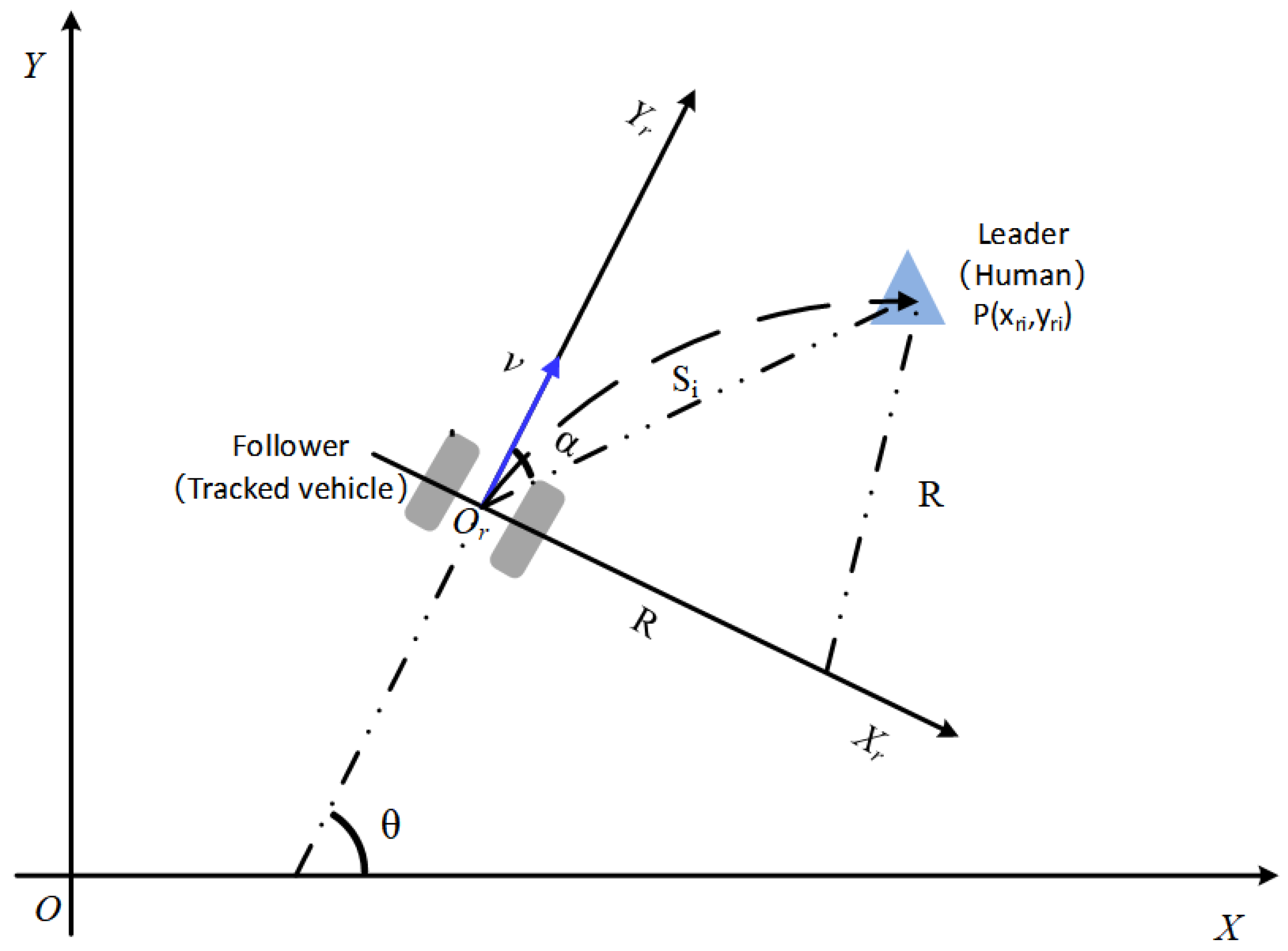
2.1. Leader-Following Model

The fundamental task of the leader-following function is as follows: The leader (human) walks or runs at will on the ground, while the unmanned tracked vehicle carries supplies and autonomously follows the leader. Two coordinate systems are established: one fixed on the ground as the geodetic coordinate system $OXY$ and the other fixed on the unmanned tracked vehicle as the follower coordinate system $O_r{X}_r{Y}_r$. In the follower coordinate system, $O_r$ is located at the geometric center of the tracked vehicle, with the $Y_r$-axis pointing toward the front of the vehicle and the $X_r$-axis pointing toward the right side of the vehicle. $\theta$ represents the angle between the $Y_r$-axis of the follower coordinate system and the X-axis of the geodetic coordinate system while R denotes the steering radius of the arc trajectory as the tracked vehicle travels toward the leader. The leader-following motion and coordinate systems are shown in Figure 1.

The coordinates of the leader in the geodetic coordinate system vary arbitrarily based on the basic characteristics of leader motion. The unmanned tracked vehicle needs to obtain the relative coordinate position $X_{ri}$ and $Y_{ri}$ of the leader in $O_r{X}_r{Y}_r$ through its leader detection unit and then reasonably control its speed and curvature through the motion control unit, so that the unmanned tracked vehicle can consistently follow the leader. During the following, the head of the vehicle is oriented toward the leader as far as possible, and the position of the vehicle closely follows the coordinates in the geodetic coordinate system as accurately as possible, ensuring a reasonable distance between the vehicle and the leader [33]. During the following, it is required that $X_r$ approaches 0 and $Y_r$ remains within a reasonable range based on the leader’s speed. When the leader abruptly stops, the tracked vehicle must promptly respond to ensure a safe braking distance. The specific tracking targets are as follows:

$$\left\{\begin{array}{c}{x}_{ri}\to 0\hfill \\ y_{ri}\to \left|\mathsf{\Phi }\right|\hfill \\ \mathsf{\Phi }=f\left(x_{ri},y_{ri},{\dot{x}}_{ri},{\dot{y}}_{ri},v\right)\hfill \end{array}\right.$$

(1)

where $\mathsf{\Phi }$ represents the optimal preset following distance to the leader, and its value is dependent on the leader’s speed (${\dot{x}}_{ri}$,${\dot{y}}_{ri}$); v is the current speed of the tracked vehicle. The parameters can be adjusted based on actual conditions to make the following distance more reasonable.

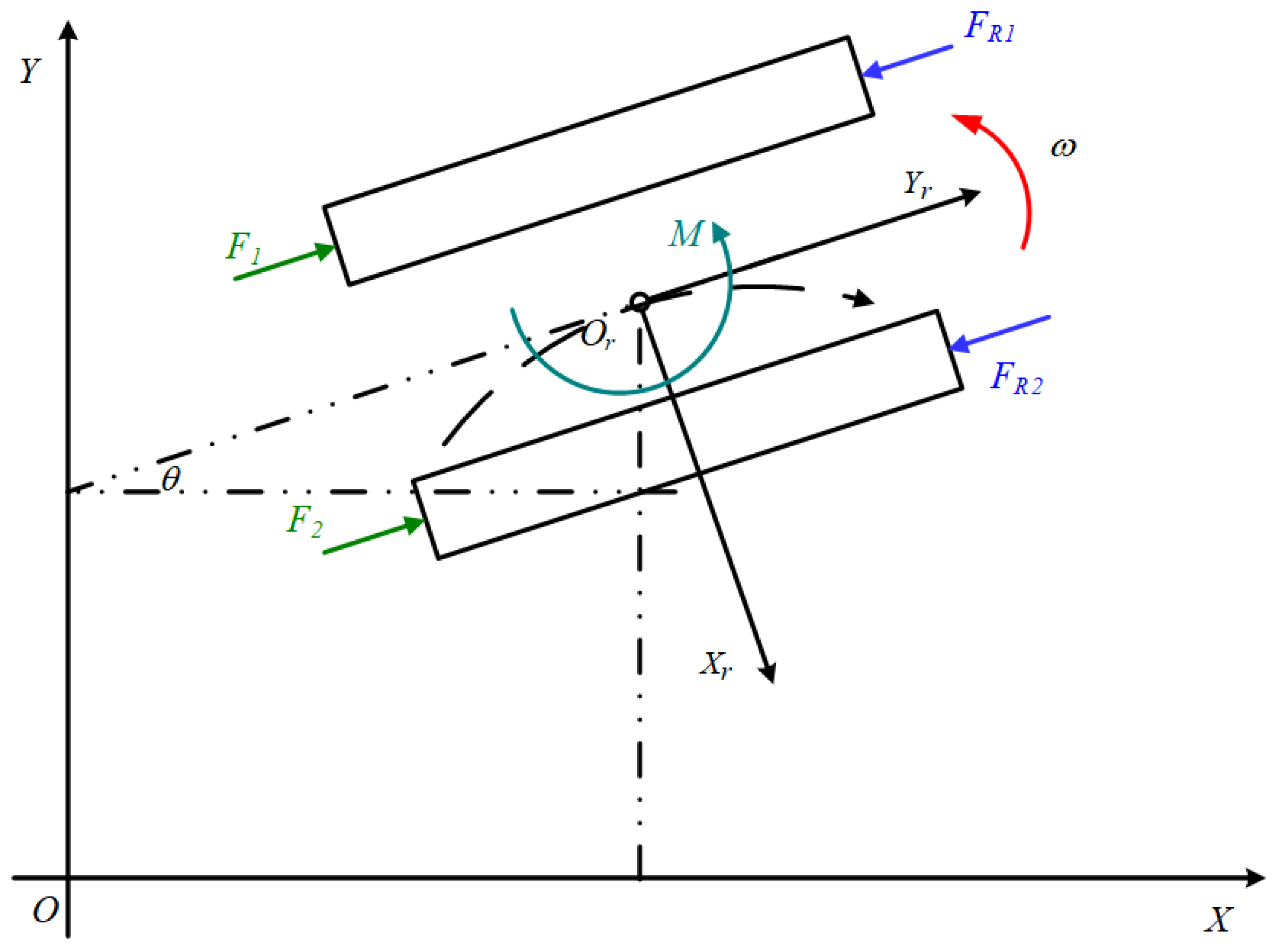
2.2. Dynamics Model of the Tracked Vehicle

As mentioned above, the geodetic coordinate system is denoted as $OXY$, and the follower coordinate system of the tracked vehicle is denoted as $O_r{X}_r{Y}_r$. The resultant forces acting on the tracked vehicle are shown in Figure 2.

In Figure 2, $\omega$ is the steering angular velocity, M is the steering resistance torque, $F_1$ and $F_2$ are the tractive force of the left and right tracks, and $F_{R1}$ and $F_{R2}$ are the rolling resistance of each track. The dynamics model of the tracked vehicle is as follows [14]:

$$\left\{\begin{array}{c}m\dot{v}=F_1+F_2-F_{R1}-F_{R2}\hfill \\ J\dot{\omega }=\left(F_2-F_1\right)·\frac{B}{2}-M\hfill \\ M=\frac{{\mu }_{max}mgL}{4\left(0.925 + 0.15\rho \right)}\hfill \\ \rho =\frac{1}{\tau B}=\frac{v}{B\omega }\hfill \\ \left|F_1\right|\le \phi N_1,\hspace{1em}\left|F_2\right|\le \phi N_2\hfill \\ F_{R1}+F_{R2}=fmg\hfill \end{array}\right.$$

(2)

where $\rho$ represents the relative steering radius; v is the vehicle’s center velocity; $\tau$ is the curvature, which is the reciprocal of the steering radius; m is the total vehicle mass; J is the moment of inertia; L is the track contact length; B is the center track distance; ${\mu }_{max}$ is the steering resistance coefficient for a specific road surface; $\phi$ is the adhesion coefficient; f is the rolling resistance coefficient; and $N_1$ and $N_2$ are the ground pressures on the left and right tracks. To simplify the calculations, the rolling resistance experienced by the left and right tracks is considered as a whole.

It is worth noting that the driving force of the vehicle is provided by the motor [34]:

$$F_{\mathrm{i}}=\frac{T_{e\mathrm{i}}{i}_c}{r_z}$$

(3)

where the corner marks $\mathrm{i}=1,2$, respectively, denoting the left and right sides; $T_{e\mathrm{i}}$ is the torque motor; $i_c$ is the gear ratio from the motor to the driving wheel; and $r_z$ is the driving wheel radius.

Additionally, the braking force provided by the motor is often constrained by its maximum braking torque and power, especially in emergency braking conditions, where hydraulic braking force may be required as a supplement. Considering the motor braking characteristics, a conventional braking force distribution strategy is adopted as follows [35]:

$$F_{\mathrm{brake}}=\left\{\begin{array}{cc}\frac{T_e{i}_c}{r_z},\hfill & F_{\mathrm{brake}}^{\ast }<F_{e\_max}\\ \frac{T_{e\_max}{i}_c}{r_z}+F_h,\hfill & F_{\mathrm{brake}}^{\ast }\ge F_{e\_max}\end{array}\right.$$

(4)

where $F_{\mathrm{brake}}$ is the actual braking force, $F_{e\_max}$ represents the maximum torque that the electric motor can provide, $F_{\mathrm{brake}}^{\ast }$ is the target braking force, and $F_h$ is the hydraulic braking force. When the target braking force is less than the maximum braking force that the electric motor can provide, the electric motor supplies all the braking force. When the target braking force is greater than or equal to the maximum braking force that the electric motor can provide, to ensure the safety of the vehicle braking, the electric motor outputs the maximum torque to provide the maximum braking force, with the remaining portion supplemented by hydraulic braking force.

2.3. Linear Equivalent Model

During the motion process, considerations primarily involve terrain changes and steering resistance coefficient variations, resulting in load fluctuations. Because the steering curvature can better reflect changes in the heading angle of tracked vehicles, aiding the vehicle in rapidly adjusting toward the leader, it is more suitable to choose the curvature as one of the state variables. Therefore, with the speed (v) and curvature ($\tau$) as the state variables, the dynamics model (2) is reconstructed as follows:

$$\left\{\begin{array}{c}\dot{v}=\frac{F_1 + F_2}{m}-f\mathrm{g}\hfill \\ \dot{\tau }=\left(\frac{\left(F_2 - F_1\right)B}{2J}-\frac{M}{J}\right)·\frac{1}{v}-\left(\frac{F_1 + F_2}{m}-f\mathrm{g}\right)·\frac{\tau }{v}\hfill \\ M=\frac{{\mu }_{max}mgL}{4\left(0.925 + \frac{0.15}{\tau B}\right)}\hfill \end{array}\right.$$

(5)

The MRAC we chose generally requires the controlled object to be a linear, single-input, single-output scleronomous system. It is necessary to process the dynamics model separately with v and $\tau$ as the state variables to obtain the equivalent inputs $F_v$ and $F_{\tau }$ for an adaptive feedback control system. Therefore, by performing a Taylor expansion of the steering resistance torque M at point ${\tau }_0$, we have:

$$M=\frac{{\mu }_{max}mgLB\tau }{3.7B\tau +0.6}=\frac{{\mu }_{max}mgL}{3.7}·\left({\left(\frac{3.7B{\tau }_0}{3.7B{\tau }_0+0.6}\right)}^2+\left(\frac{0.6·3.7B}{{\left(3.7B{\tau }_0+0.6\right)}^2}\right)\tau \right)$$

(6)

The actual steering process can be viewed as combining many small segments of $\tau$, each representing a first-order linear steady-state equation under a specific ${\tau }_0$. Therefore, combining with (5) and (6), the dynamics model is reformulated as follows:

$$\left\{\begin{array}{c}\dot{v}={\psi }_1{F}_v-{\psi }_{2}v\hfill \\ \dot{\tau }={\zeta }_1{F}_{\tau }-{\zeta }_2\tau \hfill \\ F_v=\frac{F_1 + F_2}{m}-f\mathrm{g}\hfill \\ {\psi }_1=1\hfill \\ {\psi }_2=0\hfill \\ F_{\tau }=\frac{\left(F_2 - F_1\right)B}{2Jv}-\frac{1}{Jv}·\frac{{\mu }_{max}mgL}{3.7}·{\left(\frac{3.7B{\tau }_0}{3.7B{\tau }_0 + 0.6}\right)}^2\hfill \\ {\zeta }_1=1\hfill \\ {\zeta }_2=\frac{1}{Jv}·\frac{{\mu }_{max}mgL}{3.7}·\left(\frac{0.6·3.7B}{{\left(3.7B{\tau }_0 + 0.6\right)}^2}\right)+\left(\frac{F_1 + F_2}{mv}-\frac{f\mathrm{g}}{v}\right)\hfill \end{array}\right.$$

(7)

where $F_v$ and $F_{\tau }$ are equivalent inputs to the system, as they are only related to the actual control inputs $F_1+F_2$ through constant terms. At this point, the construction of the linear equivalent model is achieved.

3. Control Strategy

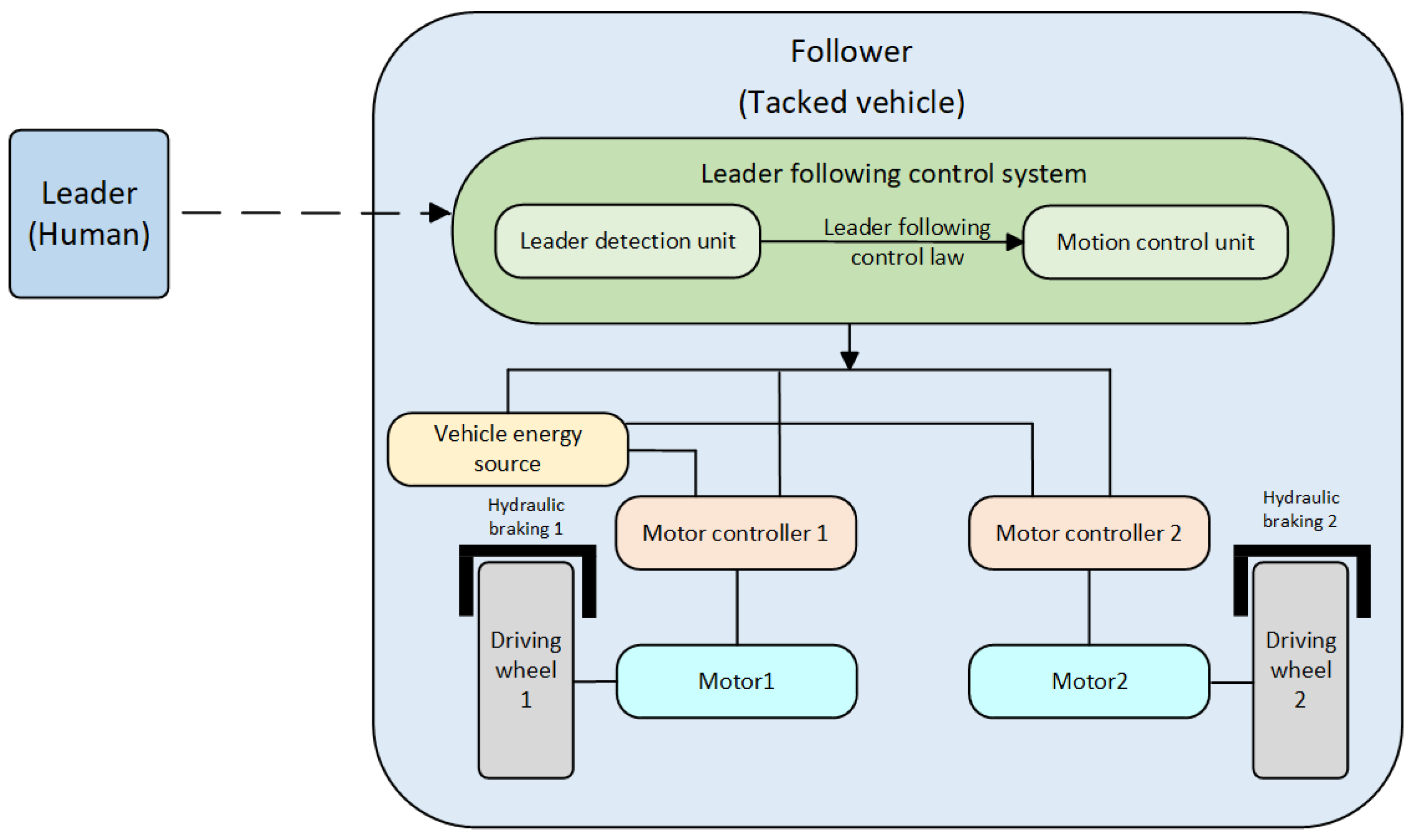
3.1. Integrated Control Algorithm Structure

The tracked vehicle’s motion is controlled through the combined action of lateral and longitudinal forces. A rational decoupling control strategy is necessary to improve the control precision and meet the requirements of the leader-following task. Moreover, in the actual control of the vehicle, such parameters as f and ${\mu }_{\max }$ are unknown and time-varying; especially, the steering resistance torque is in the unpredictable changes. Therefore, if an open-loop approach is used to calculate the target drive torque $T_i^{\ast }$, the adaptability of the strategy could be limited. So, it is crucial to design a closed-loop feedback control structure to improve the robustness and stability.

The adaptive control strategy devised in this study involves the following steps: First, the control signals from the leader detection unit are analyzed to extract the target vehicle speed ($v^{\ast }$) and the target steering curvature (${\tau }^{\ast }$). Then, both of them are subject to the closed-loop control in comparison with the actual vehicle speed (v) and steering curvature ($\tau$) so as to enable adaptive adjustment to the reasonable target driving force $F_i^{\ast }$.

Despite adopting a closed-loop control structure for v and $\tau$, there are still significant challenges in designing closed-loop algorithms for leader-following tasks. The main reasons include the following:

• The interaction mechanism between the tracks and the ground is highly complex, leading to such characteristics as indefinite inertia, unknown parameters, nonlinearity, and multiple-input multiple-output (MIMO) in the dynamics model of the tracked vehicles;
• Human behavior often exhibits significant uncertainties, such as sudden changes in speed and direction, so highly adaptive control algorithms are required;
• The strong coupling between v and $\tau$ results in mutual influences on the closed-loop control over the two parameters.

To address the above challenges, this study proposed a control strategy by employing the model reference adaptive control (MRAC), which utilizes the leader’s information and the vehicle’s feedback to adjust the control objectives. With a reference model for parameter-determined ideal vehicle dynamics used to estimate road loads, the motor torque is dynamically adjusted to ensure real-time tracking of the actual speeds and curvatures based on the reference model’s speed and curvature outputs. This adaptive closed-loop control is designed to achieve stable leader-following control. The control flowchart is shown in Figure 3, which indicates the reference system parameters with subscript “m” and the actual system parameters with subscript “p”.

The main components of the control structure include the “leader-following control law; computation of target speed and curvature; reference dynamics model; adaptive control law; and computation of target driving forces”. The specific solution process is as follows: Initially, to parse the leader’s signals, resolve them into $v^{\ast }$ and ${\tau }^{\ast }$; subsequently, based on $v^{\ast }$ and ${\tau }^{\ast }$, compute a set of $v_m$, $F_{vm}$, ${\tau }_m$, and $F_{{\tau }_m}$ in the speed control subsystem and the curvature control subsystem separately; then, using the adaptive control law module based on the reference vehicle speed and curvature, calculate the actual required values of $F_v$ and $F_{\tau }$; afterward, the adaptive solving system controls the required target driving forces $F_1^{\ast }$ and $F_2^{\ast }$, which are then transformed to obtain the target driving torques $T_1^{\ast }$ and $T_2^{\ast }$. These values are sent to the motor controller, hydraulic brake control valve, and other related devices, and the actual vehicle would operate under the control state at the speed of $v_p$ and steering curvature of ${\tau }_p$.

3.2. Leader-Following Control Law

As mentioned above, the leader-following control law is based on the relative coordinate position ($x_{ri}$ and $y_{ri}$) of the leader in $O_r{x}_r{y}_r$. The specific control law is as follows: If the leader is directly in front of the tracked vehicle, the vehicle will travel straight toward the leader; if the leader is not directly in front of the tracked vehicle (i.e., $y_{ri}$ is not close to 0), the unmanned vehicle will typically go along a smooth circular curve to the leader under a controlled state. Using curvatures instead of the steering radius for control can avoid the unmanageable situation that the steering radius value is infinite under the straight driving condition.

To ensure a reasonable following distance, i.e., to keep up with the leader while maintaining a safe distance, the target vehicle speed and curvature for the tracked vehicle shall be calculated in relation to the relative distance and speed between the leader and the vehicle. Thus, the control law of the target steering curvature (${\tau }^{\ast }$) and the target speed ($v^{\ast }$) is given by:

$$\left\{\begin{array}{c}{v}^{\ast }=k_1·\sqrt{{\dot{x}}_{ri}^2+{\dot{y}}_{ri}^2}+k_2·S_i\hfill \\ {\tau }^{\ast }=\frac{2sin\alpha }{S_i}=\frac{2sin\left(arctan\frac{x_{ri}}{y_{ri}}\right)}{\sqrt{x_{ri}^2 + y_{ri}^2}}\hfill \end{array}\right.$$

(8)

where $\alpha$ is the angle between the vehicle’s orientation and the following target at time i, $S_i$ is the position of the vehicle relative to the following target, $k_1$ is the current relative speed coefficient of the vehicle, and $k_2$ is the distance coefficient of the following target.

3.3. Reference Model

The purpose of constructing a reference model is to provide a standard or ideal performance benchmark for the control subsystem. This benchmark enables the control system to continuously adjust the actual speed and curvature of the tracked vehicle, ensuring that they closely track the reference model’s outputs in real time. Using (5), the reference dynamics model is designed as follows:

$$\left\{\begin{array}{c}{\dot{v}}_m=\frac{F_{1m} + F_{2m}}{m}-f\mathrm{g}\hfill \\ {\dot{\tau }}_m=\left(\frac{\left(F_{2m} - F_{1m}\right)B}{2J}-\frac{M}{J}\right)·\frac{1}{v}-\left(\frac{F_{1m} + F_{2m}}{m}-f\mathrm{g}\right)·\frac{\tau }{v_m}\hfill \\ M=\frac{{\mu }_{max}mgL}{4\left(0.925 + \frac{0.15}{{\tau }_{m}B}\right)}\hfill \end{array}\right.$$

(9)

This model is designed as a nonlinear dual-input and dual-output state-space system. The input variables of the system are $F_{1m}$ and $F_{2m}$, the state variables are $v_m$ and ${\tau }_m$, and the output variables of the system are $v_m$ and ${\tau }_m$. Other parameters can be preset as close to the vehicle’s actual conditions. Under the equilibrium condition of (9), the reference driving forces $F_{1m}$ and $F_{2m}$ are obtained as follows:

$$\left\{\begin{array}{c}{F}_{1m}=\left(\frac{f}{2}-\frac{{\mu }_{max}}{4B\left(0.925 + \frac{0.15}{{\tau }^{\ast }B}\right)}\right)·m\mathrm{g}\hfill \\ F_{2m}=\left(\frac{f}{2}+\frac{{\mu }_{max}}{4B\left(0.925 + \frac{0.15}{{\tau }^{\ast }B}\right)}\right)·m\mathrm{g}\hfill \end{array}\right.$$

(10)

Substitute the equivalent inputs into the reference model:

$${\dot{v}}_m={\psi }_{1m}{F}_{vm}-{\psi }_{2m}{v}_m,\hspace{1em}({\psi }_{2m}>0)$$

(11)

In addition, ${\psi }_{1m}$ and ${\psi }_{2m}$ (should be greater than zero) need to be designed based on closed-loop poles and stability margins to ensure the stability and rapid response of the reference system’s $v_m$ response. The system is also a scleronomous system.

Similar processing is applied to the actual system, and the following results can be obtained:

$${\dot{v}}_p={\psi }_{1p}{F}_{vp}-{\psi }_{2p}{v}_p$$

(12)

where ${\psi }_{1p}$ and ${\psi }_{2p}$ are determined by the actual terrain and are generally not equal to the values of the corresponding parameters in the reference system. Due to these differences, we need to design an adaptive algorithm to eliminate the influence and ensure the system’s robustness. Of course, if the values of the reference system are very close to the actual system, the difficulty of adapting the algorithm to adjust the parameters will be lower.

The algorithm design for the equivalent input of the dynamics equations with the vehicle speed as the state variable is based on excluding constant terms to ensure closed-loop pole placement:

$$F_{vm}=\frac{F_{1m}+F_{2m}}{m}-f\mathrm{g}$$

(13)

Similar handling is applied to the reference system for the curvature, resulting in:

$${\dot{\tau }}_m={\zeta }_{1m}{F}_{\tau m}-{\zeta }_{2m}{\tau }_m,\hspace{1em}({\zeta }_{2m}>0)$$

(14)

In addition, ${\zeta }_{1m}$ and ${\zeta }_{2m}$ (should be greater than zero) need to be designed based on closed-loop poles and stability margins to ensure the stability and rapid response of the reference system’s ${\tau }_m$ response. The system is also a scleronomous system. Similar processing is applied to the actual system, the actual dynamics model, and the following results can be obtained:

$${\dot{\tau }}_p={\zeta }_{1p}{F}_{\tau p}-{\zeta }_{2p}{\tau }_p$$

(15)

where ${\zeta }_{1p}$ and ${\zeta }_{2p}$ are determined by the actual environment and are generally not equal to the values of the corresponding parameters in the reference system. Similarly, an adaptive algorithm is designed to eliminate their influence and ensure the robustness of the system.

The following is the algorithm for the equivalent input of the dynamics equation with the curvature as the state variable:

$$F_{{\tau }_m}=\frac{\left(F_{2m}-F_{1m}\right)B}{2J{v}_m}-\frac{1}{J{v}_m}·\frac{{\mu }_{max}mgL}{3.7}·{\left(\frac{3.7B{\tau }_m}{3.7B{\tau }_m+0.6}\right)}^2$$

(16)

Due to the skillful design of $F_{vm}$ and $F_{\tau m}$, it ensures that $v_m$ = $v^{\ast }$ and ${\tau }_m$ = ${\tau }^{\ast }$, thereby achieving the tracking of the reference system response to the leader-following control intentions.

3.4. Motion Adaptive Control Law

The purpose of designing the adaptive control law is to determine the actual inputs $F_{vp}$ and $F_{\tau p}$ required for controlling the adaptive solving system based on $F_v$, $F_{\tau }$, $v_m$, and ${\tau }_m$ and the feedback of the actual motor speed, ultimately deriving the motor torque.

The closed-loop control method of the subsystem is shown in Figure 4.

The adaptive algorithm for the speed closed-loop control with v as the state variable is as follows:

$$\left\{\begin{array}{c}{F}_{vp}={\chi }_1{F}_{v_m}+{\chi }_2{v}_p\hfill \\ e_v=v_p-v_m\hfill \\ {\dot{\chi }}_1=-k_v{e}_v{F}_{v_m}\hfill \\ {\dot{\chi }}_2=-k_v{e}_v{v}_p\hfill \end{array}\right.$$

(17)

where $e_v$ is the error between the reference speed subsystem $v_m$ and the actual speed subsystem $v_p$. The input $F_{vp}$ acts on the actual system, and the control result is that $e_v$ converges to zero, achieving the servo of $v_p$ to $v_m$. The parameters ${\chi }_1$ and ${\chi }_2$ are adaptively adjusted based on $e_v$, forming the control algorithm. When the error is significant, the change rate of ${\chi }_1$ and ${\chi }_2$ is significant, ensuring rapid error convergence. As the error approaches zero, the change rate of ${\chi }_1$ and ${\chi }_2$ becomes small, ensuring that the input $F_{vp}$ quickly stabilizes without oscillation.

Similarly, the adaptive algorithm for the speed closed-loop control with $\tau$ as the state variable is as follows:

$$\left\{\begin{array}{c}{F}_{\tau p}={\gamma }_1{F}_{\tau m}+{\gamma }_2{\tau }_p\hfill \\ e_{\tau }={\tau }_p-{\tau }_m\hfill \\ {\dot{\gamma }}_1=-k_{\tau }{e}_{\tau }{F}_{\tau m}\hfill \\ {\dot{\gamma }}_2=-k_{\tau }{e}_{\tau }{\tau }_p\hfill \end{array}\right.$$

(18)

where $e_{\tau }$ is the error between the reference curvature subsystem $v_m$ and the actual curvature subsystem $v_p$. $F_{vp}$ affects the input for the straight-line speed, while $F_{\tau p}$ influences the steering angular velocity. Utilizing these inputs, the target driving forces $F_1^{\ast }$ and $F_2^{\ast }$ are calculated with the following equations:

$$\left\{\begin{array}{c}{F}_{vp}=\frac{F_1^{\ast } + F_2^{\ast }}{m}-f\mathrm{g}\hfill \\ F_{\tau p}=\frac{\left(F_1^{\ast } - F_2^{\ast }\right)B}{2J{v}_p}-\frac{1}{J{v}_p}·\frac{{\mu }_{max}mgL}{3.7}·{\left(\frac{3.7B{\tau }_p}{3.7B{\tau }_p + 0.6}\right)}^2\hfill \end{array}\right.$$

(19)

Through the adjusting effect of the adaptive law, $e_v$ between $v_m$ and $v_p$ can rapidly converge to zero, and $e_{\tau }$ between ${\tau }_m$ and ${\tau }_p$ can also quickly converge to zero. These results in $v_p$ and ${\tau }_p$ closely follow $v_m$ and ${\tau }_m$, ensuring that the actual vehicle response effectively follows the response of the reference system. Thus, $v_p$ and ${\tau }_p$ can well track $v^{\ast }$ and ${\tau }^{\ast }$ under complex road conditions.

Furthermore, in the actual control process, the driving and braking forces of the tracked vehicle are distributed according to the distribution law mentioned before.

3.5. Proof of Control System Stability

Stability is a crucial characteristic for the regular operation of a system, and Lyapunov theory serves as a fundamental theoretical basis for proving system stability. Therefore, it is necessary to utilize Lyapunov theory to demonstrate the stability of the proposed control system in the final analysis. However, the leader-following control law is based on a linear look-up table, which does not affect the stability of the system and does not require extensive proof. In control subsystems, the primary considerations are the stability of $v_p$ and ${\tau }_p$. For the speed subsystem, according to (17), $e_v$, ${\chi }_1$, and ${\chi }_2$ are relative variables to $v_p$, and the Lyapunov function can be chosen as:

$$V(e_v,{\chi }_1,{\chi }_2)=\frac{e_v^2}{2}+\frac{{\psi }_{1p}}{2k_v}·{\left({\chi }_1-\frac{{\psi }_{1m}}{{\psi }_{1p}}\right)}^2+\frac{{\psi }_{1p}}{2k_v}·{\left({\chi }_2-\frac{{\psi }_{2p}-{\psi }_{2m}}{{\psi }_{1p}}\right)}^2$$

(20)

Its derivative value is:

$$\begin{array}{lll}\dot{V}\hfill & =& e_v{\dot{e}}_v+\frac{{\psi }_{1p}}{k_v}·\left({\chi }_1-\frac{{\psi }_{1m}}{{\psi }_{1p}}\right)·{\dot{\chi }}_1+\frac{{\psi }_{1p}}{k_v}·\left({\chi }_2-\frac{{\psi }_{2p} - {\psi }_{2m}}{{\psi }_{1p}}\right)·{\dot{\chi }}_2\\ & =& e_v\left({\dot{v}}_p-{\dot{v}}_m\right)-{\psi }_{1p}·\left({\chi }_1-\frac{{\psi }_{1m}}{{\psi }_{1p}}\right)·e_v{F}_{vm}-{\psi }_{1p}·\left({\chi }_2-\frac{{\psi }_{2p} - {\psi }_{2m}}{{\psi }_{1p}}\right)·e_v{v}_p\hfill \\ & =& e_v\left({\dot{v}}_p-{\dot{v}}_m\right)-\left({\psi }_{1p}{\chi }_1-{\psi }_{1m}\right)·e_v{F}_{vm}-\left({\psi }_{1p}{\chi }_2+{\psi }_{2m}-{\psi }_{2p}\right)·e_v{v}_p\hfill \\ & =& e_v\left({\psi }_{1p}{F}_{vp}-{\psi }_{2p}{v}_p-{\psi }_{1m}{F}_{vm}+{\psi }_{2m}{v}_m\right)-\left({\psi }_{1p}{\chi }_1-{\psi }_{1m}\right)·e_v{F}_{vm}\hfill \\ & & -\left({\psi }_{1p}{\chi }_2+{\psi }_{2m}-{\psi }_{2p}\right)·e_v{v}_p\\ & =& e_v\left({\psi }_{2m}{v}_m-{\psi }_{2m}{v}_p\right)\\ & =& -{\psi }_{2m}{e}_v^2\\ & <& 0\end{array}$$

(21)

Similarly, for the curvature subsystem according to (18), the Lyapunov function with $\tau$ as the state variable can be chosen as:

$$V(e_{\tau },{\gamma }_1,{\gamma }_2)=\frac{e_{\tau }^2}{2}+\frac{{\zeta }_{1p}}{2k_{\tau }}·{\left({\gamma }_1-\frac{{\zeta }_{1m}}{{\zeta }_{1p}}\right)}^2+\frac{{\zeta }_{1p}}{2k_{\tau }}·{\left({\gamma }_2-\frac{{\zeta }_{2p}-{\zeta }_{2m}}{{\zeta }_{1p}}\right)}^2$$

(22)

Its derivative value is:

$$\begin{array}{lll}\dot{V}\hfill & =\hfill & e_{\tau }{\dot{e}}_{\tau }+\frac{{\zeta }_{1p}}{k_{\tau }}·\left({\gamma }_1-\frac{{\zeta }_{1m}}{{\zeta }_{1p}}\right)·{\dot{\gamma }}_1+\frac{{\zeta }_{1p}}{k_{\tau }}·\left({\chi }_2-\frac{{\zeta }_{2p} - {\zeta }_{2m}}{{\zeta }_{1p}}\right)·{\dot{\gamma }}_2\hfill \\ & =& e_{\tau }\left({\dot{\tau }}_p-{\dot{\tau }}_m\right)-{\zeta }_{1p}·\left({\gamma }_1-\frac{{\zeta }_{1m}}{{\zeta }_{1p}}\right)·e_{\tau }{F}_{\tau m}-{\zeta }_{1p}·\left({\gamma }_2-\frac{{\zeta }_{2p} - {\zeta }_{2m}}{{\zeta }_{1p}}\right)·e_{\tau }{\tau }_p\hfill \\ & =& e_{\tau }\left({\dot{\tau }}_p-{\dot{\tau }}_m\right)-\left({\zeta }_{1p}{\gamma }_1-{\zeta }_{1m}\right)·e_{\tau }{F}_{\tau m}-\left({\zeta }_{1p}{\gamma }_2+{\zeta }_{2m}-{\zeta }_{2p}\right)·e_{\tau }{\tau }_p\hfill \\ & =& e_{\tau }\left({\zeta }_{1p}{F}_{\tau p}-{\zeta }_{2p}{\tau }_p-{\zeta }_{1m}{F}_{\tau m}+{\zeta }_{2m}{\tau }_m\right)-\left({\zeta }_{1p}{\gamma }_1-{\zeta }_{1m}\right)·e_{\tau }{F}_{\tau m}\hfill \\ & & -\left({\zeta }_{1p}{\gamma }_2+{\zeta }_{2m}-{\zeta }_{2p}\right)·e_{\tau }{\tau }_p\\ & =& e_{\tau }\left({\zeta }_{2m}{\tau }_m-{\zeta }_{2m}{\tau }_p\right)\\ & =& -{\zeta }_{2m}{e}_{\tau }^2\\ & <& 0\end{array}$$

(23)

Thus, the subsystems’ stability is proved.

4. Experimental Results

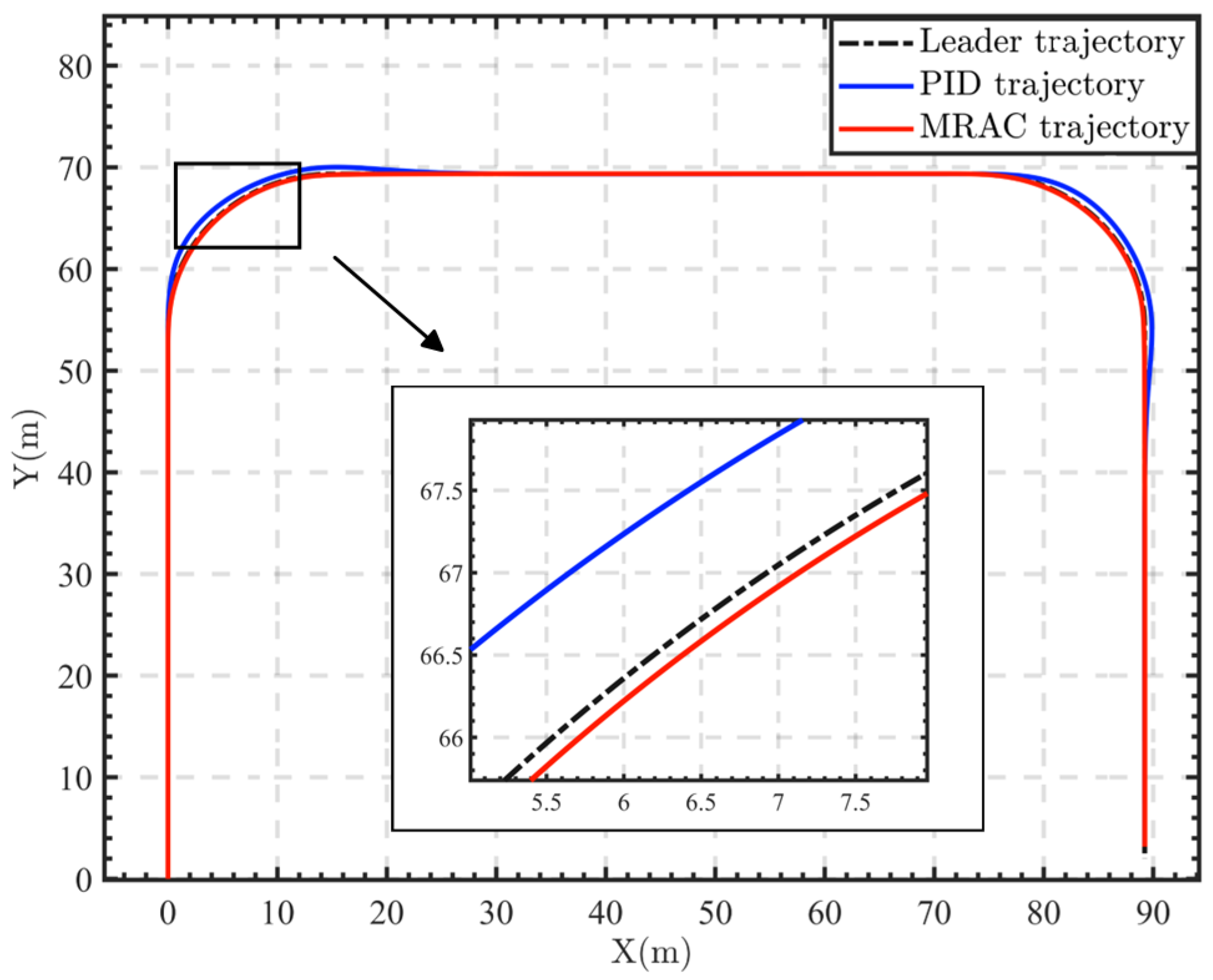
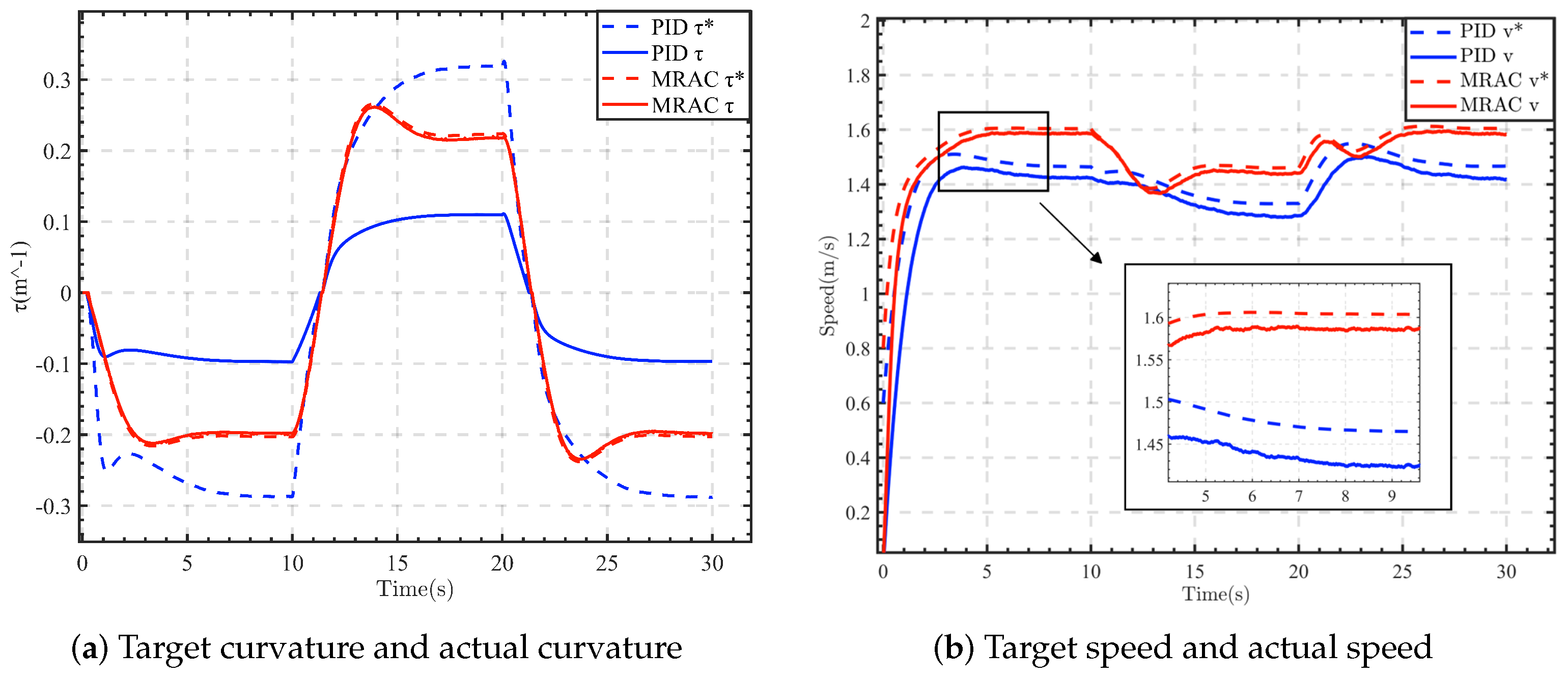
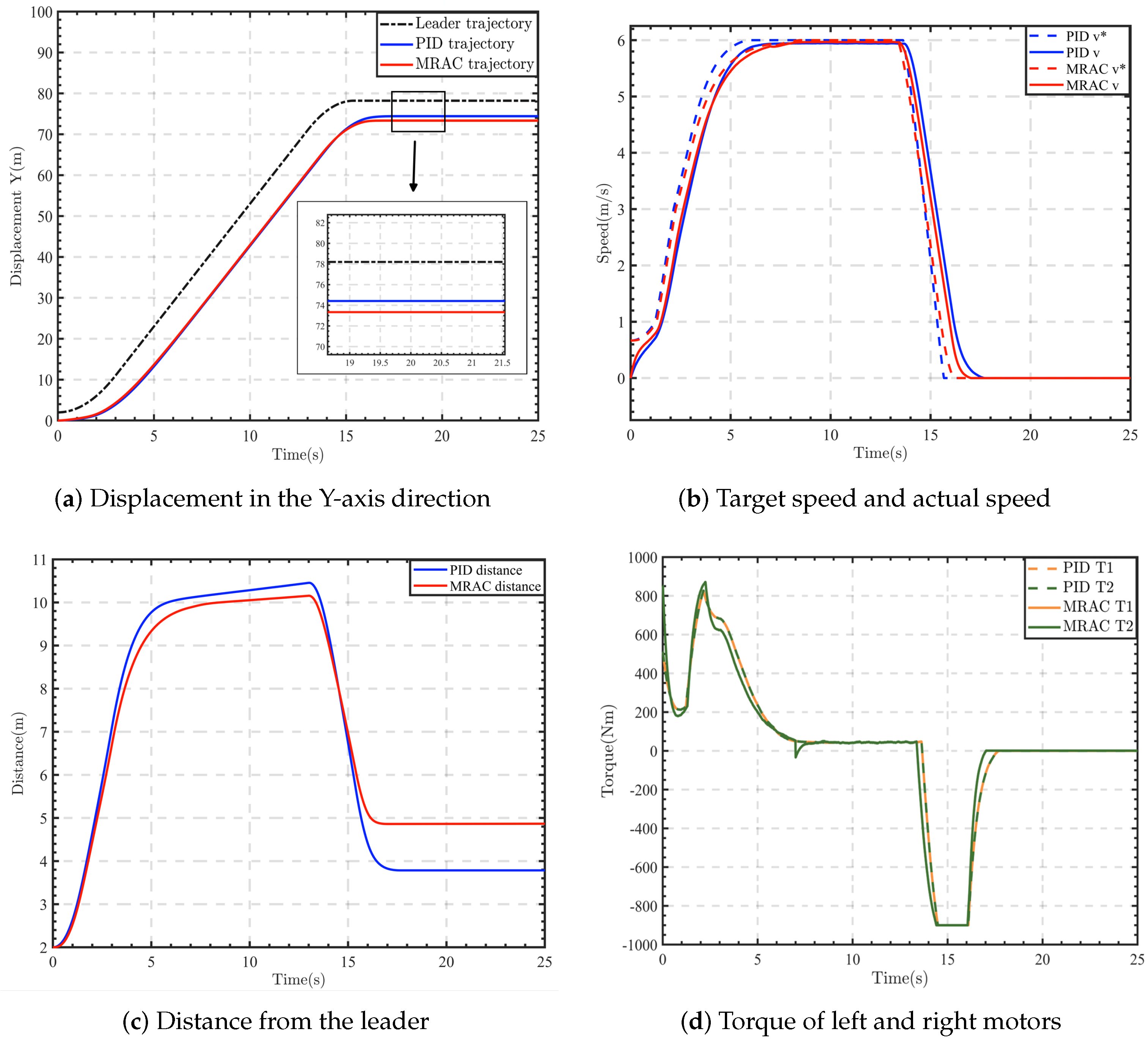
4.1. Simulation Validation

The simulations were performed using Matlab/Simulink and RecurDyn to validate the effectiveness of the proposed algorithm for the leader-following task, as shown in Figure 5. Three different conditions were designed to include straight-line driving combined with turning, continuous turning, and emergency braking, thereby covering the principal motion scenarios of the leader-following task. Furthermore, a comparative analysis was conducted on the simulation results between the MRAC control strategy proposed in this paper and the traditional PID control strategy. The simulation model is constructed based on the actual parameters of the platform, with its main parameters as shown in

Table 1. Simulation model parameters.

Vehicle Parameters
Weight/kg	8000
Track contact length/m	2.12
Driving wheel radius/m	0.26
Center track distance/m	1.78
Moment of inertia/kg·m2	1000
Gear ratio	9.83

.

4.1.1. Condition 1

Condition 1 involves the general movements of unmanned tracked vehicles in the leader-following task, including linear acceleration, deceleration, and constant-speed turning. The leader starts from a position 2 m away from the tracked vehicle. Within the first 10 s, the leader first performs a uniform acceleration motion in the positive y-axis direction at a speed of 2 m/s², then maintains a uniform motion at a speed of 7 m/s, and then reduces the speed to 2.5 m/s. From 10 s to 20 s, a constant angular velocity is applied for a clockwise steering motion, resulting in a 90-degree turn with a steering radius of 15 m. From 20 s to 30 s, the vehicle undergoes another variable-speed motion, starting with acceleration, then a constant speed, and then deceleration, while facing the positive x-direction. In the subsequent 10 s (30 s to 40 s), a constant angular velocity is applied for another 90-degree clockwise steering motion with a steering radius of 15 m. Finally, from 40 s to 50 s, the vehicle undergoes variable-speed motion in the negative y-axis direction, with the initial acceleration, constant speed, and eventual deceleration until the speed reaches 0. The experimental results are shown in Figure 6.

Figure 6 illustrates the leader-following effect of the unmanned tracked vehicle in condition 1, and Figure 7 compares the performance of the two control methods in condition 1. Compared to the PID control method, the maximum deviation between the MRAC vehicle trajectory and the leader trajectory is reduced by 6%, there is a maximum curvature error reduction of 11% and a maximum speed error reduction of 5%, and the maximum following distance is reduced by 12%. Moreover, MRAC can fully exploit the performance of the vehicle’s dual motor. MRAC performs well in straight-line motion and closely follows the leader in the steering phases, demonstrating better completion of the leader-following task than the PID control method.

4.1.2. Condition 2

Condition 2 accounts for the continuous turning scenarios in the leader-following task. The leader starts from a position 2 m away from the tracked vehicle. In the first 10 s, the leader performs a clockwise steering motion with a constant angular velocity for a 180-degree turn with a steering radius of 5 m. From 10 s to 20 s, the leader executes a counterclockwise steering motion with a constant angular velocity for a 90-degree turn with a steering radius of 4.5 m. Finally, from 20 s to 30 s, the leader performs a clockwise steering motion with a constant angular velocity for a 180-degree turn with a steering radius of 5 m. The experimental results are shown in Figure 8.

Figure 8 illustrates the leader-following effect of the unmanned tracked vehicle in simulation condition 2, and Figure 9 compares the performance of the two control methods in condition 2. In this case, the maximum deviation between the MRAC vehicle trajectory and the leader trajectory is reduced by 6.6%, there is a maximum curvature error reduction of 47% and a maximum speed error reduction of 3.5%, and the maximum following distance is reduced by 16%. Because this scenario involves low-speed control, the speed errors for both control methods are relatively small. It can be observed that the MRAC decoupling control method significantly improves the steering performance of the vehicle, even in extreme steering conditions where the PID curvature control deviation is significant, ensuring perfect following of the target curvature.

4.1.3. Condition 3

The condition of emergency braking is set up to verify the effectiveness of the proposed control algorithm in coping with unexpected situations. In this condition, the leader starts from a position 2 m away from the tracked vehicle. In the first 15 s, the leader undergoes a variable-speed motion with the initial acceleration followed by a constant speed, where the acceleration is 2 m/s². At 15 s, the leader abruptly stops. In the event of an abrupt stop by the leader, the unmanned tracked vehicle should promptly apply the brakes and maintain a safe distance to avoid collisions. The experimental results are shown in the Figure 10.

Figure 10 compares the performance of the two control methods in test condition 3. Due to the condition involving straight-line driving and emergency braking, only the displacement in the Y-axis direction needs to be considered. During regular driving phases, both control methods can effectively follow the leader’s movements. In the emergency braking phase, the MRAC control method achieves a reduction of 22% in the braking distance, enabling it to stop at a greater distance from the leader, ensuring the safety of the leader (human). Simultaneously, during the braking process, energy recovery can be achieved through the motor, reducing the vehicle’s energy consumption.

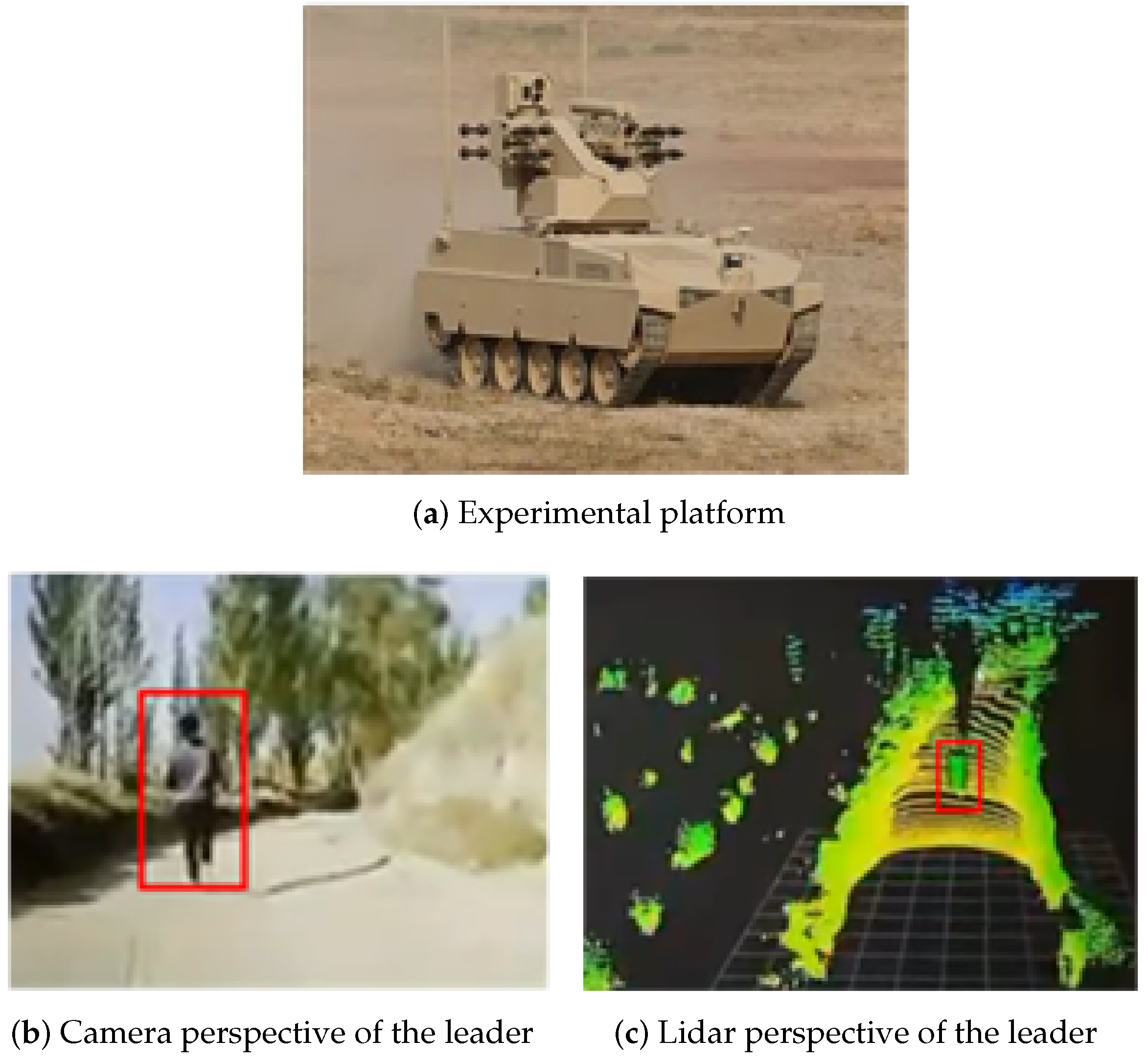
4.2. Experimental Validation

To validate the proposed control method, the experiments were conducted on a platform featuring a dual-motor-driven unmanned tracked vehicle equipped with cameras, Lidar, and inertial navigation. The overall vehicle’s topology is shown in Figure 11. The leader-following control system of the unmanned tracked vehicle consists of the leader detection unit and the motion control unit. The leader detection unit utilizes sensors and leader perception algorithms to obtain the leader’s relative coordinates ($x_{ri}$, $y_{ri}$) and sends this information to the motion control unit. The motion control unit initially calculates the obtained information ($x_{ri}$ and $y_{ri}$) into target speed and target curvature commands. Subsequently, based on the motion adaptive control algorithm, it further adjusts the vehicle’s drive and brake execution units. Finally, the adjusted commands are sent to the motor controller and control valve for execution via the CAN bus. The main parameters of the experimental platform are presented in

Table 2. Platform parameters.

Vehicle Parameters
Weight/kg	8000
Track contact length/m	2.12
Driving wheel radius/m	0.26
Center track distance/m	1.78
Gear ratio	9.83
Motor Parameters
Rated voltage/V	550
Rated rotational speed/rpm	1500
Peak rotational speed/rpm	4500
Rated torque/Nm	525
Peak torque/Nm	900

. However, the parameter for rotational inertia is not included due to the difficulty in accurately obtaining it.

The experimental platform and visualization results are shown in Figure 12. In order to make the experimental results more intuitive, the leader is marked with a red box.

In the actual vehicle experiment, the expected motion of the leader (human) is as follows: starting from a position 5 m away from the tracked vehicle, moving forward along the x-axis for 20 m, and then initiating a counterclockwise steering motion of 180 degrees with a steering radius of 10 m. However, during the actual experiment, due to the inability of the human leader to control his movement position precisely, there is a deviation between the actual trajectory of the leader and the expected trajectory. However, as this research focuses on leader-following rather than trajectory tracing, the primary objective is for the unmanned tracked vehicle to effectively trail the real-time movement of the leader. It is worth noting that this experiment lasted for a long period, and only the previously mentioned process of the leader’s movement was recorded as the starting and ending point of the experimental results, and the results are shown in Figure 13 and Figure 14.

Figure 14 illustrates the leader-following effect of the unmanned tracked vehicle under actual vehicle experiment conditions. In the experiment, the maximum deviation between the MRAC vehicle trajectory and the leader trajectory is 0.48 m, and the maximum curvature error is 0.05 m⁻¹. It can be observed that during straight-line movement, the following distance is positively correlated with the actual speed. During large curvature turning, the following distance is extended by approximately 0.5 m but remains within a controllable range. Therefore, in real-world scenarios, the control strategy utilized in this study can effectively control the vehicle, accomplishing the leader-following task excellently.

5. Conclusions

Due to the high precision required for motion control and the complex dynamic characteristics of unmanned tracked vehicles, achieving the leader-following task presents significant challenges. To address this issue, this paper decouples the leader-following control into speed and curvature control, utilizing model reference adaptive control (MRAC) to set up speed and curvature subsystems separately. The actual speed and curvature are continuously adjusted based on the reference model’s speed and curvature to achieve adaptive closed-loop control. The method demonstrates a significant performance improvement in the leader-following task for unmanned tracked vehicles through simulations and experiments. Compared with the traditional PID control method, the results show that the maximum following distance has been reduced by at least approximately 12% (ensuring the ability to keep up with the leader), the braking distance has effectively decreased by 22% (ensuring a safe distance in the emergency braking scenario and improving energy recovery), the curvature tracking accuracy has improved by at least 11% (improving steering performance), and the speed tracking accuracy has increased by at least 3.5% (improving following performance).

References

1. Amer, N.H.; Zamzuri, H.; Hudha, K.; Kadir, Z.A. Modelling and control strategies in path tracking control for autonomous ground vehicles: A review of state of the art and challenges. J. Intell. Robot. Syst. 2017, 86, 225–254. [Google Scholar]
2. Nguyen, V.L.; Kim, D.H.; Le, V.S.; Jeong, S.K.; Lee, C.H.; Kim, H.K.; Kim, S.B. Positioning and trajectory tracking for caterpillar vehicles in unknown environment. Int. J. Control Autom. Syst. 2020, 18, 3178–3193. [Google Scholar]
3. Sabiha, A.D.; Kamel, M.A.; Said, E.; Hussein, W.M. Dynamic modeling and optimized trajectory tracking control of an autonomous tracked vehicle via backstepping and sliding mode control. Proc. Inst. Mech. Eng. Part I J. Syst. Control Eng. 2022, 236, 620–633. [Google Scholar]
4. Li, R.; Fan, J.J.; Han, Z.D.; Guan, S.; Qin, Z.B. Configuration design and control of hybrid tracked vehicle with three planetary gear sets. J. Cent. South Univ. 2021, 28, 2105–2119. [Google Scholar] [CrossRef]
5. Hu, K.; Cheng, K. Trajectory Planning for an Articulated Tracked Vehicle and Tracking the Trajectory via an Adaptive Model Predictive Control. Electronics 2023, 12, 1988. [Google Scholar] [CrossRef]
6. Li, R.; Xiang, C.; Wang, C.; Fan, J.; Liu, C. Robust Adaptive Trajectory Tracking Control Approach for Autonomous Tracked Vehicles. Acta Armamentarii 2021, 42, 1128–1137. [Google Scholar]
7. Zhao, Z.; Liu, H.; Chen, H.; Hu, J.; Guo, H. Kinematics-aware model predictive control for autonomous high-speed tracked vehicles under the off-road conditions. Mech. Syst. Signal Process. 2019, 123, 333–350. [Google Scholar] [CrossRef]
8. Wang, P.; Rui, X.; Yu, H. Study on dynamic track tension control for high-speed tracked vehicles. Mech. Syst. Signal Process. 2019, 132, 277–292. [Google Scholar] [CrossRef]
9. Qin, Z.; Chen, L.; Fan, J.; Xu, B.; Hu, M.; Chen, X. An improved real-time slip model identification method for autonomous tracked vehicles using forward trajectory prediction compensation. IEEE Trans. Instrum. Meas. 2021, 70, 1–12. [Google Scholar] [CrossRef]
10. Kang, Y.; Zhang, Y.; Zeng, R. Path Tracking Control of Tracked Vehicles Considering Skid-steer Characteristic on Uneven Terrain. J. Cent. South Univ. 2022, 53, 491–501. [Google Scholar]
11. Lu, J.; Liu, H.; Guan, H.; Li, D.; Chen, H.; Liu, L. Trajectory Tracking Control of Unmanned Tracked Vehicles Based on Adaptive Dual-Parameter Optimization. Acta Armamentarii 2023, 44, 960–971. [Google Scholar]
12. Gai, J.; Liu, C.; Ma, C.; Shen, H. Steering control of electric drive tracked vehicle considering tracks’ skid and slip. Acta Armamentarii 2021, 42, 2092–2101. [Google Scholar]
13. Wang, B.Y.; Gong, J.W.; Gao, T.Y.; Zhang, R.Z.; Chen, H.Y.; Xi, J.Q. Longitudinal and lateral path following coordinated control method of tracked vehicle based on double-layer driver model. Acta Armamentarii 2018, 39, 1675–1682. [Google Scholar]
14. Tang, Z.; Liu, H.; Xue, M.; Chen, H.; Gong, X.; Tao, J. Trajectory Tracking Control of Dual Independent Electric Drive Unmanned Tracked Vehicle Based on MPC-MFAC. Acta Armamentarii 2023, 44, 129–139. [Google Scholar]
15. Hu, J.; Hu, Y.; Chen, H.; Liu, K. Research on trajectory tracking of unmanned tracked vehicles based on model predictive control. Acta Armamentarii 2019, 40, 456–563. [Google Scholar]
16. Sebastian, B.; Ben-Tzvi, P. Active disturbance rejection control for handling slip in tracked vehicle locomotion. J. Mech. Robot. 2019, 11, 021003. [Google Scholar] [CrossRef]
17. Han, J.; Wang, F.; Wang, Y. A control method for the differential steering of tracked vehicles driven independently by a dual hydraulic motor. Appl. Sci. 2022, 12, 6355. [Google Scholar] [CrossRef]
18. Mahalingam, I.; Padmanabhan, C. An integrated three-dimensional powertrain-vehicle dynamics model for tracked vehicle analysis. Proc. Inst. Mech. Eng. Part D J. Automob. Eng. 2023, 237, 3353–3366. [Google Scholar] [CrossRef]
19. Dasgupta, S.; Raghuraman, V.; Choudhury, A.; Teja, T.N.; Dauwels, J. Merging and splitting maneuver of platoons by means of a novel PID controller. In Proceedings of the 2017 IEEE Symposium Series on Computational Intelligence, Honolulu, HI, USA, 27 November–1 December 2017; pp. 1–8. [Google Scholar] [CrossRef]
20. Akopov, A.S.; Beklaryan, L.A.; Thakur, M. Improvement of Maneuverability within a Multiagent Fuzzy Transportation System with the Use of Parallel Biobjective Real-Coded Genetic Algorithm. IEEE Trans. Intell. Transp. Syst. 2022, 23, 12648–12664. [Google Scholar] [CrossRef]
21. Liang, J.; Li, Y.; Yin, G.; Xu, L.; Lu, Y.; Feng, J.; Shen, T.; Cai, G. A MAS-Based Hierarchical Architecture for the Cooperation Control of Connected and Automated Vehicles. IEEE Trans. Veh. Technol. 2023, 72, 1559–1573. [Google Scholar] [CrossRef]
22. Cosgun, A.; Florencio, D.A.; Christensen, H.I. Autonomous person following for telepresence robots. In Proceedings of the 2013 IEEE International Conference on Robotics and Automation, Karlsruhe, Germany, 6–10 May 2013; pp. 4335–4342. [Google Scholar]
23. Satake, J.; Chiba, M.; Miura, J. A SIFT-based person identification using a distance-dependent appearance model for a person following robot. In Proceedings of the 2012 IEEE International Conference on Robotics and Biomimetics (ROBIO), Guangzhou, China, 11–14 December 2012; pp. 962–967. [Google Scholar]
24. Evseev, K.B.; Kositsyn, B.B.; Kotiev, G.O.; Stadukhin, A.A.; Smirnov, I.A.; Godzhaev, Z.A. Design of the double-jointed multi-tracked vehicle steering control law providing its motion along a reference trajectory. J. Phys. Conf. Ser. 2021, 2032, 012064. [Google Scholar] [CrossRef]
25. Cui, D.; Wang, G.; Zhao, H.; Wang, S. Research on a Path-Tracking Control System for Articulated Tracked Vehicles. Stroj. Vestn. J. Mech. Eng. 2020, 66, 311–324. [Google Scholar] [CrossRef]
26. Shentu, S.; Xie, F.; Liu, X.J.; Gong, Z. Motion Control and Trajectory Planning for Obstacle Avoidance of the Mobile Parallel Robot Driven by Three Tracked Vehicles. Robotica 2021, 39, 1037–1050. [Google Scholar] [CrossRef]
27. Chunming, L.; Ke, B. Modeling and Analysis of Multi-level Coupling Dynamics of Tracked Vehicle Based on Load Transfer Path. J. Mech. Eng. 2023, 59, 157–174. [Google Scholar]
28. Xiong, H.; Chen, Y.; Li, Y.; Zhu, H.; Yu, C.; Zhang, J. Dynamic model-based back-stepping control design for-trajectory tracking of seabed tracked vehicles. J. Mech. Sci. Technol. 2022, 36, 4221–4232. [Google Scholar] [CrossRef]
29. Zou, T.; Angeles, J.; Hassani, F. Dynamic modeling and trajectory tracking control of unmanned tracked vehicles. Robot. Auton. Syst. 2018, 110, 102–111. [Google Scholar] [CrossRef]
30. Zheng, Q.; Tian, Y.; Deng, Y.; Zhu, X.; Chen, Z.; Liang, B. Reinforcement Learning-Based Control of Single-Track Two-Wheeled Robots in Narrow Terrain. Actuators 2023, 12, 109. [Google Scholar] [CrossRef]
31. Amokrane, S.B.; Laidouni, M.Z.; Adli, T.; Madonski, R.; Stanković, M. Active disturbance rejection control for unmanned tracked vehicles in leader–follower scenarios: Discrete-time implementation and field test validation. Mechatronics 2024, 97, 103114. [Google Scholar] [CrossRef]
32. Wang, S.; Guo, J.; Mao, Y.; Wang, H.; Fan, J. Research on the model predictive trajectory tracking control of unmanned ground tracked vehicles. Drones 2023, 7, 496. [Google Scholar] [CrossRef]
33. Wan, Q.; Li, Z.; Li, Y.; Ge, Z.; Wang, Y.; Wu, D. Target following method of mobile robot based on improved YOLOX. Acta Autom. Sin. 2023, 49, 1558–1572. [Google Scholar]
34. Zeng, G.; Wang, W.; Gai, J.; Ma, C.; Li, X.; Li, H. Steering on Ramp Control Strategy of Double Motor Coupling Drive Transmission for Tracked Vehicle. Acta Armamentarii 2021, 42, 2189–2195. [Google Scholar]
35. Zhang, L.; Liu, Q.; Wang, Z. Research on Electro-hydraulic Composite ABS Control for Four-wheel-independent-drive Electric Vehicles Based on Robust Integral Sliding Mode Control. J. Mech. Eng. 2022, 58, 243–252. [Google Scholar]
Figure 1. The schematic diagram of leader-following motion.
Wevj 15 00239 g001
Figure 2. Resultant forces acting on the tracked vehicle.
Wevj 15 00239 g002
Figure 3. Overall control flowchart.
Wevj 15 00239 g003
Figure 4. Closed-loop control method of subsystem.
Wevj 15 00239 g004
Figure 5. The simulation model of the tracked vehicle in RecurDyn.
Wevj 15 00239 g005
Figure 6. Schematic diagram of leader-following under condition 1.
Wevj 15 00239 g006
Figure 7. Performance comparison of two control methods under condition 1.
Wevj 15 00239 g007
Figure 8. Schematic diagram of leader-following under condition 2.
Wevj 15 00239 g008
Figure 9. Performance comparison of two control methods under condition 2.
Wevj 15 00239 g009aWevj 15 00239 g009b
Figure 10. Performance comparison of two control methods under condition 3.
Wevj 15 00239 g010
Figure 11. Topology structure of dual-motor-driven tracked vehicle.
Wevj 15 00239 g011
Figure 12. The experimental platform and visualization results.
Wevj 15 00239 g012
Figure 13. Schematic diagram of leader-following under actual vehicle experiment.
Wevj 15 00239 g013
Figure 14. Performance in actual vehicle experiments.
Wevj 15 00239 g014