Article

Research on a Multi-Strategy Improved Sand Cat Swarm Optimization Algorithm for Three-Dimensional UAV Trajectory Path Planning

1
School of Mechanical and Electrical Engineering, Xuzhou University of Technology, Xuzhou 221018, China
2
School of Electrical Engineering, China University of Mining and Technology, Xuzhou 221116, China
3
College of Electrical Engineering, Zhejiang University, Zheda Road 38, Hangzhou 310027, China
*
Author to whom correspondence should be addressed.
World Electr. Veh. J. 2024, 15(6), 244; https://doi.org/10.3390/wevj15060244
Submission received: 26 April 2024 / Revised: 23 May 2024 / Accepted: 27 May 2024 / Published: 31 May 2024

Abstract

:
In response to the issues of premature convergence, lack of population diversity, and poor convergence accuracy in the traditional Sand Cat Swarm Optimization (SCSO) algorithm, a Multi-Strategy Improved SCSO (MISCSO) algorithm is proposed. Firstly, multiple population strategies are used to avoid premature convergence and falling into local optima traps. Secondly, a distribution estimation learning strategy is introduced to represent the relationships between individuals, using probability models to improve algorithm performance. Next, the diversity of candidate solutions in the elite pool is utilized to expand the search space and enhance the algorithm’s ability to avoid local solutions. Lastly, a Cauchy disturbance strategy is adopted to accelerate the convergence speed of the algorithm, thereby improving the search efficiency and convergence accuracy. The experimental results of CEC2017 tests show that the improved algorithm balances convergence speed and global search capabilities effectively. Finally, the algorithm is applied to actual drone path planning and compared with six other intelligent algorithms, demonstrating the practicality and effectiveness of the improved algorithm.

1. Introduction

Unmanned Aerial Vehicles (UAVs) are extensively utilized in both military and civilian applications owing to their small size, high mobility, and ability to carry a variety of sensors. In the face of complex mission environments, successful mission completion by a UAV hinges on its ability to plan a path that is short-range, low in environmental threat cost, and conducive to flight capabilities. A superior path-planning algorithm not only ensures the optimality of the global path but also aids in obstacle avoidance and enhances the overall flight efficiency of the UAV. Consequently, experts worldwide have delved into the path planning problem of UAVs, with many utilizing conventional algorithms for path planning. For instance, Huang et al. [1] developed a method that incorporates a strategy for navigating around the nearest obstacle within an artificial potential field (APF). They introduced a parallel search algorithm that involves UAVs detecting obstacles in real-time while moving around the nearest obstacle to reach a target location. Simulation results were presented to showcase the effectiveness of the proposed path-planning algorithm and controller in action. Fu et al. [2] implemented a reinforcement learning approach using value functions to navigate unpredictable environments. This method is designed to optimize the path for reconnaissance and identification of points of interest. Simulations demonstrate the algorithm’s success in detecting targets in complex terrains with restrictions and efficiently returning to a specified endpoint for communication. Yuan et al. [3] enhanced the Lazy Theta* algorithm by refining neighbor node search, implementing a line-of-sight algorithm, and adjusting the heuristics weight to improve path planning for UAVs in complex environments with multiple constraints. Guo et al. [4] introduced the Flight Cost-based Rapidly exploring Random Tree star (FC-RRT*) algorithm, which integrates a cost function to generate optimal paths, prioritizing safety, path length, and flight constraints efficiently in complex environments. Li et al. [5] proposed the Improved Probabilistic Roadmap (IPRM) algorithm to tackle energy consumption challenges in multi-UAV path planning, achieving smoother and shorter paths with sampling of third-order B-spline curves for angle rotation. Li et al. [6] developed a 3D UAV path-planning model combining an enhanced A-star algorithm with an improved R5DOS intersection model, reducing computational complexity and calculation time in three-dimensional spaces. Wang et al. [7] presented an improved dynamic window approach (DWA) algorithm integrated with the 3D VFH+ algorithm to design a cooperative formation obstacle avoidance control algorithm, optimizing obstacle avoidance for UAV formation flight. Amylia et al. [8] introduced a hybrid optimization scheme merging Chaotic Aquila Optimization with Simulated Annealing, resulting in improved performance in minimizing fitness values across different scenarios by striking a balance between exploitation and exploration.
In real three-dimensional environments, path-planning algorithms not only require strong global planning capabilities but also need to possess effective local re-planning abilities for UAVs to navigate and avoid threats promptly in emergency situations. Different path-planning algorithms yield varying planning effects. To address limitations such as long search times, susceptibility to local optima, premature convergence, and low efficiency in shrinking feasible routes, researchers are increasingly turning to group intelligent algorithms for UAV path planning in 3D environments. Deng et al. [9] introduced an improved Particle Swarm Optimization (PSO) algorithm tailored for 3D path planning. This enhanced algorithm combines PSO with genetic algorithms, incorporates dynamic inertial weights, and integrates sigmoid functions to enhance genetic algorithm functions such as crossover and mutation probabilities. Simulation results demonstrate that the refined PSO algorithm achieves superior route planning outcomes, boasting faster and more stable performance. Chen et al. [10] introduced the TRS-Chimp Optimization Algorithm (TRS-ChOA) for optimizing 3D path planning. By incorporating a similarity preference weight, the algorithm prevents individuals from over-assimilating and escaping local optima, leading to reduced path length and improved fitness values in 3D environments. Zhang et al. [11] enhanced the Harris Hawks Optimization (HHO) algorithm with a Cauchy mutation strategy and adaptive weight, resulting in increased population diversity and optimized path planning results for UAVs. Rajeev Kumar et al. [12] proposed the RLV-Grey Wolf Optimization algorithm, utilizing reinforcement learning to adaptively control candidate operations for effective path planning in 3D environments. Dewangan et al. [13] introduced the Salp Swarm Algorithm (SSA) and demonstrated superior performance in UAV route planning in 3D environments compared to other algorithms, enhancing cost and time efficiencies. Wang et al. [14] presented an improved Tuna Swarm Optimization (TSO) algorithm with innovative strategies, showing superior performance in flight path planning when compared to other algorithms. Chen et al. [15] introduced the opposition-based learning artificial bee colony (OABC) algorithm, which incorporates individual abandonment probability and a target information entropy ratio model based on observation angles. Experimental results show a significant reduction in the number of images obtained and vastly improved 3D reconstruction efficiency compared to the comparison method. Meng et al. [16] applied the ant colony algorithm for multi-objective optimization, proposing an elite ant colony algorithm to enhance path selection probability and pheromone update strategy. The results demonstrate notable improvements in path length, running time, and robustness across various terrains. Shen et al. [17] utilized the Beta distribution for dynamically generating reflection solutions and the Levy distribution to handle out-of-bounds particles in the proposed MDBO algorithm. The use of different cross-operators enhances optimization accuracy and stability, resulting in better and safer pathfinding outcomes compared to other metaheuristics. Wu et al. [18] proposed three optimization strategies to enhance the moth-flame optimization algorithm, including chaos-based moth initialization, an adaptive weighted-position update strategy, and population diversity improvement. Simulation results showcase the algorithm’s speed and optimality in UAV path planning problems. Hayal et al. [19] enhanced free space optics (FSO) systems by integrating UAVs to mitigate errors and turbulence. Their new channel model outperformed traditional FSOs in performance metrics, leading to a proposed hybrid architecture utilizing UAVs. Elsayed [20] researched integrating orthogonal frequency division multiplexing (OFDM) with UAV-based FSO for reliable ground site communication in 5G networks. The framework combining 4-QAM with OFDM-FSO offers prospects for high-throughput data transmission in dynamic environments. Kvitko et al. [21] introduced a path-planning algorithm based on the Courbage–Nekorkin neuron model, optimizing area coverage with fewer iterations. The algorithm surpasses existing methods, providing faster coverage with adjustable parameters. Li et al. [22] proposed an improved A* algorithm addressing calculation time, turning angles, and path smoothness issues in large task spaces. Through bidirectional search, weighted heuristics, and node filtering, the algorithm reduces redundant nodes and minimizes turning angles. Wang et al. [23] developed the neural Rapidly exploring Random Tree-star (RRT*) algorithm based on Convolutional Neural Networks (CNNs) to improve path planning sensitivity and convergence. Utilizing a CNN-generated distribution, the algorithm overcomes RRT limitations for optimal solutions. Lopes et al. [24] optimized Breadth-First Search (BFS) for selecting disjoint shortest paths in an optical access network. The optimized algorithm reduces computing time significantly, demonstrating improved efficiency. The success of UAV mission completion is heavily dependent on the effectiveness of UAV path planning, making it crucial for the seamless execution of missions. To achieve this, accurate environmental information must be combined with high-performance path-planning algorithms. Sand Cat Swarm Optimization (SCSO) [25] is a novel group intelligence algorithm introduced by Farzad Kiani and Amir Seyyesabbasi in 2022. This algorithm boasts a simple structural framework, strong scalability, ease of implementation, and other advantages. However, similar to other group intelligence optimization algorithms, SCSO encounters challenges such as early convergence, lack of population diversity, and reduced convergence accuracy, prompting researchers to seek enhancements. Kiani et al. [26] integrated unique chaos elements from diverse locations into the core search process of SCSO to enhance its global search performance and convergence abilities. This modification not only addresses issues such as inconsistent search patterns, trapping in local optima, and lack of population diversity but also enhances the overall effectiveness of the algorithm. Wang et al. [27] utilized a Cauchy mutation and an optimal neighborhood disturbance strategy to enhance SCSO. The Cauchy mutation operator introduces perturbations to the search process, speeding up convergence and improving search efficiency. Additionally, the optimal neighborhood disturbance strategy promotes population diversity, expands the search range, and enhances exploitation capabilities. Additionally, Wu et al. [28] enhanced the SCSO algorithm with a wandering strategy to improve its global properties, thereby enabling faster convergence, similar to how a sand cat moves to find a better position while attacking or searching for prey. In a related development, Yao et al. [29] proposed a multi-strategy enhanced sand cat swarm optimization (MSCSO) algorithm, which includes innovative opposition-based learning and biological elimination update mechanisms. MSCSO demonstrates robust optimization capabilities and can effectively address diverse optimization challenges.
This paper introduces a novel multi-strategy improvement algorithm for SCSO called MISCSO, aimed at enhancing SCSO specifically for path planning in three-dimensional environments. Addressing issues such as premature convergence, lack of population diversity, and poor convergence accuracy, the following improvements are implemented. Firstly, multiple group strategies are utilized to boost the algorithm’s global search capability, preventing premature convergence and avoiding local optimum traps. Subsequently, a distributed estimation learning strategy is introduced, harnessing probabilistic models to illustrate relationships between individuals and enhance the algorithm’s performance, exploration capabilities, and exploitability, achieving a balance between exploration and exploitation. Furthermore, an elite pool strategy is employed to expand the search space through candidate solution diversity, bolstering the algorithm’s ability to navigate away from local solutions and utilizing the top individuals within the group to promote flexible search directions. Lastly, a Cauchy disturbance strategy is integrated, introducing the Cauchy operator as a perturbation step to enable larger jumps for optimal individuals, thereby increasing the likelihood of reaching superior positions, accelerating convergence rates, and ultimately enhancing the algorithm’s search efficiency and convergence accuracy.

2. Methods

2.1. Sand Cat Swarm Optimization (SCSO) Algorithm

The innovative SCSO algorithm was introduced by Seyyedabbasi et al. in 2022 [25], drawing inspiration from the hunting tactics of sand cats in harsh desert and mountain environments. These feline predators rely on their keen sense of hearing to detect low-frequency sounds, enabling them to efficiently locate and capture prey. This unique ability serves as a model for the algorithm’s approach to finding optimal solutions in optimization problems.

2.1.1. Population Initialization

Figure 1 depicts the initial stage of the SCSO algorithm. The initialization formula is described as Equation (1). During the population initialization of the SCSO algorithm, sand cat individuals are randomly placed within the search area to ensure even distribution in the exploration zone. Each cat in the algorithm corresponds to a problem variable value, making it a population-level approach suitable for problems of varying complexity. The initialization process is outlined in Equation (1) in the paper.
x i j = l b j + r a n d × u b j l b j
where xij represents the j-th dimensional variable of the i-th sand cat individual, ubj and lbj represent the upper and lower bounds of the j-th dimensional variable, and rand is a random number between 0 and 1. The initial matrix obtained is shown as Equation (2):
S a n d C a t = x 1 , 1 x 1 , 2 x 1 , d x 2 , 1 x 2 , 2 x 2 , d x n , 1 x n , 2 x n , d
In a d-dimensional optimization problem, the sand cat population is an n × d array representing a solution to the problem. The collection of all sand cats (population) is described by Equation (3), where the results of each cat’s actions in all dimensions are represented by x; i 1 , n , where n represents the number of sand cats; j 1 , d , where d represents the dimension of the problem being solved. Meanwhile, the matrix for the fitness function is described as Equation (3):
F i t n e s s = f ( x 1 , 1 ; x 1 , 2 ; x 1 , d ) f ( x 2 , 1 ; x 2 , 2 ; x 2 , d ) f ( x n , 1 ; x n , 2 ; x n , d )
The fitness of each sand cat in the SCSO algorithm is determined using a specific fitness function that considers problem parameters. The algorithm evaluates this function for each cat in every iteration, adjusting their positions until the optimal solution is achieved.

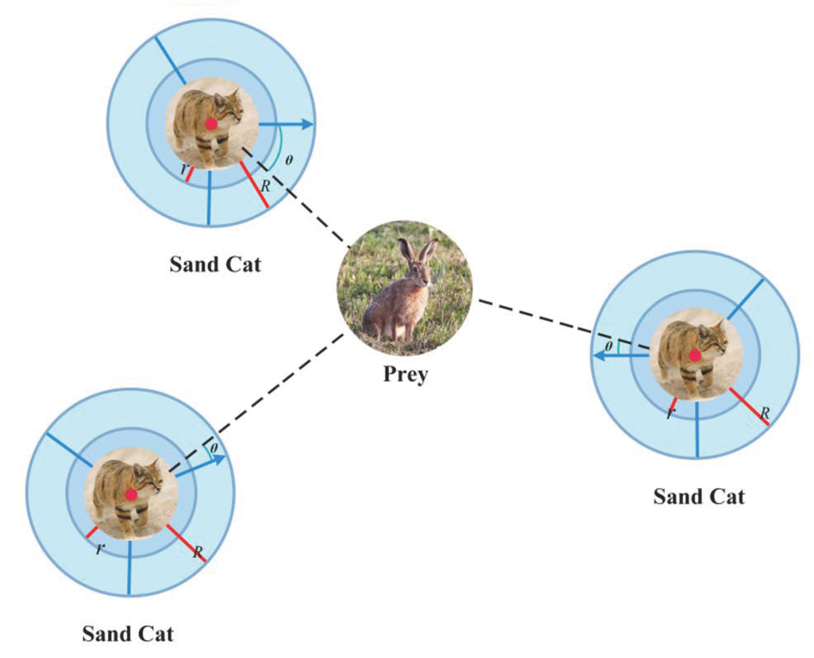
2.1.2. Search for Prey (Detect)

Sand cats have a distinctive ear canal structure that allows them to detect low-frequency noise. This ability helps them assess noise conditions, aiding in their search for prey and facilitating the transition between searching and attacking phases. Equations (4)–(6) present the mathematical model for how sand cats perceive low-frequency noise.
r G = s M ( 1 t / i t e r max )
r = r G × r a n d
R = 2 × r G × r a n d r G
The sand cat’s ability to search for prey depends on noise frequencies ranging from 0 to 2 kHz; therefore, the sand cat’s auditory sensitivity vector R G ranges between 0 and 2 and shows a linear declining trend. The maximum sensitivity S M of a sand cat is 2; i t e r max represents the maximum number of iterations; r is the auditory sensitivity range vector for each sand cat; R is the coefficient vector for balancing attack and search strategies; rand is a random number between 0 and 1; t represents the current iteration number.

2.1.3. Hunting for Prey (Development)

During the search process, the sand cat adjusts its position based on the distance to the best location and its sensitivity range. By incorporating a random angle θ, the sand cat can explore in different directions, increasing the level of randomness during exploration. This exploration strategy enhances the algorithm’s capability to discover new local optima within the search area. Additionally, the algorithm guarantees that each updated sand cat position lies between its current location and the prey. The mathematical representation of the prey attack phase is described by Equations (7) and (8).
D = r a n d × X b ( t ) X ( t )
X ( t + 1 ) = X b ( t ) D × cos ( θ ) × r
where D represents the distance vector between the best individual’s position and the current individual’s position; X b represents the position vector of the current best individual; X represents the position vector of the current individual. X t + 1 represents the position vector of the updated individual. Figure 2 shows the sand cat approaching the hunting location and attacking the prey using a random angle θ.

2.1.4. Search and Attack Choice

Figure 3 represents the position update diagram. According to sand cat hunting behavior, its updated location mode is divided into two types: searching for prey or attacking prey. The choice between these two methods is determined by the balancing parameter R. When R 1 , the sand cat attacks the prey; when R > 1, the sand cat needs to search for the next prey. This is depicted in Equation (9).
X ( t + 1 ) = X b ( t ) D × cos ( θ ) × r ,   R 1 ; r × X b c ( t ) r a n d × X ( t ) ,   R > 1 ;
where X b represents the current best position vector; θ is randomly assigned to each cat’s position update in order to ensure that it takes on values within a certain range, as it is used in the cosine value, which ensures that it will be closer to the hunting area based on the results; X b c represents the current best candidate’s position vector.

2.2. Multi-Strategy Improved Sand Cat Swarm Optimization Algorithm (MISCSO)

2.2.1. Multi-Population Strategy

During feeding, sand cat swarm behavior tends to homogenize the population towards prey locations, limiting global search mobility and potentially trapping the algorithm in local optima. To address this, a multi-population strategy is proposed in this study. The algorithm divides the population into three subpopulations—exploitation, balance, and exploration—based on fitness levels, enhancing population diversity and aiding in escaping local optima. Each subpopulation undergoes separate update strategies during optimization, followed by collective evaluation and re-division into new subpopulations. The mathematical model is represented by Equation (10) in the paper [30,31]:
p o p u l a t i o n   s i z e = 0.3 × N P , Exploitation   subpopulation 0.4 × N P , Balance   subpopulation 0.3 0.3 × ( t t max ) × N P , Exploration   subpopulation
Here, NP represents the number of populations. In order to avoid premature convergence, the size of the exploitation subpopulation should not be too large, set as 0.3 NP. At the same time, to ensure the efficiency of convergence in the later stages of the algorithm, as optimization progresses, populations with low fitness will be eliminated, and the exploration subpopulation will gradually decrease. The specific division of populations is calculated as Equations (11) and (12):
P i = ( N P r a n k ( f ( X i ) ) + 1 ) / N P
X i = Exploitation   subpopulation , i f   P i > 0.7 Balance   subpopulation , i f   P i > 0.3 0.3 × ( t t max )   P i 0.7 Exploration   subpopulation , i f   P i 0.3 0.3 × ( t t max )
Specifically, the exploitation subpopulation utilizes information from the dominant individuals for local exploitation and the provision of better solutions. The balance subpopulation simultaneously performs exploitation and exploration behaviors. The exploration subpopulation explores more of the problem space and maintains population diversity. Population diversity is a guarantee of the algorithm’s exploration capability, and using a multi-population strategy enhances the algorithm’s global search capabilities while also avoiding premature convergence and falling into the trap of local optima [32].

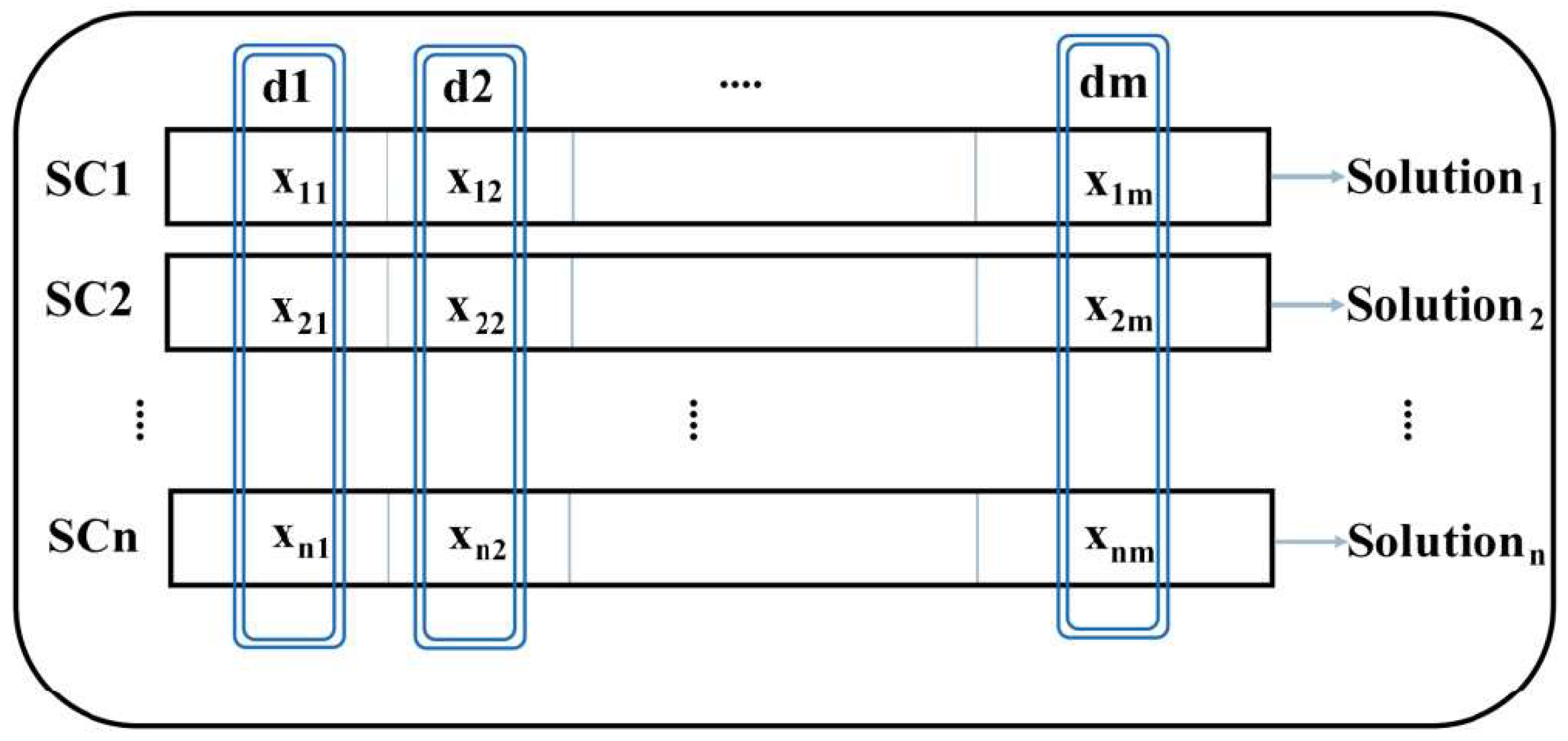
2.2.2. Distribution Estimation Learning Strategy

Balancing exploration and exploitation has always been the focus of swarm intelligence algorithms. When the development capability exceeds the exploration capability, the algorithm may fall into local optima or even stagnation; conversely, it may lead to a slow convergence speed. Therefore, while enhancing algorithm performance, it is necessary to find a balance between development and exploration [33]. This paper introduces a distribution estimation learning strategy, using probability models to represent relationships between individuals and boost algorithm performance. By fully utilizing the information from advantageous populations, the algorithm improves its exploration capability and enhances its development potential, striking a balance between exploration and exploitation.
The distribution estimation learning strategy utilizes the current dominant population to compute a probability distribution model and sample new individuals based on this probability distribution model [34]. This paper adopts the weighted maximum likelihood estimation method to estimate the distribution model. The mathematical model of this strategy is described as Equations (13)–(15):
x m e a n = i = 1 N P 2 ω i × x i
ω i = ln ( N P / 2 + 0.5 ) ln ( i ) i = 1 N P / 2 ( ln ( N P / 2 + 0.5 ) ln ( i ) )
C o v ( i ) = 1 N P / 2 i = 1 N P / 2 ( x i x m e a n ) ( x i x m e a n ) T
In the equation, x m e a n represents the weighted average of the dominant population and ω i represents the weighted coefficients of the dominant population. These coefficients are arranged in descending order according to their fitness levels. C o v represents the weighted covariance matrix of the dominant population.
For the developing population, the evolutionary direction of the sand dune cats’ individuals is modified using information from the dominant population to enhance the algorithm’s development and optimization performance. The updating method for advantageous population locations is expressed as Equation (16):
x i t + 1 = G a u s s i a n ( x m e a n , C o v ( i ) ) + r a n d n × ( x m e a n x i t )
For the exploring population, since they are far from the optimal solution, the mean point should be far from the suboptimal solution. This can drive the sampling points closer to the optimal solution, thereby enhancing the algorithm’s exploratory capabilities. The update formula for the exploring population’s positions is described as Equation (17):
x i t + 1 = G a u s s i a n ( x m e a n , C o v ( i ) ) + r a n d n × ( x m e a n x i t )
In general, the probability distribution model selects some dominant individuals from the current population for evaluation in each iteration, and then samples to generate a new population based on the constructed Gaussian probability distribution model, which serves as the sample for the next distribution model. The distribution estimation learning strategy effectively balances exploration and exploitation while enhancing the algorithm’s performance [35].

2.2.3. Elite Pool Strategy

In the SCSO algorithm, the attack prey phase is crucial for effective performance. Formulas (16) and (17) show that individual updates rely heavily on the involvement of the best individuals in the colony. This participation brings individuals closer to the optimal solution and accelerates convergence [36]. When the best individual gets trapped in a local optimum, it affects the entire population’s quality, leading to local optima and reduced accuracy [37]. To address this, an elite pool strategy is proposed. This strategy selects the top three individuals with high fitness values and the average of the dominant population, storing them as candidates in Equation (18).
x e p = { x e p 1 , x e p 2 , x e p 3 , x m e a n }
In the search process, the attack prey phase involves randomly selecting the best individual from the elite pool to replace [38]. Each of the four candidate solutions has an equal selection probability of 0.25. The variety of candidate solutions in the elite pool not only broadens the search space but also improves the algorithm’s capacity to avoid local solutions.

2.2.4. Cauchy Perturbation Strategy

The Cauchy distribution’s distinctive features include long tails on both ends and a pronounced peak at the central origin. By utilizing the Cauchy operator as a disruptive step, the optimal individual increases the chances of moving to a more advantageous position. After reaching a local optimal solution, the Cauchy operator adjusts the step length, expanding it to facilitate the algorithm’s departure from the position of the local optima [39].
Conversely, when the individual is being precisely developed, the operator decreases the step length, accelerating the convergence speed. The specific disturbance method is expressed as Equation (19):
x n e w b ( j ) = x b ( j ) + c a t h y × x b ( j )
X b represents the individual with the current optimal fitness; X n e w b represents the optimal individual after undergoing Cauchy mutation. Combined with the disturbance probability, the update method for the current global optimal position is calculated as Equation (20):
x b ( j ) = x n e w b ( j ) ,   i f   f ( x n e w b ) < f ( x b ) x b ( j ) ,   i f   f ( x n e w b ) f ( x b )
The use of the Cauchy disturbance strategy enhances the disturbance ability of the Cauchy operator, improving the algorithm’s global optimization speed and convergence speed while also strengthening the algorithm’s convergence accuracy [40].

2.2.5. Time Complexity

The time complexity of an algorithm indicates the amount of processing required by the algorithm as the problem size increases. In the case of SCSO with a population size of N, a problem dimension of D, and a maximum iteration count of T, the time complexity can be viewed in terms of population initialization and individual position updates. The fitness calculation during initialization has a time complexity of O (N × D). Each individual’s position is updated over T iterations, resulting in a time complexity of O (T × N × D) for the individual position update process. Simplifying and removing lower-order terms, the overall time complexity of SCSO can be represented as O (T × N × D).
For the MISCSO algorithm, the time complexity is as follows:
(1)
The initialization parameter has a time complexity of O (1).
(2)
The initialization of population positions has a time complexity of O (N × D).
(3)
Sand cat predation has a time complexity of O (T × N × D).
(4)
The position update based on the distribution estimation learning strategy has a time complexity of O (T × N × D).
(5)
The cost of function computation includes the algorithm computation time O (T × N × C), elite pool strategy calculation time O (T × N × C), and distribution estimation learning strategy calculation time O (T × N × C), summing up to O (3 × T × N × C).
In summary, the total time complexity of the MISCSO algorithm is: O (MISCSO) = O (1 + N × D + 4 × T × N × C + 2 × T × N × D). Due to 1 << T × N × C, 1 < T × N × dim, N × dim < T × N × C, and N × dim < T × N × dim, it can be simplified as O (MISCSO) = O (3 × T × N × C + 2 × T × N × D).

2.3. Mathematical Model for UAV Path Planning
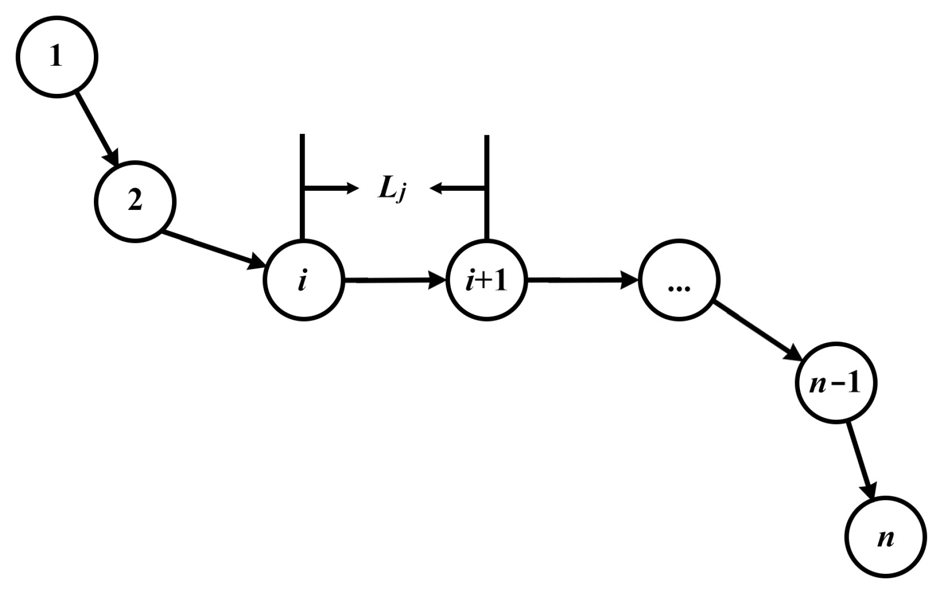
When a UAV is executing a flight mission, it is subject to various constraints, including three-dimensional environmental space constraints and its own performance limitations. Therefore, before planning the path of a UAV, a cost constraint function must be established based on the relevant constraints. The rationality of establishing the flight cost constraint function directly affects the success or failure of the UAV flight mission. If the cost constraint function is established irrationally, it is highly likely to result in a longer path, insufficient fuel, and ultimately mission failure. Based on the UAV flight environment and the UAV’s performance characteristics, this paper establishes a three-dimensional path-planning mathematical model based on path cost, threat cost, altitude cost, and smoothness cost.

2.3.1. Path Cost

During the flight of a UAV, its maximum flight distance is influenced by its structure and energy. In order to ensure safety and normal flight, due to hardware structure issues, the UAV must fly in a straight line for a certain distance in order to change its heading. This condition not only avoids frequent turns and changes of direction but also reduces the occurrence of accidents. Therefore, in order to achieve safe flight, the UAV’s path planning needs to be carried out under certain conditions. Figure 4 depicts the flight path of the UAV. The formula for the path cost function is dictated by Equation (21):
F 1 J i = j = 1 n 1 P i j P i j + 1
where Ji represents the flight path of the UAV, consisting of a set of n path nodes P i j = x i j , y i j , z i j ; i indicates the i-th UAV; j indicates the j-th node of the flight path of this UAV; P i j P i j + 1 denotes the straight-line distance between two adjacent nodes.

2.3.2. Threat Cost

Threat cost refers to the level of threat posed to UAV flight by threatening obstacles in the environment. The closer the UAV is to the threatening source in the environment, the higher the threat coefficient, making it more likely to cause safety issues. In the modeling process, the threat area is often simplified to a circular shape, which can greatly simplify the calculation process of flight path planning. Let E be the set of all obstacles with threats; the obstacle model is a cylinder, with its projection center at Ce; Re is the obstacle radius; D is the UAV diameter. S represents the danger zone of the obstacle, which depends on the UAV’s positioning accuracy and the flight environment. There is a danger zone around the threat object, where collisions are likely to occur. The diameter of the danger zone is R + S. By considering D and S, the threat cost function is calculated using the following Equation (22):
F 2 ( W i ) = j = 1 n 1 e = 1 e T e ( P i , j P i , j + 1 ) T e ( P i , j P i , j + 1 ) = 0 ,   i f   d e > S + D + R e ( S + D + R e ) d h , i f   D + R e < d e S + D + R e ,         i f   d e D + R e
D is determined by the size of the UAV, and S is determined by various factors. If the UAV is flying in a relatively safe environment, S is only tens of meters; if the UAV is flying in harsh conditions with poor signal, S may be several hundred meters. When the UAV is flying in a threat area, the threat cost is 0; when the UAV passes through a danger zone, the closer it is to the center Ce, the greater the threat cost; when the UAV passes through a collision zone or collides with a threat obstacle, the UAV will crash, and the threat cost is infinity.

2.3.3. Altitude Cost

A reasonable flight altitude can save fuel and ensure the safety of the UAV. Usually, in order to ensure concealment during flight, the UAV often cannot fluctuate too much in height and needs to maintain stable low-altitude flight. In addition, in order not to threaten the safety of other manned aircraft and due to battery endurance, it is necessary to restrict the flight altitude of the UAV. The maximum flight altitude is defined as hmax, the minimum altitude is defined as hmin, and for each path point Pi,j, the cost of altitude hi,j can be calculated using the following Equation (23):
H i , j = h i , j ( h max + h min ) 2 ,   i f   h min h i , j h max ; ,   o t h e r w i s e .
In the equation, hi,j represents the flight altitude of the path point with the ground as the reference surface. For path points that do not fall within the specified height range, the cost of altitude is considered as infinite. By summing up the altitude costs for all path points Hi,j, the overall height cost of the path can be calculated using the following equation:
F 3 ( J i ) = j = 1 n H i , j

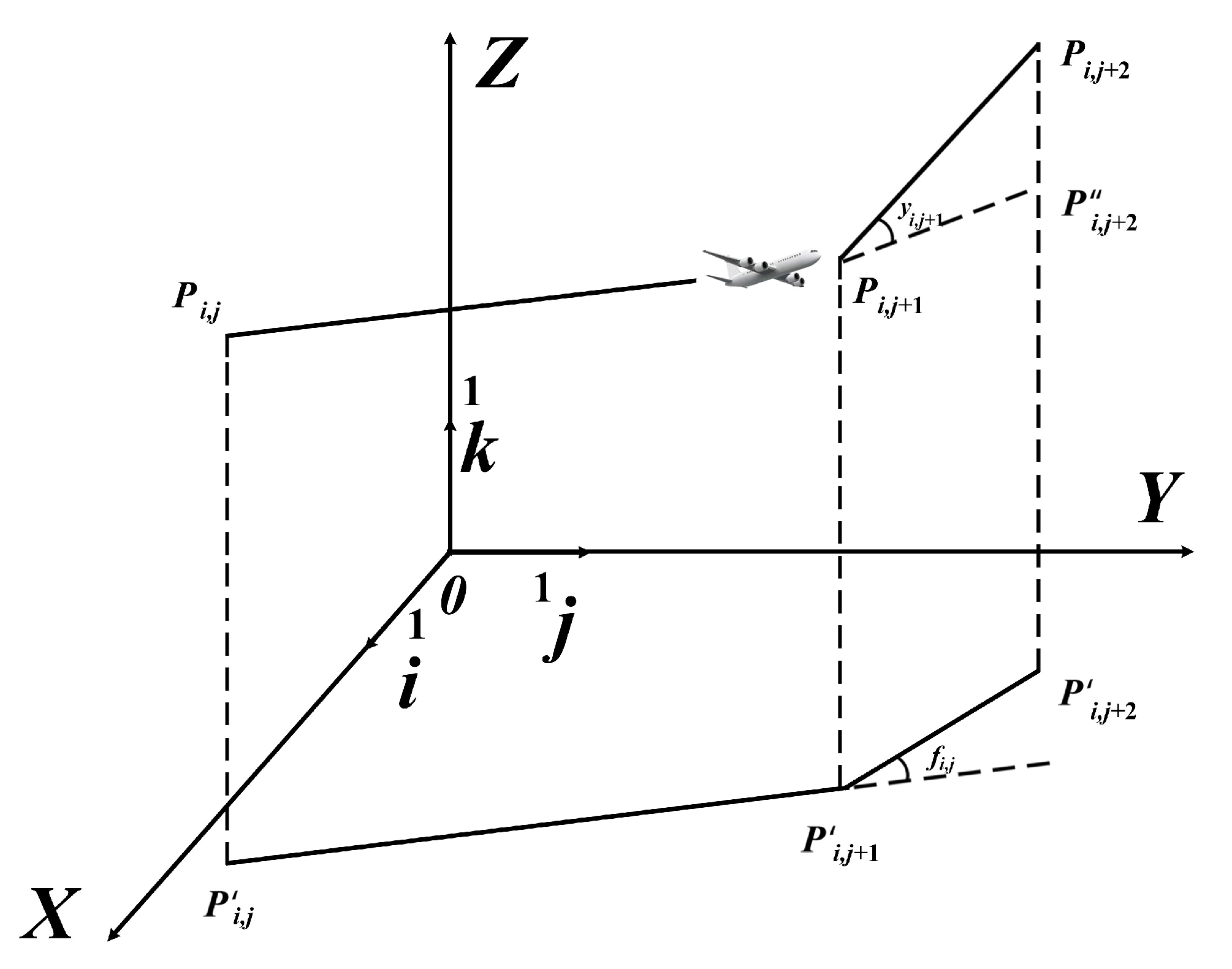
2.3.4. Smoothness Cost

During the flight, it is also necessary to consider the stability of the UAV’s flight path. Otherwise, excessive fluctuations can increase the probability of risk. Stability is mainly related to the yaw angle and pitch angle. The calculation of the yaw angle and pitch angle is shown in Figure 5 [41].
Where P i , j P i , j + 1 and P i , j + 1 P i , j + 2 are the projections of two adjacent path segments on the OXY plane, with k being a unit vector in the Z direction; yaw angle φ i , j is the angle between the projections of the two segments; pitch angle ψ i , j is the angle between the projection vectors of path segments P i , j P i , j + 1 and P i , j + 1 P i , j + 2 . c1 and c2 are the penalty coefficients for yaw angle and pitch angle, respectively. The projection vector, yaw angle, pitch angle, and stability cost can be expressed by the following Equations (25)–(28):
P i , j P i , j + 1 = k × ( P i , j P i , j + 1 × k )
φ i , j = a r c t a n P i , j P i , j + 1 × P i , j + 1 P i , j + 2 P i , j P i , j + 1 × P i , j + 1 P i , j + 2
ψ i , j = a r c t a n z i , j + 1 z i , j P i , j P i , j + 1
F 4 ( J i ) = c 1 j = 1 n 2 φ i , j + c 2 j = 1 n 1 ψ i , j ψ i , j 1

2.3.5. Total Cost

Based on the cost path, threat cost, altitude cost, and smoothness cost of path Ji, the total cost function of three-dimensional drone path planning can be defined as Equation (29):
F ( J i ) = k = 1 4 b k F k ( J i )
where bk represents the weight coefficient.

3. Results and Discussion

In order to maintain the rigor and impartiality of the experiments, all simulation tests in this research were carried out under identical experimental conditions using MATLAB R2023a as the simulation platform. This standardized approach ensured consistency and comparability in the evaluation of results across different experimental runs. The operating system used was Microsoft Win 11 (64-bit), and the processor was AMD Ryzen 5 4600U with Radeon Graphics @2.10 GHz. The system had 16 GB of memory. The basic parameter settings for the experiments are as follows: population size Pop = 300, dimension d = 100, and maximum number of iterations M = 150.

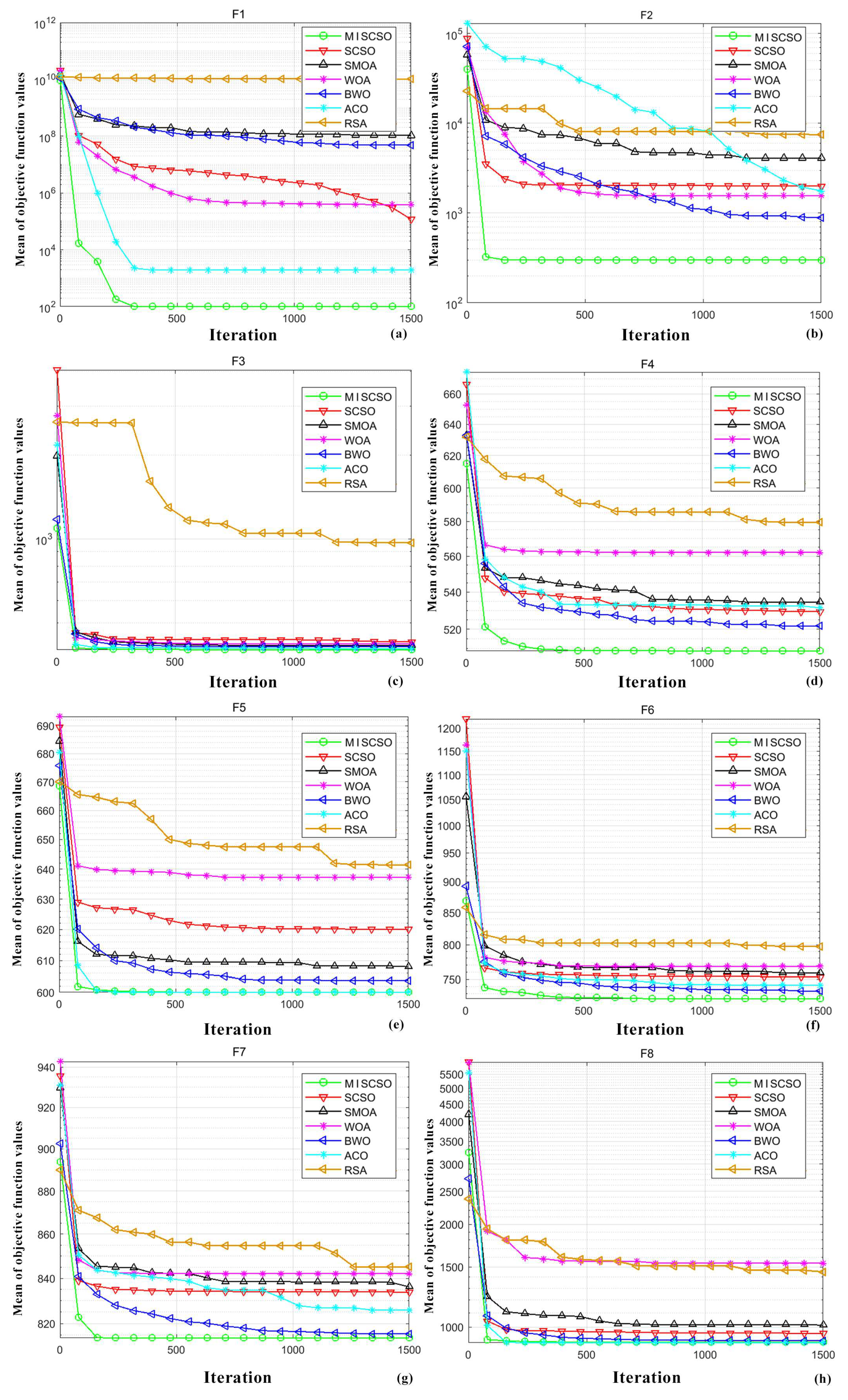
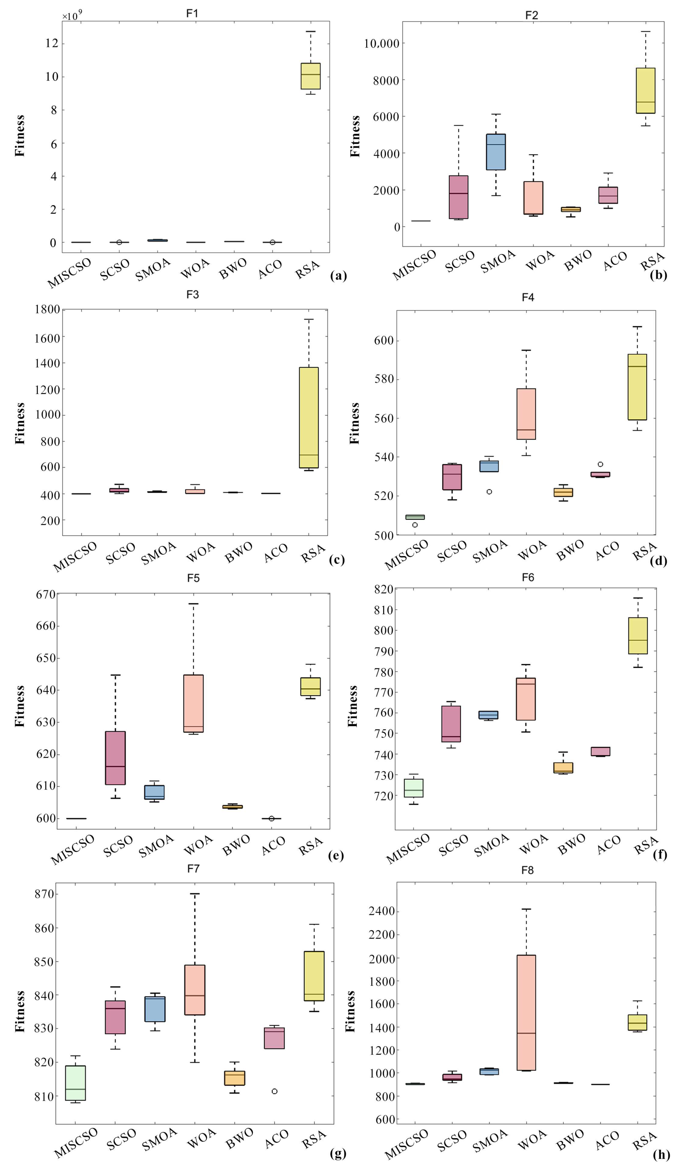
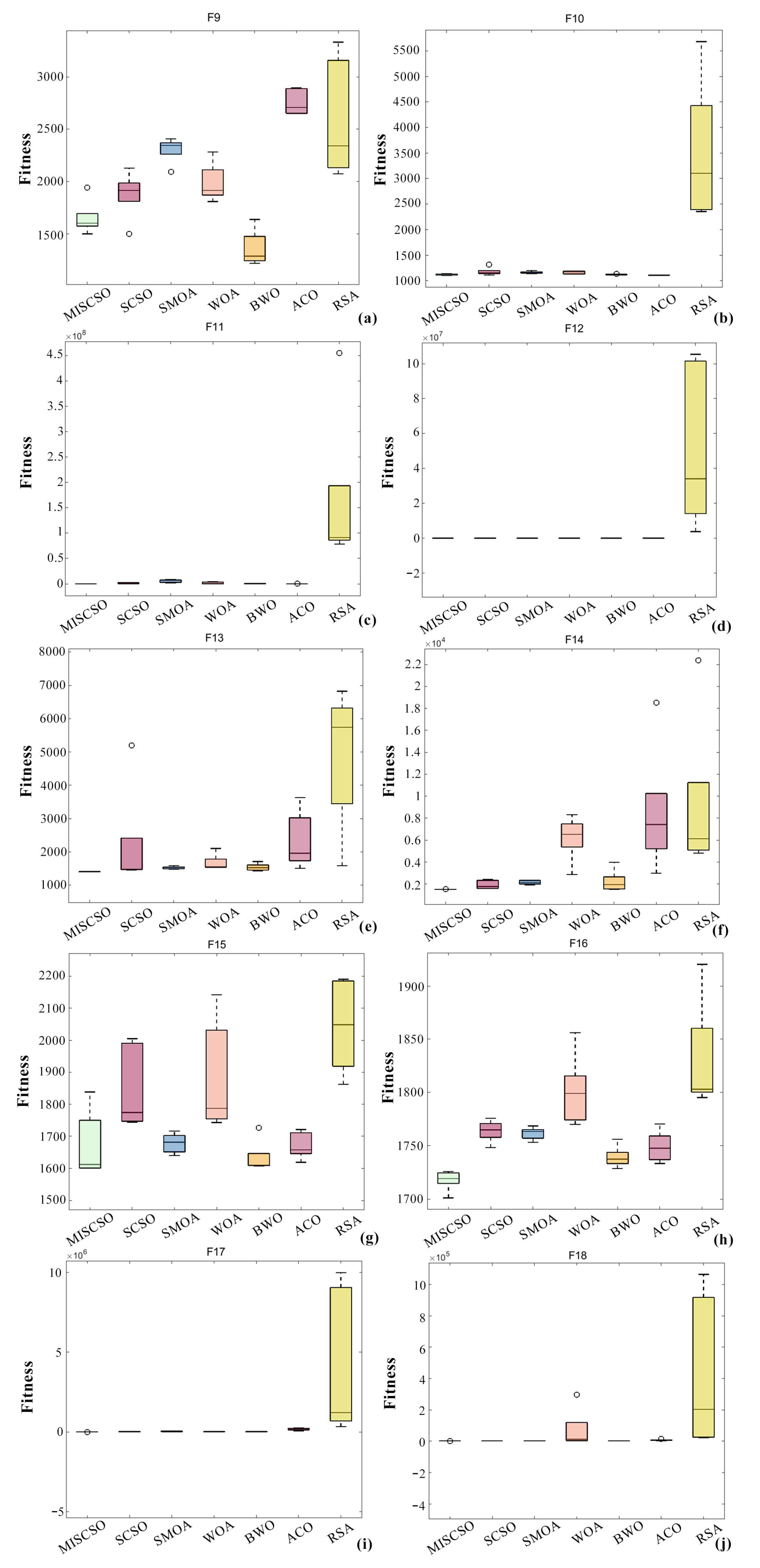
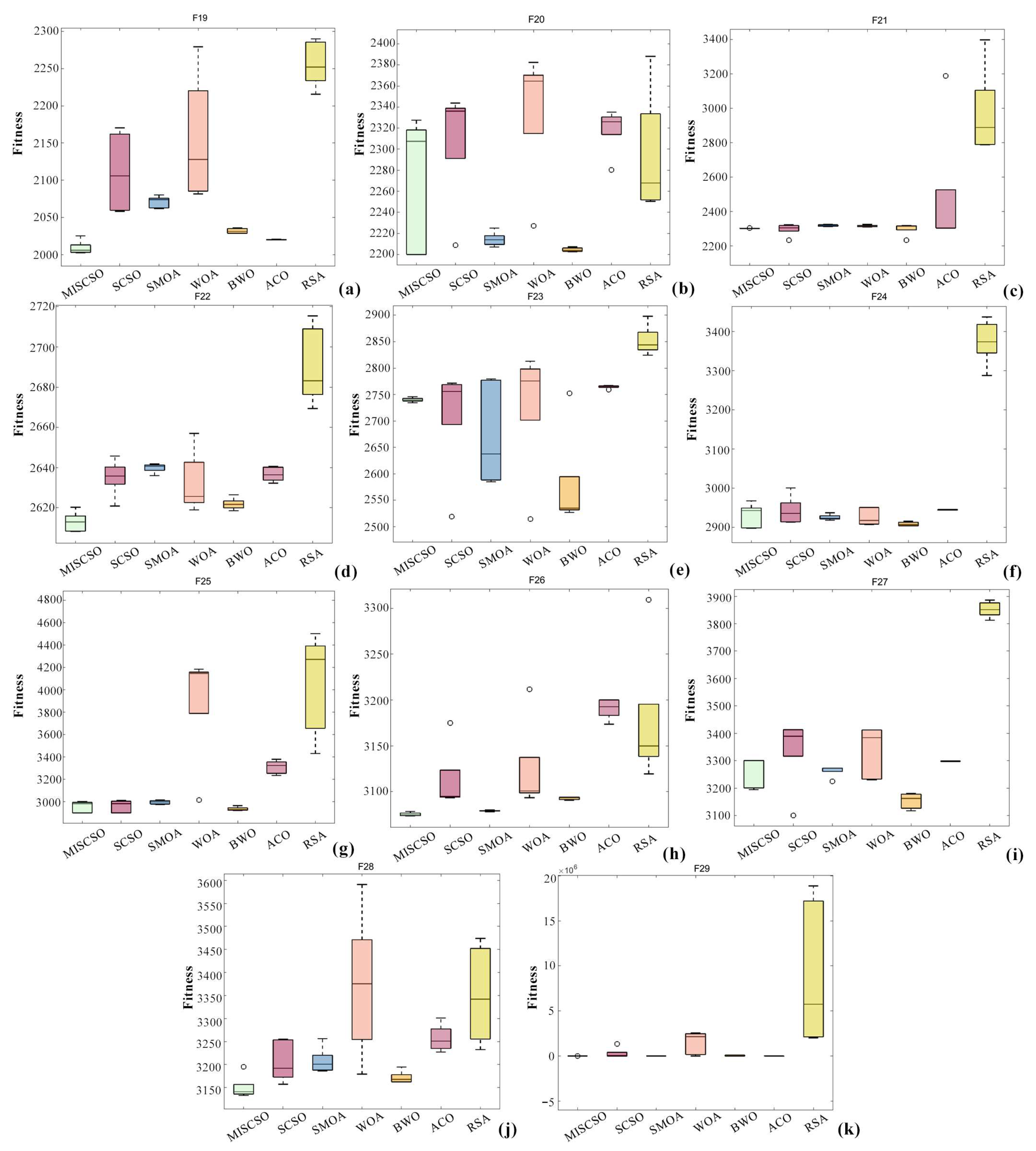
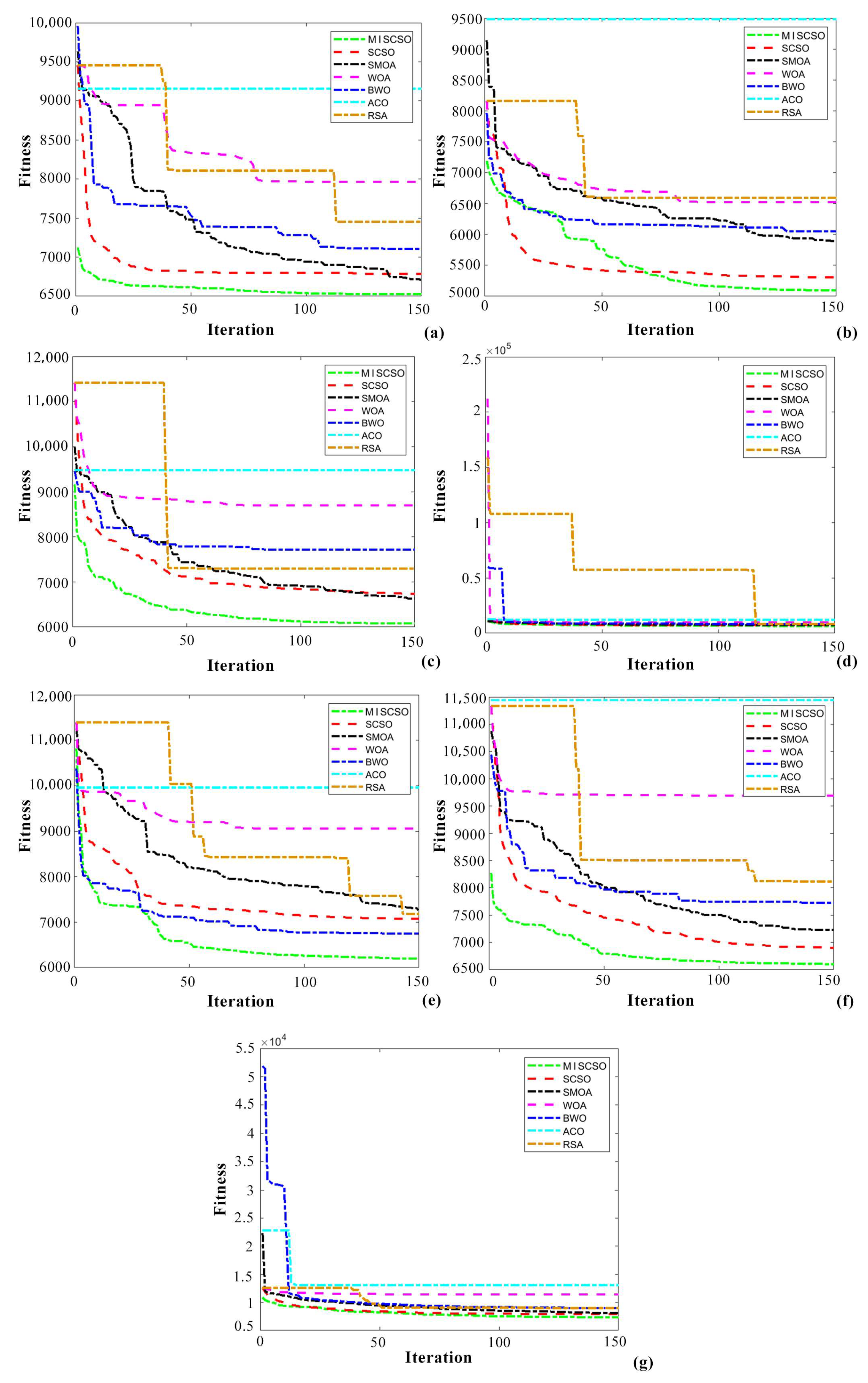
3.1. MISCSO Algorithm Evaluation

To evaluate the performance of MISCSO in handling complex functions, this study compared MISCSO with several other optimization algorithms, including SCSO, Spider Monkey Optimization algorithm (SMOA), Whale Optimization Algorithm (WOA), Beluga whale optimization (BWO) algorithm, Ant Colony Optimization (ACO), and Reptile Search Algorithm (RSA), using the CEC2017 complex functions. Table 1 provides detailed information on the CEC2017 functions, which consist of a variety of challenging problems, such as rotated traps, that test the optimization capabilities of the algorithms. The functions are categorized as unimodal, simple multimodal, hybrid, and composition functions.
For the unimodal functions f1 and f2 (Figure 6), only the MISCSO algorithm found the global optimum, while the solutions found by the other algorithms were of low quality and even stuck in local optima. For the multimodal functions f3 to f9, the MISCSO algorithm had the best fitness values in Figure 6c–e,h, with fast convergence speed. Although the fitness value was lower than BWO’s in Figure 7a, the BWO algorithm stagnated in later iterations and converged more slowly than the MISCSO algorithm. The RSA algorithm exhibited a stair-like iteration trend in Figure 6c–e and Figure 7a, but still fell into local optima, with worse fitness values than the MISCSO algorithm. For the hybrid modal functions f10 to f19, in Figure 7b, except for the RSA algorithm, all other algorithms found the optimal solution. However, the MISCSO algorithm had the lowest fitness value in the early iterations, indicating a higher quality of path planning. In Figure 7c,d,i, the fitness values of the MISCSO algorithm were significantly better than other algorithms. In Figure 7e,f,h,j and Figure 8a, the fitness values of the seven algorithms were similar, but the MISCSO algorithm had a faster convergence speed. In Figure 7g, although the fitness value of BWO was better than the MISCSO algorithm, its convergence speed and algorithm stability were worse than the MISCSO algorithm. For composition functions f20 to f29, in Figure 8c,f, all algorithms except for the RSA algorithm found relatively good solutions. In Figure 8d,g,h,j,k, the MISCSO algorithm had the best fitness values and a faster convergence speed. In Figure 8b,e,i, the BWO algorithm had the best fitness values, but the MISCSO algorithm exhibited a faster convergence speed. Additionally, in Figure 8k, the BWO algorithm got stuck in a local optimum.
Table A1 shows the best value, standard deviation, average value, and worst value of the fitness values for the seven algorithms under unimodal functions. In function f1, except for the ACO and MISCSO algorithms, whose best values approach a fitness value of 100, the rest of the functions deviate too greatly. Additionally, the standard deviation of the MISCSO algorithm is 105 lower than that of the other algorithms. In function f2, the fitness value of the MISCSO algorithm directly reaches 300 with a standard deviation of 0. The best value of the SCSO algorithm approaches 300, but the other values have significant errors. The BWO algorithm performs slightly worse than the SCSO algorithm in terms of its best value but is second to the MISCSO algorithm in the remaining values. Table A2 shows the best value, standard deviation, average value, and worst value of the seven algorithms under multi-modal functions. In function f3, the fitness value of the MISCSO algorithm equals the function fitness value with a standard deviation of 0. The ACO algorithm outperforms the other five algorithms in standard deviation, average value, and worst value, but the SCSO algorithm surpasses the ACO algorithm in its best value. In function f4, the fitness values of each algorithm are similar, but the MISCSO algorithm still remains the best in all four values. In function f5, the fitness value of the ACO algorithm reaches 600 with a standard deviation of 0. The MISCSO algorithm is almost as good as the ACO algorithm, falling only slightly behind. The SMOA and BWO algorithms perform similarly, and both outperform the SCSO, WOA, and RSA algorithms. Although the MISCSO algorithm does not have the optimal standard deviation in functions f6 and f7, the rest of the values are still optimal. In function f8, the ACO algorithm has the best fitness value, equal to the function’s fitness value. Among the other algorithms, although the BWO algorithm has the lowest standard deviation, the MISCSO algorithm’s average and worst values are optimal, and the best value is the same as ACO, reaching 900. Table A3 shows the best value, standard deviation, average value, and worst value of the seven algorithms under multimodal functions. In function f10, except for RSA which has a large deviation, the ACO algorithm is optimal in standard deviation, average value, and worst value, but the MISCSO algorithm is optimal in the best value. In functions f11~f14 and f17, all algorithms except MISCSO have significant deviations from the function fitness value, demonstrating that the MISCSO algorithm maintains strong performance in complex situations. In function f15, although the SMOA algorithm is superior in standard deviation and worst value, the MISCSO algorithm excels in the best value compared to SMOA. In function f16, the algorithms have small differences from the function fitness value, with the MISCSO algorithm being optimal in the best value, average value, and worst value. In function f19, although the ACO algorithm has the smallest standard deviation, the MISCSO algorithm is optimal in the remaining values and closest to the function fitness value. Table A4 shows the best value, standard deviation, average value, and worst value of the seven algorithms under multi-modal functions. In function f20, although the BWO algorithm has the optimal standard deviation, average value, and worst value, the MISCSO algorithm’s best value is superior to BWO, with the SMOA algorithm showing relatively better standard deviation, while the other algorithms have similar values. In function f21, the MISCSO algorithm excels in standard deviation, worst value, and best value compared to the other algorithms, with ACO and RSA having high standard deviations and showing instability. In function f22, the SMOA algorithm has the lowest standard deviation, but the MISCSO algorithm excels in best value, average value, and worst value, with the remaining algorithms having smaller differences. In function f23, SCSO, SMOA, WOA, and BWO show significant fluctuations compared to the other algorithms, with high standard deviation values, while the MISCSO and ACO algorithms are more stable, with the MISCSO algorithm having the best fitness value. In function f24, the BWO and ACO algorithms have similar values and stability, but their fitness values are lower compared to MISCSO, and the RSA algorithm deviates the most from the fitness value. In function f25, the MISCSO algorithm has the best fitness value, matching the function’s fitness value, followed by the SCSO algorithm, and the SMOA and BWO algorithms excel over WOA, ACO, and RSA. In function f26, the values of the MISCSO and SMOA algorithms are close, with the MISCSO algorithm superior to SMOA in all aspects except for standard deviation, and the other algorithms, although inferior to MISCSO, have small differences in values. In function f27, the SCSO algorithm has the best value closest to the function’s fitness value, but with the highest standard deviation. The BWO algorithm excels in all values except for standard deviation, with the MISCSO algorithm’s best value second only to BWO. In function f28, except for standard deviation, the MISCSO algorithm has the best values, while the WOA and RSA algorithms have significantly higher standard deviations than the other algorithms, with small differences in the remaining algorithms. In function f29, the fluctuations increase for all algorithms, resulting in larger deviations from the function’s fitness value, with the RSA algorithm even reaching a deviation magnitude of 104. However, the MISCSO algorithm still achieves better fitness values with minimal deviations.
According to the above analysis, MISCSO exhibits a faster convergence speed in the optimization process of benchmark functions and can promptly escape local extreme situations, thereby improving the precision of optimization. In terms of fitness values, the deviation is almost zero in unimodal functions, and the fitness values are closest to the function’s fitness values among the seven algorithms, indicating that the MISCSO algorithm can accurately find the optimal solution. In multimodal functions, MISCSO achieves the best values equal to the function’s fitness values in f3 and f8, with values superior to other functions. Although the ACO algorithm has the best fitness values in f5 and f8, it is outperformed by the MISCSO algorithm in other multi-modal functions, especially with the worst fitness values in f9. In hybrid functions f11, f12, f17, and f18, apart from the MISCSO algorithm, the values of the other algorithms deviate significantly from the function’s fitness values, and the fluctuation magnitude of the algorithms increases, proving that the MISCSO algorithm can maintain good stability and optimization capability even in complex environments. In composition functions, the MISCSO algorithm has a relatively high standard deviation, but the differences from the lowest standard deviation are small, with values of the seven algorithms being fairly close. However, the MISCSO algorithm has the best fitness values, and in f29, noticeable fluctuations are observed in all algorithms except for MISCSO, with most algorithms deviating from the function’s fitness values by magnitudes reaching 102 and higher. In conclusion, it is evident that the improved MISCSO algorithm proposed in this study is an effective algorithm for planning flight paths.
In order to analyze the distribution characteristics of the improved algorithms, box plots were constructed based on the independently solved results of each algorithm on 29 test functions. For unimodal functions f1 and f2, in Figure 9a, the fitness values of all algorithms are similar except for the RSA algorithm, with the SCSO and ACO algorithms displaying outliers. In Figure 9b, MISCSO, BWO, and ACO have minimal deviations, with MISCSO having the smallest median and highest fitness value. For multimodal functions f3 to f9, the MISCSO algorithm only exhibits outliers in Figure 9d and Figure 10a, with the lowest median value. In Figure 9g, although the MISCSO algorithm has significant deviations, it has the lowest median value. For hybrid functions f10 to f19, except for the RSA algorithm in Figure 9b–d, the median values and dispersion of the other algorithms do not differ significantly. In Figure 10g, although the MISCSO algorithm has a large dispersion, it still has the lowest median value and no outliers. For composition functions f20 to f29, in Figure 11c,d,g,h, the MISCSO algorithm demonstrates superior stability and fitness values. In Figure 11b, the MISCSO algorithm shows a large deviation but no outliers.
In general, on the convergence plots of the test functions, it can be concluded that the MISCSO algorithm converges faster and achieves higher solution accuracy compared to the original algorithm. In unimodal functions, it can accurately and quickly find the optimal value, demonstrating its strong search capability. In multimodal functions, it can escape local optimal values, indicating that the improved strategy effectively increases the diversity of the population. In hybrid functions and composition functions, it can still find the optimal value quickly, showcasing its potential in solving complex real-world problems. Additionally, in the box plots, it is observed that the MISCSO algorithm exhibits better robustness, with smaller median values and dispersion. The probability of outliers occurring is also smaller, proving the strong stability and high fitness of the MISCSO algorithm.

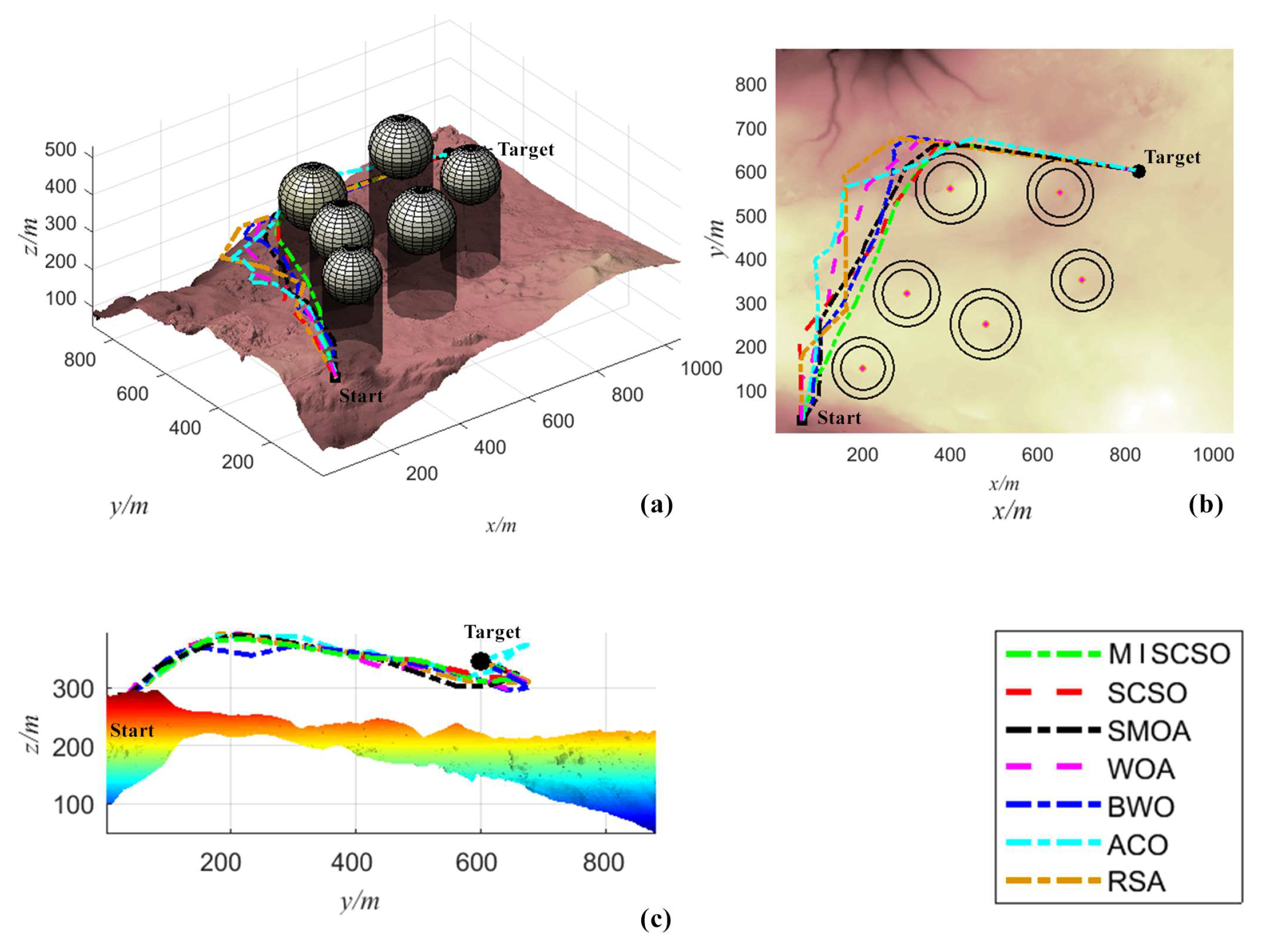
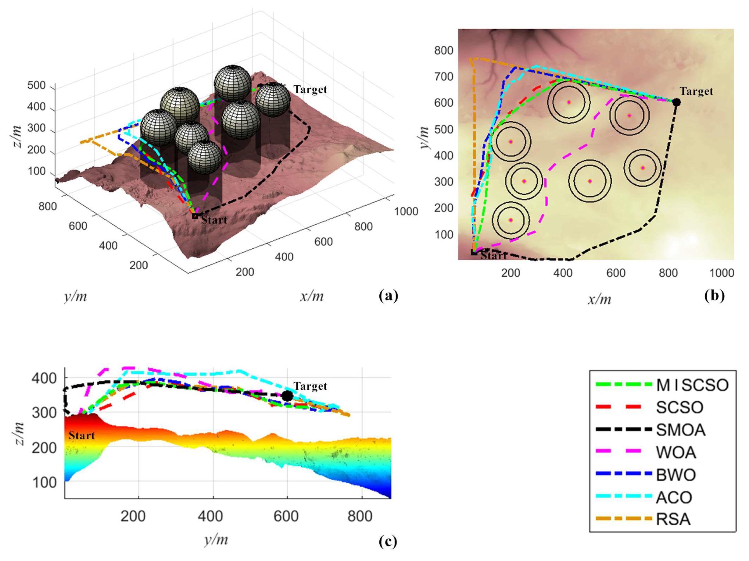
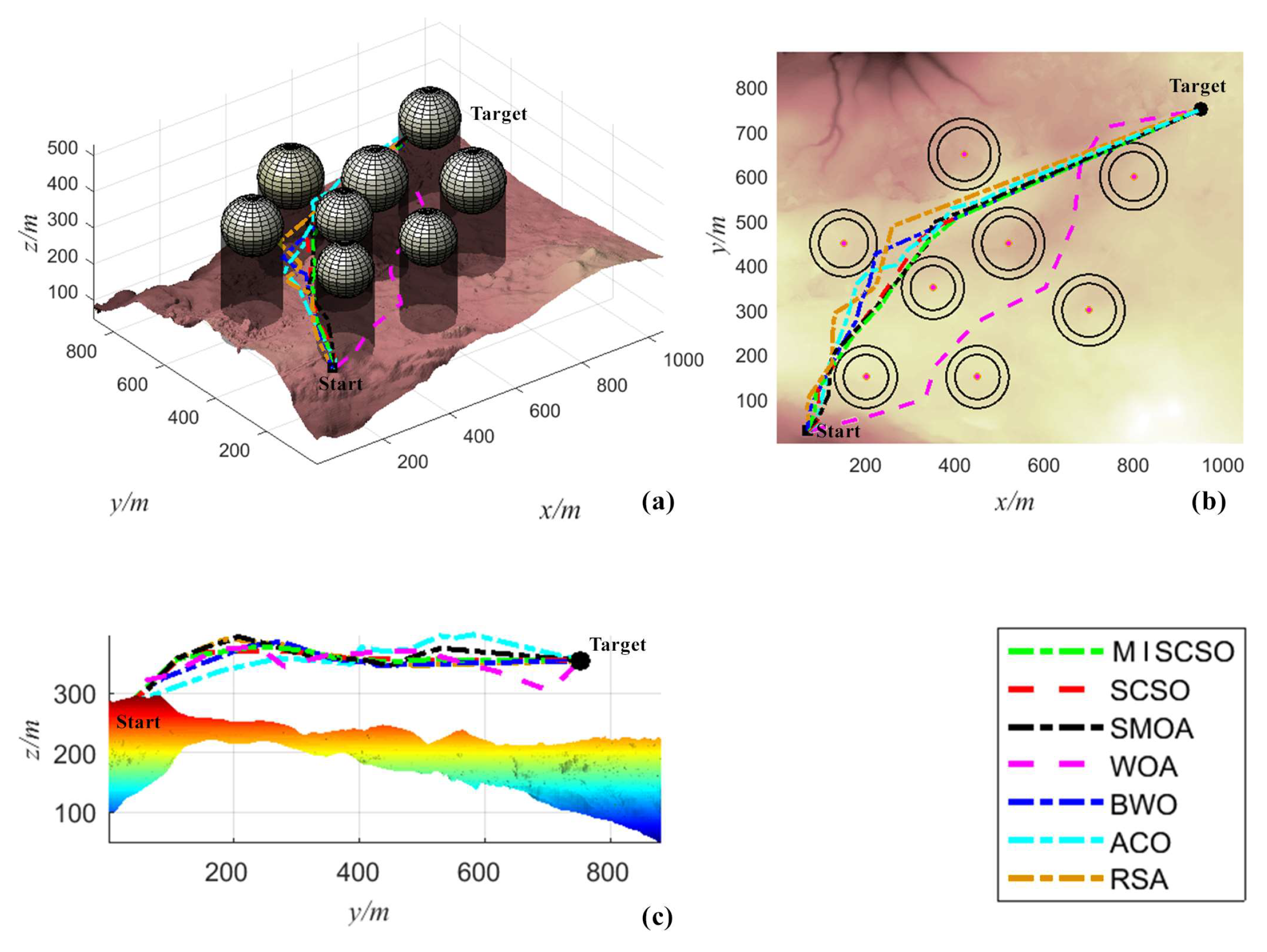
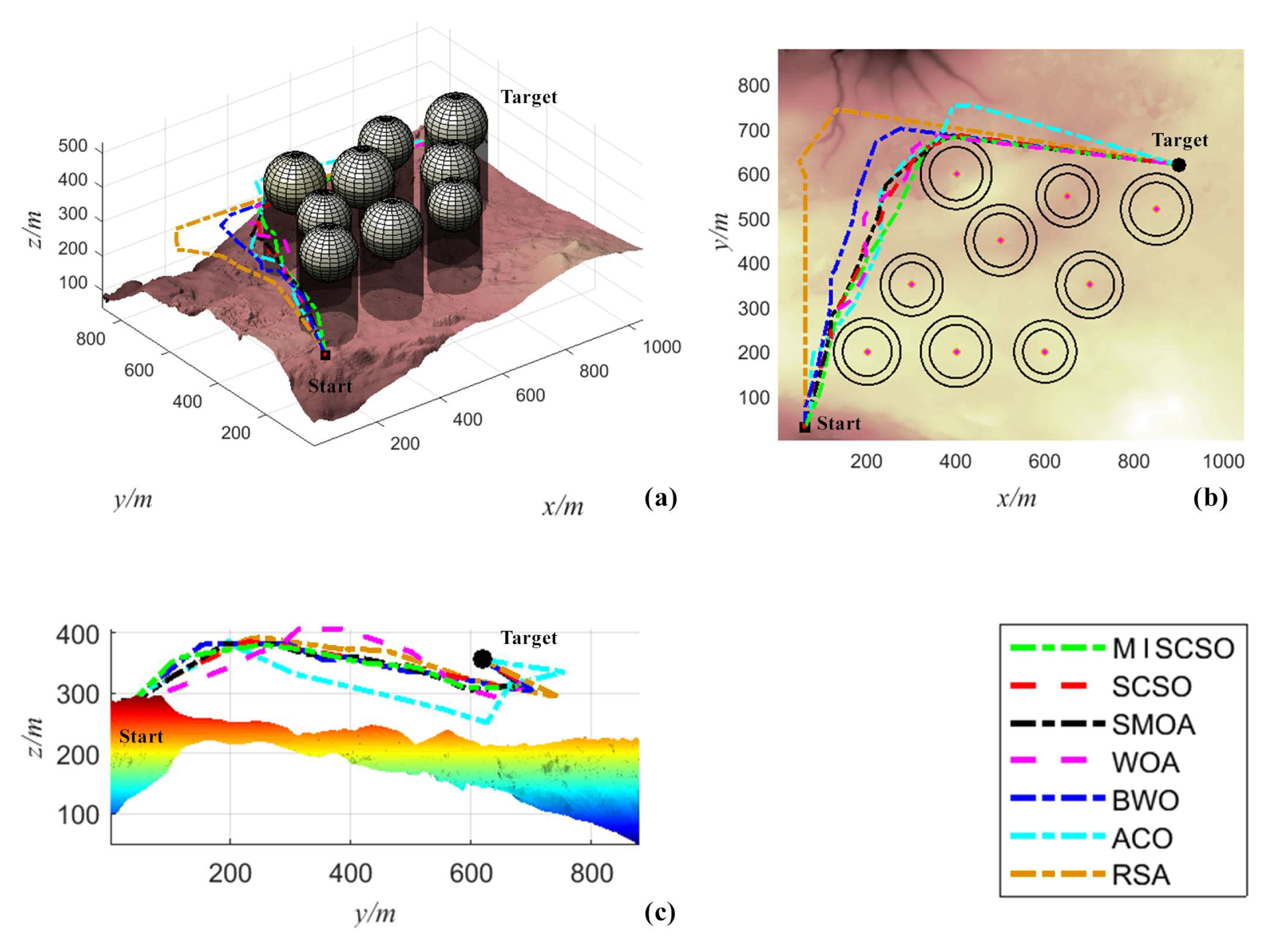
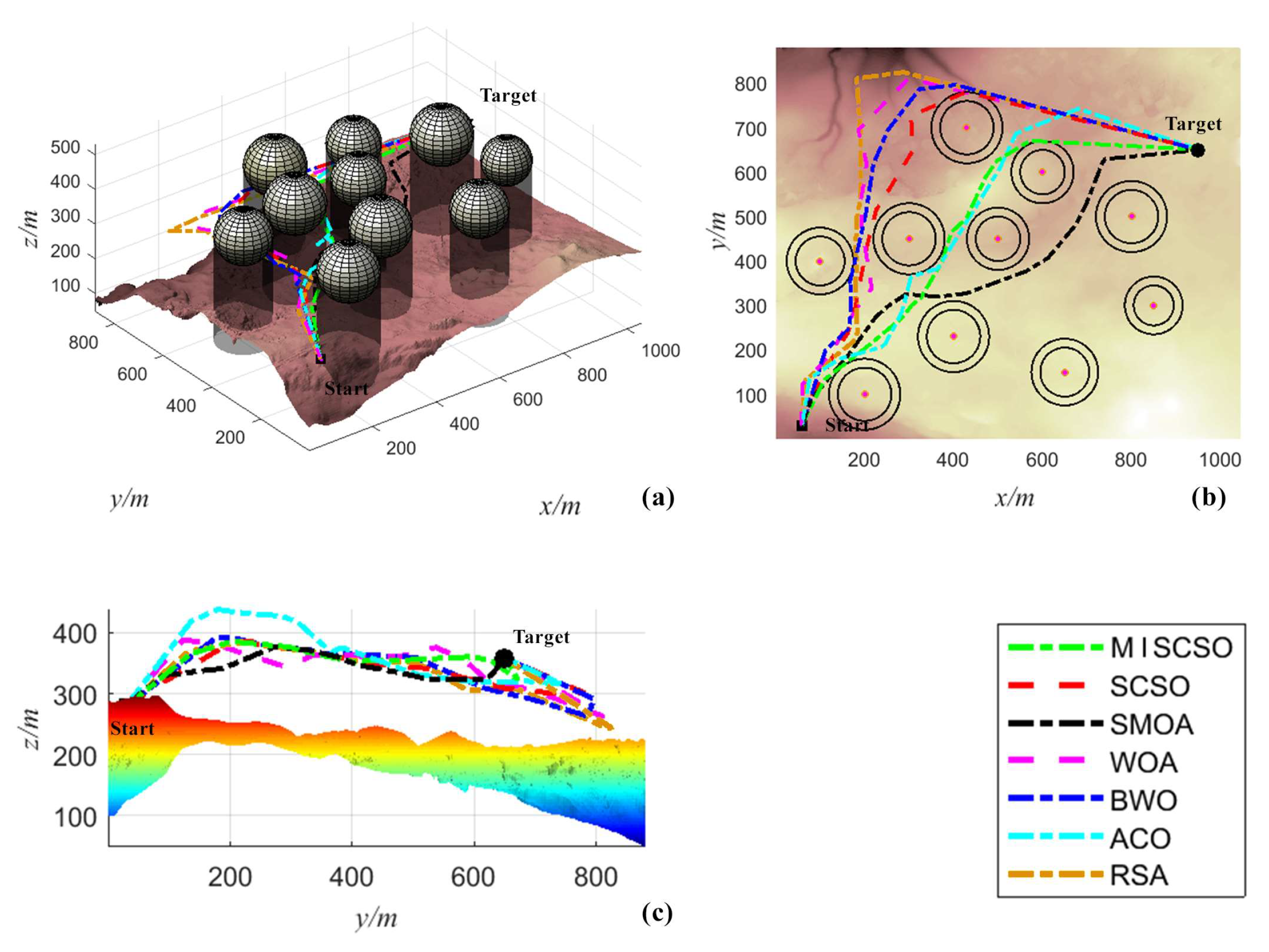
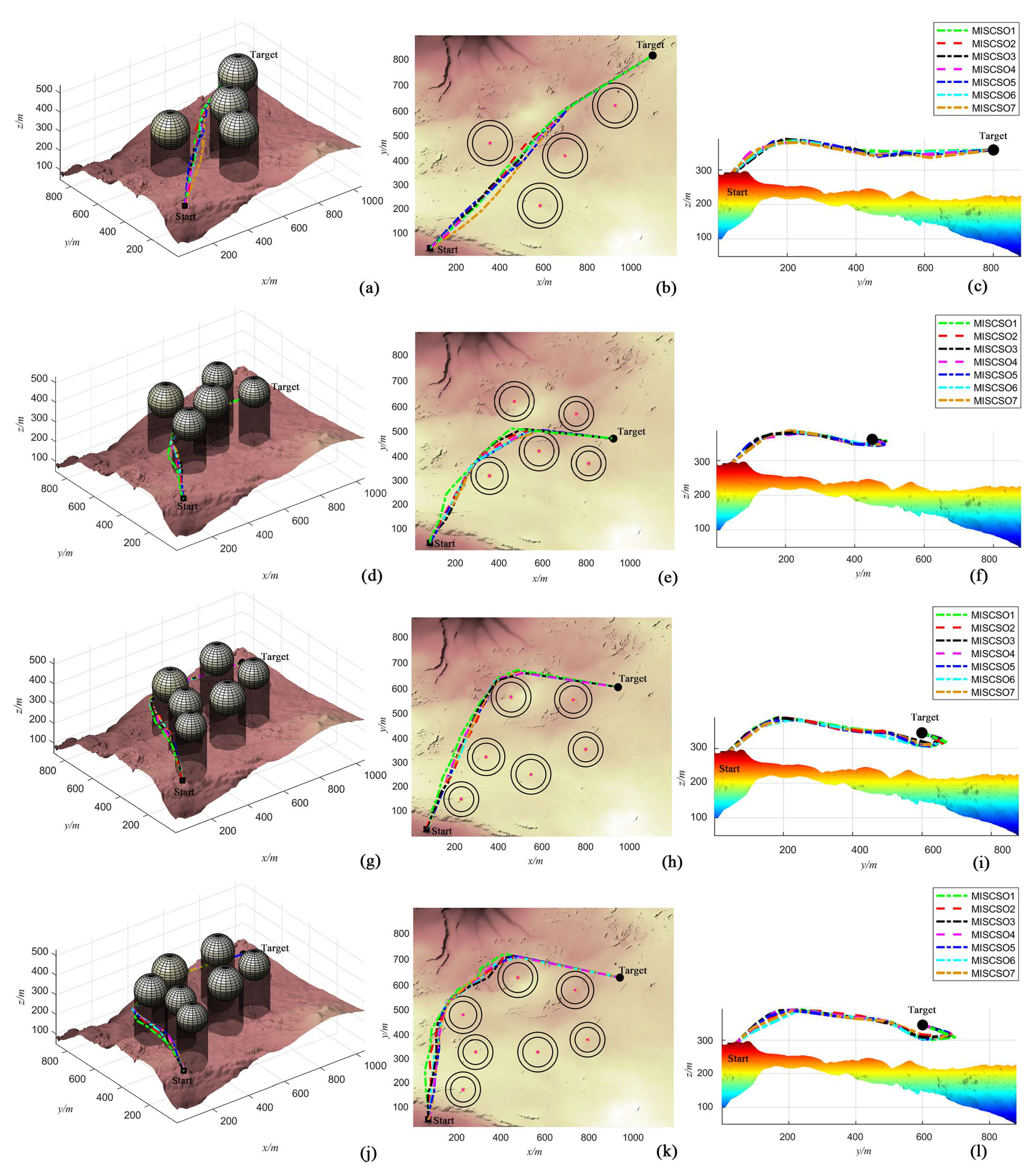
3.2. UAV Three-Dimensional Path Planning

To validate the effectiveness of the MISCSO algorithm in solving UAV path planning problems, seven different three-dimensional environment models were designed in this study, each with varying numbers of obstacles. In addition to the MISCSO algorithm, the SCSO, SMOA, WOA, BWO, ACO, and RSA algorithms were also selected for comparison. Figure 12, Figure 13, Figure 14, Figure 15, Figure 16, Figure 17 and Figure 18 show the constructed three-dimensional environments, where black square icons indicate the starting point of the trajectory, black circular icons indicate the destination point of the trajectory, brown areas represent baseline terrain models and mountain models, and gray-black cylindrical parts simulate obstacles. Figure 12, Figure 13, Figure 14, Figure 15, Figure 16, Figure 17 and Figure 18b,c show the top-down view and side view of the seven algorithms in the same scenario. It can be observed from the figures that all seven algorithms are able to find flight paths from the starting point to the destination.
In Figure 12b, it can be observed that the flight paths obtained by the RSA, BWO, SCSO, and WOA algorithms deviate significantly. The paths planned by the ACO, SMOA, and MISCSO algorithms are similar, but further examination of Figure 12a,c reveals that the flight height variation of the path planned by the MISCSO algorithm is relatively small and the path is relatively smooth. In Figure 13b, the seven algorithms show height overlap in the later part of the flight path, but in the first half, the paths planned by the RSA, BWO, and ACO algorithms are more tortuous and time-consuming, while the paths planned by the SMOA, SCSO, WOA, and MISCSO algorithms are relatively shorter. Among them, the flight path planned by the MISCSO algorithm maintains the shortest distance to obstacles during flight, demonstrating the sensitivity of the proposed algorithm in obstacle avoidance. In Figure 13c, the flight height planned by the MISCSO and SCSO algorithms is more stable. In Figure 14b,c, all seven algorithms choose to pass obstacles from the left side to reach the destination. The flight paths planned by the ACO, RSA, and WOA algorithms deviate in the first half of the path compared to other algorithms, while the remaining algorithms show similar path lengths and flight heights. From Figure 15b, it can be seen that when facing complex environments, the WOA algorithm and SMOA algorithm choose flight paths that differ from other algorithms. Figure 15c reveals that the WOA algorithm increases flight height and flies along a route closer to obstacles in order to plan a shorter path length, but this also increases the likelihood of encountering danger and collisions. It is clear from Figure 15b that the SMOA algorithm plans a longer path length, which is not the optimal choice. The RSA algorithm, with its large turning angles, is prone to collision accidents. Among the remaining four algorithms, whether in terms of path length or flight height, the MISCSO algorithm performs better than the others. In Figure 15b, the flight path planned by the WOA algorithm involves more turns, making it more convoluted and less smooth. Additionally, in Figure 16c, it can be observed that the WOA algorithm experiences significant fluctuation in flight height, indicating unstable path planning. The differences in flight height planning among the other algorithms are minimal, with the MISCSO algorithm having relatively shorter path lengths and smoother path planning. From Figure 17b, it can be seen that as obstacles increase and the distance between obstacles decreases, all algorithms choose to navigate around obstacles from the left, similar to Figure 14. The RSA algorithm still exhibits the issue of large turning angles, while the ACO and BWO algorithms deviate from the optimal path. In Figure 17c, the WOA and ACO algorithms show significant fluctuations in flight height, making them unsuitable for use as flight paths in practical scenarios. In Figure 18c, the RSA, WOA, BWO, and SCSO algorithms smoothly navigate from the outside of obstacles to the endpoint at a stable flight height. However, as seen in Figure 18b, these four algorithms plan longer paths, with the SCSO algorithm even colliding with obstacles. The ACO and MISCSO algorithms demonstrate higher path quality compared to the SMOA algorithm, but in Figure 18c, the ACO algorithm shows significant early-stage fluctuations in flight height. Therefore, the MISCSO algorithm provides a superior flight path planning solution.
In general, the improved MISCSO algorithm has found better paths in various complex environments, not only avoiding threat zones but also consistently maintaining a stable flight height to cross obstacles, significantly reducing the drone’s flight distance. Additionally, the paths planned by the MISCSO algorithm are smoother than those of other algorithms and can flexibly navigate around obstacles, thereby reducing the risk of collisions with mountains, threat zones, and other drones.
To evaluate the performance of the proposed algorithm on the model, metrics such as mean, best value, standard deviation, and worst value were used to analyze the algorithm’s adaptability and accuracy. Table 2 summarizes the mean, best value, standard deviation, and worst value for MISCSO and the six other algorithms.
When the number of obstacles is four, the SCSO, SMOA, and MISCSO algorithms show minimal differences in mean, best value, and worst value, while the WOA, BWO, and RSA algorithms slightly lag behind these three. The ACO algorithm exhibits the highest fluctuation, with the maximum standard deviation reaching ten to the power of three. Although the SCSO algorithm has the smallest standard deviation, the MISCSO algorithm outperforms the SCSO algorithm in the other three metrics. When the number of obstacles is five, the MISCSO algorithm excels in mean, best value, standard deviation, and worst value compared to the other six algorithms, indicating that the four improvement strategies effectively enhance the algorithm’s optimization accuracy and stability. Among the other six algorithms, the SCSO algorithm achieves the best results, followed by SMOA and WOA, highlighting the significant advantage of the cat swarm optimization algorithm in three-dimensional path planning. When the number of obstacles is six, although the results obtained by the SMOA and SCSO algorithms are competitive, the MISCSO algorithm offers optimal value, the highest stability, and the best numerical performance. When the number of obstacles is seven, the MISCSO algorithm excels in numerical performance, with a significantly better standard deviation than the other algorithms, followed by SCSO and SMOA, with the ACO algorithm showing the worst numerical performance. When the number of obstacles is eight, the MISCSO algorithm exhibits the best average and best values, providing accurate optimal results. The BWO algorithm has the smallest standard deviation, but the difference between MISCSO and BWO is minimal. Additionally, all other metrics of the MISCSO algorithm surpass those of the BWO algorithm. Although the ACO algorithm achieves the best worst value result, it has the worst standard deviation, even reaching ten to the power of three. When the number of obstacles is nine, the optimization capabilities of all algorithms decrease with an increase in obstacle quantity, but the MISCSO algorithm can still find precise solutions. When the number of obstacles is 10, the stability of the algorithms declines, with an increase in standard deviation values. While the MISCSO algorithm does not have the best standard deviation, it outperforms other algorithms in all other metrics. The SCSO algorithm follows, with the SMOA, BWO, and RSA algorithms showing minor differences. The WOA and ACO algorithms exhibit larger errors.
From Table 2, it is evident that regardless of the complexity of the environment, the MISCSO algorithm consistently achieves the optimal solution, demonstrating superior performance in discovery. Furthermore, the standard deviation of the MISCSO algorithm is generally better than that of the other six algorithms, indicating its robust stability. Compared numerically with the other six algorithms, the proposed MISCSO algorithm exhibits more prominent advantages and can adapt to more complex problems.
Figure 19 shows the iteration curves of the fitness functions of the seven algorithms under different models after 150 iterations. It is clear from Figure 19 that the MISCSO algorithm proposed in this paper has the smallest average fitness function value in the later stages of the iterations, demonstrating good performance and confirming its superior ability to adaptively search the feature space compared to other algorithms. In Figure 19d–g, as the number of obstacles increases, the environment becomes more complex, and the advantage of the MISCSO algorithm becomes more apparent. Not only can it complete fast iterations, but it also achieves greater accuracy in finding the optimal solution compared to other algorithms. In Figure 19, the ACO algorithm stagnates during iterations in (a) to (f), getting trapped in local optima, while the RSA algorithm iterates continuously in a step-like manner, only finding better solutions in the later stages of the iteration in (d) and (g), with slow convergence speed. Although the WOA algorithm converges quickly, it, like the ACO algorithm, is prone to getting trapped in local optima. The SMOA algorithm, BWO algorithm, and SCSO algorithm are similar, but in Figure 19b,f, the MISCSO algorithm significantly outperforms the SMOA and BWO algorithms in terms of both iteration speed and fitness function values.
In order to analyze the distribution characteristics of the improved algorithm in the seven models, box plots were drawn based on the independently solved results of each algorithm, as shown in Figure 20. It is evident from Figure 20 that the MISCSO algorithm has the smallest median, indicating the superior quality of solutions compared to the other algorithms. Additionally, as the difficulty of the models increases, the median of the other algorithms continues to rise, along with an increase in dispersion. However, the solutions obtained by the MISCSO algorithm remain concentrated and exhibit good stability. In Figure 20g, under the most complex model, the dispersion of the other algorithms is most pronounced, while the MISCSO algorithm still finds the optimal solution with minimal dispersion. It can be seen that the proposed MISCSO algorithm in this study demonstrates strong robustness, stability, and accuracy.
Sensitivity analysis, as a critical component of algorithm assessment, examines the robustness and resilience of algorithms under varying parameter and scenario configurations. In this study, an in-depth sensitivity analysis was conducted on the MISCSO algorithm, with a specific focus on the impact of population size (Pop) and the maximum number of iterations (M) on the optimization of 3D UAV trajectories. By scrutinizing the algorithm’s performance across different parameter settings, a comprehensive understanding of its applicability and dependability can be acquired, thereby offering valuable insights for further algorithm refinement.

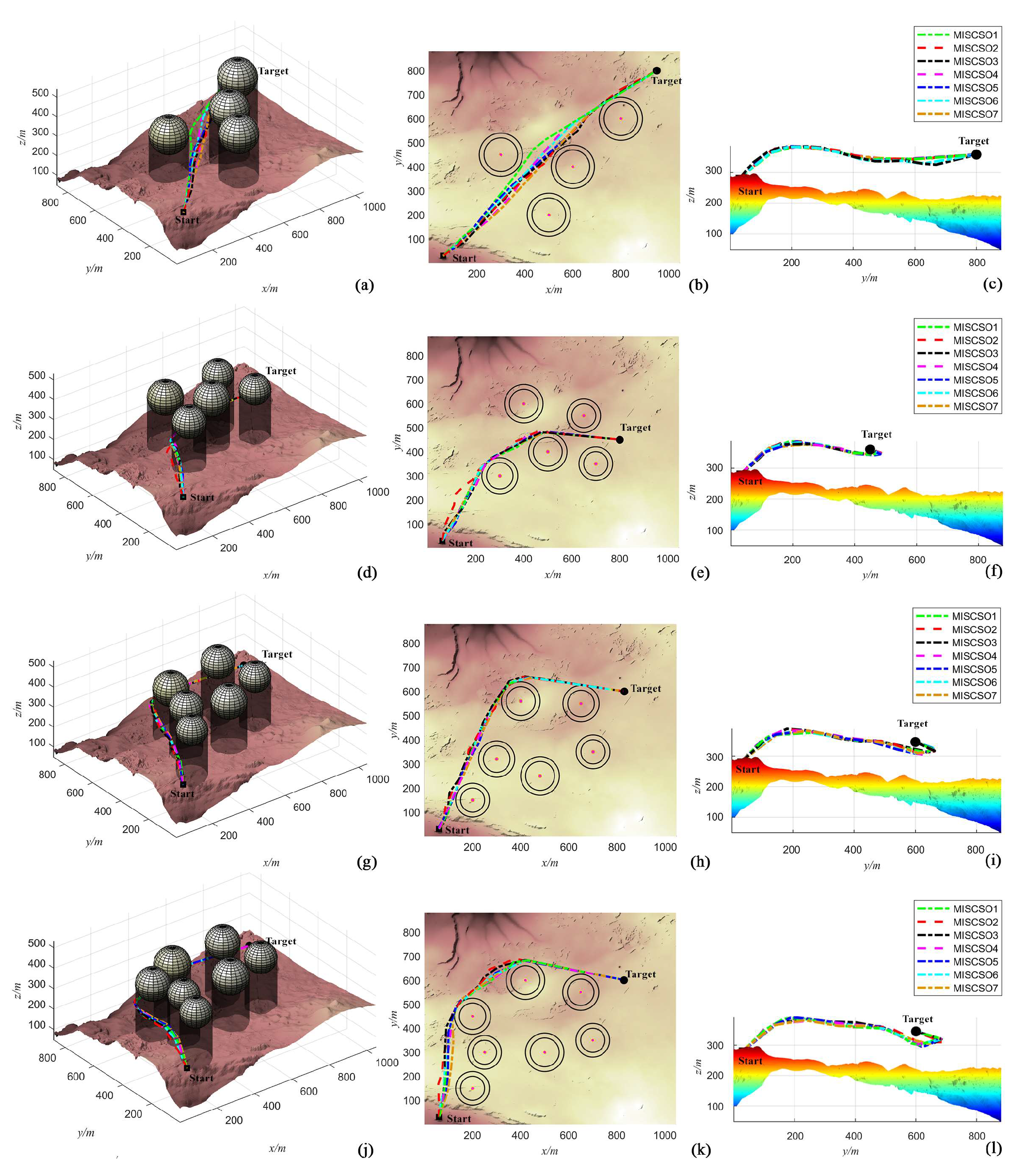
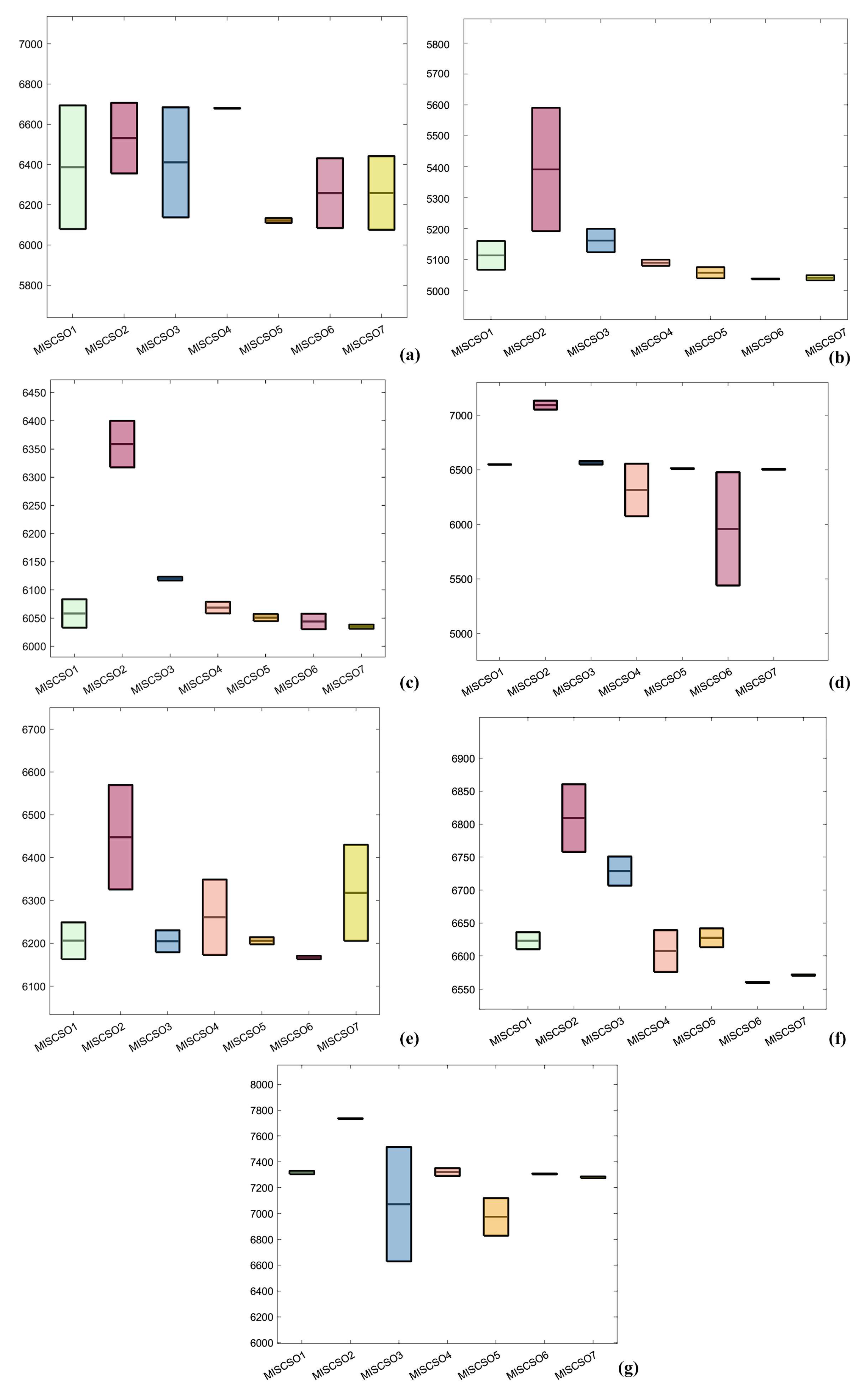
3.2.1. Population Size (Pop)

Keeping all other parameters constant, the MISCSO algorithm was tested with varying population sizes as follows: MISCSO1 (Pop = 300), MISCSO2 (Pop = 100), MISCSO3 (Pop = 200), MISCSO4 (Pop = 400), MISCSO5 (Pop = 500), MISCSO6 (Pop = 600), and MISCSO7 (Pop = 700). Table 3 presents the obstacle avoidance data of the proposed algorithm with varying population sizes under different numbers of obstacles. This analysis aims to investigate how the performance of the algorithm is affected by varying the size of the population.
From Table 3, it can be observed that with an increase in the population size, the average, best, and worst values do not differ significantly when the number of obstacles ranges from 4–7, while the standard deviation shows some fluctuation. Particularly, when the number of obstacles is four, although there is some deviation in the STD, the difference between the worst and best values is not significant. Furthermore, the running time of the algorithm increases with an increase in the population size. As shown in Figure 21, the MISCSO algorithm demonstrates similar running paths when facing the same obstacle with different population sizes. For obstacle numbers between 8–10, the differences in the best, average, and worst values remain relatively small, with the running time increasing as the population size increases.
An analysis of the performance of the MISCSO algorithm in environments with 4–10 obstacles reveals that an increase in the number of obstacles can impact the algorithm’s convergence speed, stability, and ability to find optimal solutions. It is observed that when the number of obstacles ranges from 4–7, the algorithm is able to find good solutions in a relatively short amount of time. Figure 22 indicates that algorithms with different population sizes exhibit similar trajectory fluctuations under the same number of obstacles. In Figure 23a, although different population sizes may lead to some deviation in the best solutions found, the fitness value deviation remains minimal. Figure 23e–g demonstrates that, as the number of obstacles increases, the exploration of optimal solutions becomes more challenging, leading to algorithm instability. The algorithm curve exhibits complex fluctuations in the early stage, and during the process of finding the optimal solution, there may be jumps or getting stuck in local optimal solutions. However, it eventually converges to satisfactory values. Figure 24 represents box plots of MISCSO algorithms under different numbers of obstacles for various Pop.

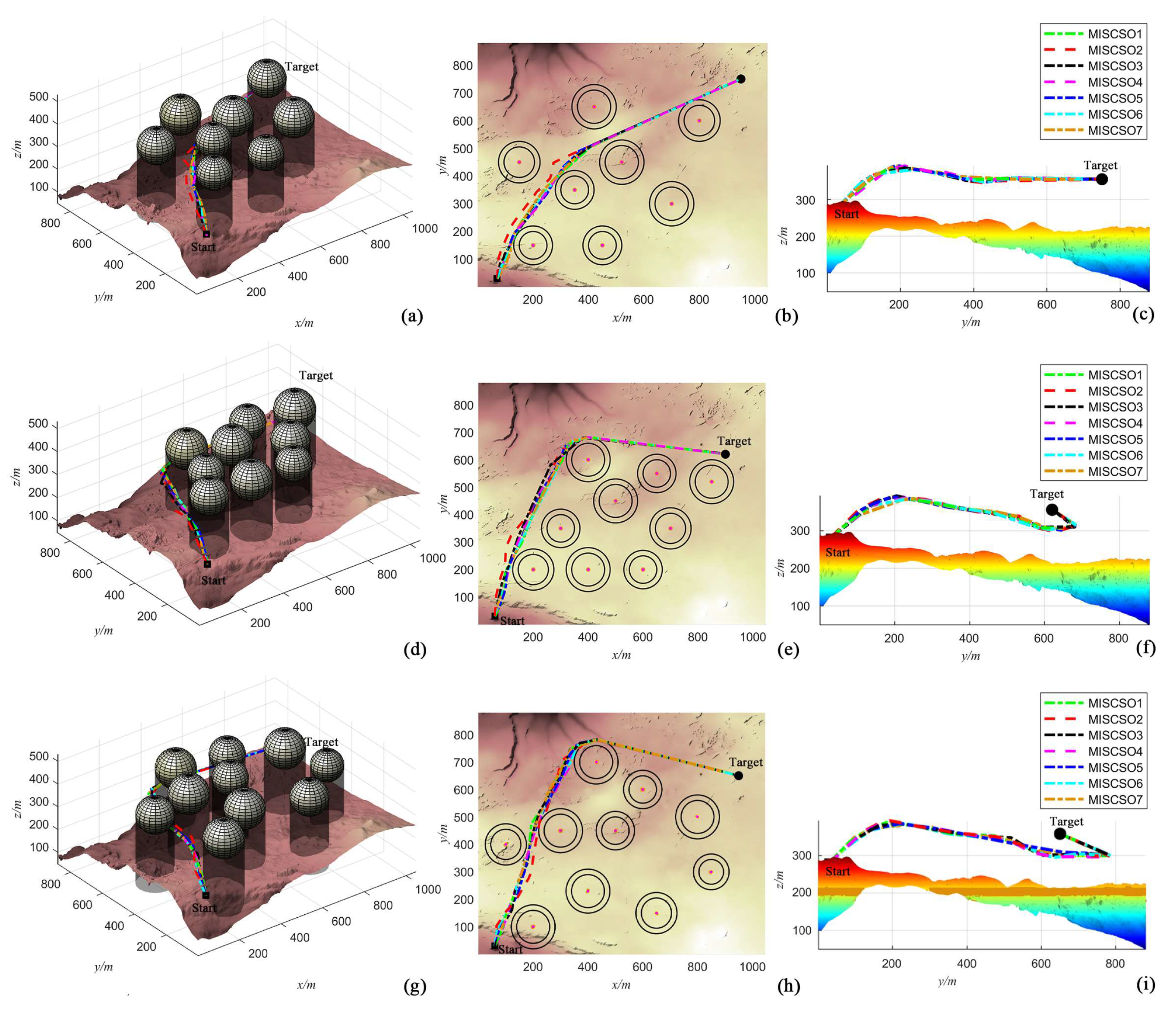
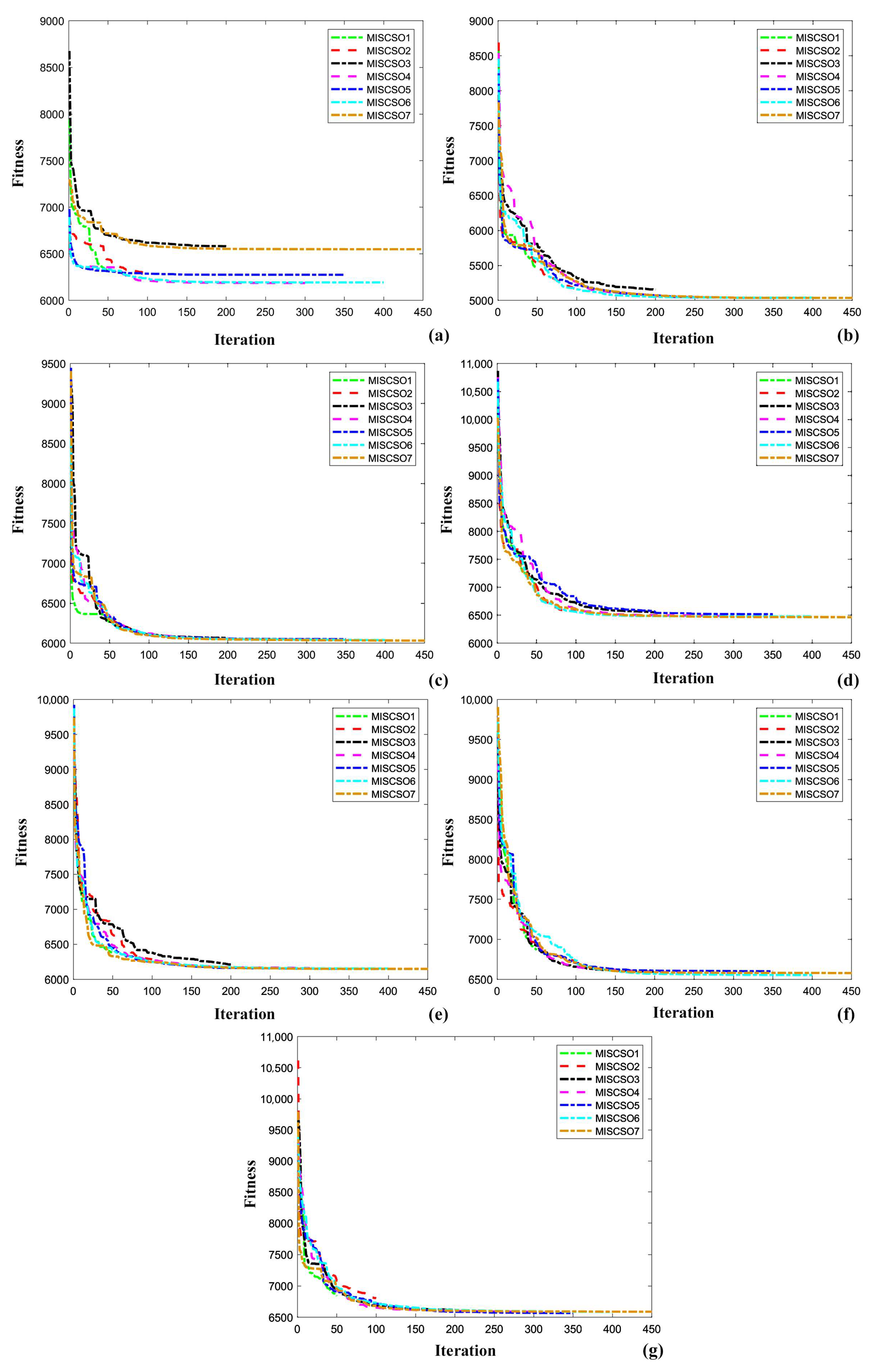
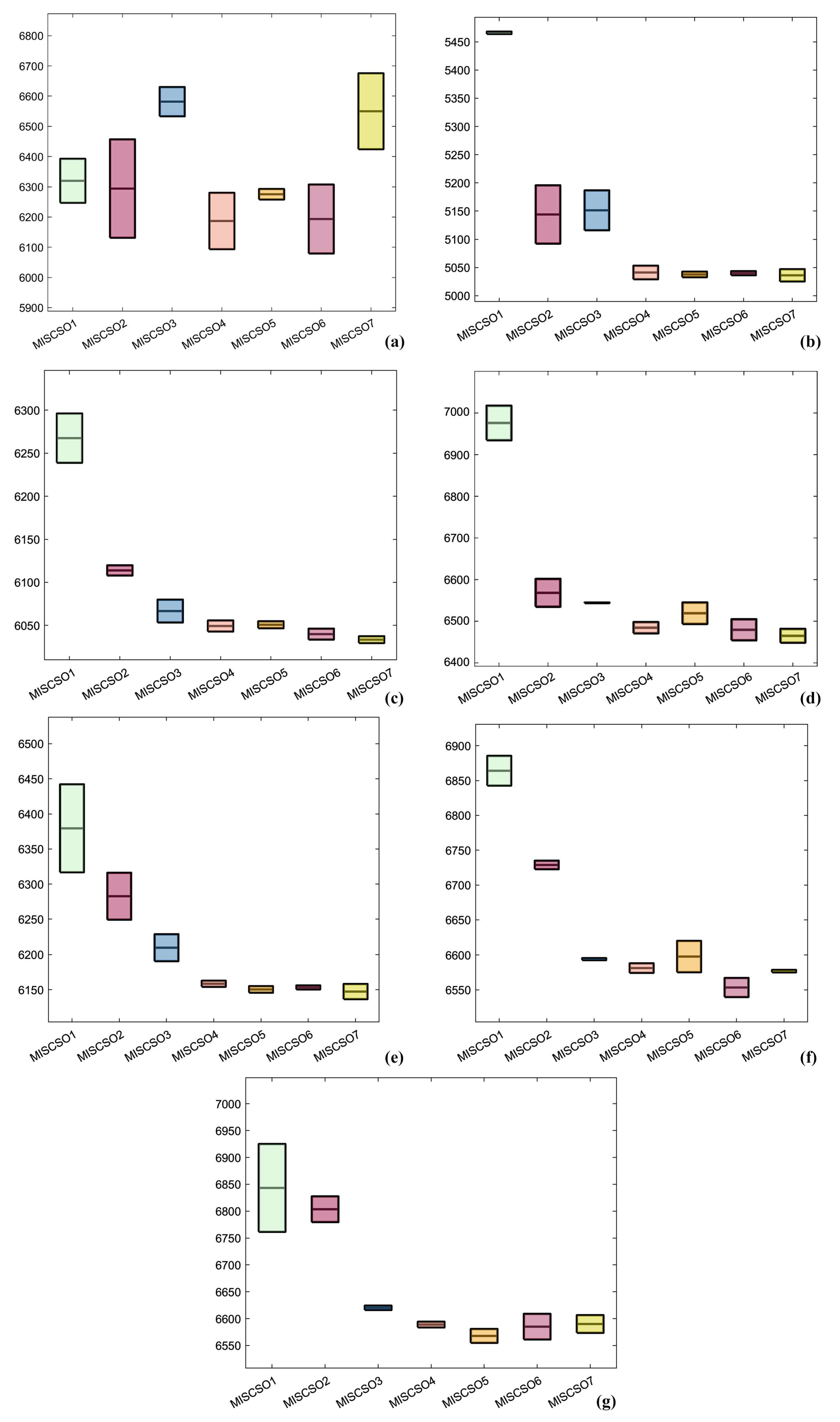
3.2.2. Maximum Number of Iterations (M)

Using varying maximum numbers of iterations (M), the MISCSO algorithm was tested with the following configurations: MISCSO1 (M1 = 50), MISCSO2 (M2 = 100), MISCSO3 (M3 = 200), MISCSO4 (M4 = 300), MISCSO5 (M5 = 350), MISCSO6 (M6 = 400), and MISCSO7 (M7 = 450). Table 3 showcases the obstacle avoidance data of the proposed algorithm when applied with different population sizes and varying numbers of obstacles while keeping all other parameters constant.
Combining Table 4 with Figure 25 and Figure 26, it can be observed that for the cases where the number of obstacles is either four or ten, the average, best, and worst values generated by the MISCSO algorithm show little deviation, with a small standard deviation indicating a consistent performance in finding the optimal path. However, as the number of iterations increases, the algorithm’s runtime also increases. Figure 27 illustrates how the adaptability of the MISCSO algorithm changes under varying numbers of obstacles and different conditions of M with respect to the number of iterations, while Figure 28 presents a box plot detailing the algorithm’s performance under different obstacle scenarios. Consequently, when either the population size or the maximum number of iterations is increased individually, the performance metrics of the MISCSO algorithm—including best, worst, average values, and standard deviation—show insignificant differences, suggesting a certain level of stability and adaptability. Nevertheless, the algorithm’s runtime demonstrates an upward trend, indicating that in more complex environments, it requires additional time to explore the solution space and identify the optimal path. Despite this, the algorithm can still achieve relatively good solutions through high-quality path planning.

4. Conclusions

This article first introduces the cost model of UAV flight, then explains the principle of the SCSO algorithm and establishes a mathematical model. Addressing issues such as premature convergence, lack of population diversity, and poor convergence accuracy in the traditional Sand Cat Optimization (SCSO) algorithm, improvement methods are proposed, and detailed explanations of the algorithm’s enhancement strategies are provided. CEC2017 benchmark functions are selected for comparison with six popular algorithms. It was found that the improved MISCSO algorithm outperformed other algorithms in terms of fitness value. Additionally, the algorithm’s convergence speed and accuracy were significantly improved compared to the original algorithm. By simulating flight path planning in a three-dimensional environment, it was discovered that the MISCSO algorithm not only can generate relatively optimal paths but can also significantly enhance the smoothness of flight altitude and the speed of optimization. The effects become more pronounced with the increasing complexity of the environment. Applying the improved algorithm to flight path-planning experiments demonstrated that the MISCSO algorithm has a relatively faster convergence speed, is less likely to get trapped in obstacle scenarios, shows high adaptability in complex environments, and meets practical requirements by planning a safe and reliable high-quality flight path.

Author Contributions

L.L. (Lili Liu): investigation, methodology, software and writing—original draft. Y.L.: investigation, resources, visualization, and validation. B.Y.: resources, visualization, and validation. L.Y.: resources, software and visualization. J.Z.: funding acquisition, methodology and supervision. Y.C.: investigation, visualization and validation. L.L. (Longhai Li): conceptualization, methodology, funding acquisition and writing—review and editing. All authors have read and agreed to the published version of the manuscript.

Funding

This work was supported by the National Natural Science Foundation of China (grant No. 51975516); the Natural Science Foundation of the Jiangsu Higher Education Institutions of China (grant No. 21KJB460033); Science Research Project of Xuzhou University of Technology (grant No. KC21002).

Institutional Review Board Statement

Not applicable.

Informed Consent Statement

Not applicable.

Data Availability Statement

The original contributions presented in the study are included in the article, further inquiries can be directed to the corresponding author.

Conflicts of Interest

The authors declare no conflicts of interest.

Appendix A

Table A1. Unimodal Functions.
Function NameMetricMISCSOSCSOSMOAWOABWOACORSA
f1Best100.041089.446.17 × 1077.91 × 1043.79 × 107194.188.95 × 109
STD0.042.41 × 1054.42 × 1073.23 × 1058.75 × 1063657.951.47 × 109
Average100.091.19 × 1051.08 × 1083.94 × 1054.82 × 1071922.781.03 × 1010
Worst100.145.49 × 1051.66 × 1089.17 × 1056.09 × 1078465.101.27 × 1010
f2Best300.00368.281684.30563.21525.00990.975485.49
STD0.002086.981632.341428.02213.28726.611983.29
Average300.001994.094097.541565.74886.181762.157454.23
Worst300.005506.346119.303912.051061.432914.761.06 × 104
Table A2. Simple Multimodal Functions.
Function NameMetricMISCSOSCSOSMOAWOABWOACORSA
f3Best400.00400.58410.87401.61408.19403.27577.91
STD0.0026.754.6328.971.370.09503.57
Average400.00427.00414.95419.81410.13403.41969.93
Worst400.00471.48422.80469.99412.06403.501730.58
f4Best504.98517.96522.24540.83517.35529.41553.71
STD2.097.947.0920.963.102.8021.84
Average508.62529.36534.56562.13521.76531.38579.47
Worst510.02536.85540.41595.15525.70536.31607.32
f5Best600.01606.38605.23626.22602.97600.00637.38
STD0.0314.802.6917.180.630.004.21
Average600.04620.12608.02637.27603.66600.00641.39
Worst600.08644.72611.77666.98604.61600.00648.10
f6Best715.70742.96756.26750.62730.31738.81782.02
STD5.7210.061.9813.324.362.3012.74
Average723.20753.23758.78768.13733.68741.65797.29
Worst730.36765.40760.72783.36741.05743.40815.64
f7Best807.96823.94829.32819.92810.83811.38835.11
STD5.997.074.8017.983.408.2010.43
Average813.73833.82836.18842.10815.51825.94845.17
Worst821.89842.38840.56870.12820.06830.94860.99
f8Best900.00915.42982.621017.30907.41900.001356.63
STD4.4738.0327.47608.374.120.00107.33
Average903.45959.621013.121539.96911.70900.001451.14
Worst909.231015.331042.632424.16917.17900.001627.26
f9Best1498.561499.792092.301808.041215.732648.942073.84
STD169.73230.02122.48186.28171.73123.31577.17
Average1650.381878.552303.801990.471361.792758.422599.13
Worst1942.862127.952406.512283.281636.002894.873333.27
Table A3. Hybrid Functions.
Function NameMetricMISCSOSCSOSMOAWOABWOACORSA
f10Best1104.501112.491135.961129.371114.431106.152352.44
STD11.5676.6122.1328.348.761.111386.97
Average1116.261176.791160.551160.831120.021107.693510.24
Worst1131.581309.881195.631186.241135.551108.815682.04
f11Best1331.161.93 × 1052.32 × 1065.41 × 1042.25 × 1051.31 × 1047.86 × 107
STD138.739.80 × 1052.98 × 1061.77 × 1062.38 × 1052.96 × 1041.63 × 108
Average1459.821.44 × 1064.75 × 1061.66 × 1065.58 × 1052.90 × 1041.64 × 108
Worst1660.872.52 × 1068.82 × 1063.91 × 1068.55 × 1058.17 × 1044.55 × 108
f12Best1306.422927.926992.053592.027090.006109.623.80 × 106
STD2.747414.255506.732.78 × 1043240.476777.054.74 × 107
Average1310.548469.541.42 × 1043.07 × 1041.07 × 1041.18 × 1045.22 × 107
Worst1314.031.90 × 1042.24 × 1046.66 × 1041.39 × 1042.11 × 1041.05 × 108
f13Best1402.791459.581487.101537.081430.811506.611581.91
STD6.491667.3538.40243.10109.49868.782101.40
Average1407.722220.641527.481683.291539.852345.874872.09
Worst1418.615203.231583.492105.321707.763633.266825.12
f14Best1501.181582.071916.712860.871525.792988.624817.00
STD3.81399.28182.052039.761014.795912.527440.52
Average1504.251926.982145.066213.462237.438474.089200.37
Worst1510.882415.232345.938302.913983.131.85 × 1042.24 × 104
f15Best1600.551744.281639.911742.891606.561618.221862.44
STD104.64132.1730.96176.0052.0941.98145.84
Average1674.201851.251677.871885.091633.921671.752044.53
Worst1838.232004.661716.072142.061726.731720.792190.36
f16Best1701.431748.291753.261770.061728.691733.311795.26
STD9.6910.255.8934.0310.2414.6652.28
Average1717.931763.881761.591800.621739.321749.001832.23
Worst1725.861775.751768.651856.041756.111770.331920.24
f17Best1802.014334.471.33 × 1048439.074295.596.26 × 1043.30 × 105
STD11.541.30 × 1042.21 × 1049851.291.31 × 1046.71 × 1044.73 × 106
Average1810.241.43 × 1043.48 × 1042.42 × 1041.68 × 1041.66 × 1054.22 × 106
Worst1830.463.32 × 1046.79 × 1043.52 × 1043.82 × 1042.38 × 1059.99 × 106
f18Best1901.091911.971974.902905.192205.694078.992.16 × 104
STD0.9539.81111.711.26 × 105427.534027.014.93 × 105
Average1901.651950.772062.287.53 × 1042708.827314.754.37 × 105
Worst1903.332016.302220.712.96 × 1053270.7714,328.771.06 × 106
f19Best2002.482058.372062.102081.712028.742020.022215.51
STD9.3052.957.8883.983.410.2831.00
Average2009.282110.802070.892155.212032.062020.242256.23
Worst2025.312170.452080.422279.132036.312020.682289.92
Table A4. Composition Functions.
Function NameMetricMISCSOSCSOSMOAWOABWOACORSA
f20Best2200.002208.932207.012227.122202.602280.192250.45
STD64.2856.666.8062.831.8722.0858.39
Average2269.982308.912214.332336.852204.512319.072294.83
Worst2327.412343.762225.032382.402207.172335.052388.16
f21Best2300.902232.982312.532309.782233.282302.432785.73
STD1.2235.795.275.5936.48395.27253.15
Average2301.572295.332317.832315.482298.432480.322973.24
Worst2303.732321.332325.692324.322318.223187.393396.56
f22Best2608.252620.922635.972619.012618.612632.292669.38
STD4.949.052.3215.262.903.6119.53
Average2612.932635.292639.832632.672621.932636.752690.68
Worst2620.282645.812641.832657.002626.432640.642715.42
f23Best2734.302518.732585.002514.242527.262759.582824.45
STD4.18108.9497.30123.1397.482.8728.09
Average2740.152713.052673.602731.992577.972764.482852.38
Worst2745.892771.502779.262812.922752.092767.112897.88
f24Best2897.942913.462918.422907.332903.832943.983288.10
STD30.7235.717.1822.055.161.0656.89
Average2930.262942.922925.692927.192908.712945.163375.42
Worst2967.683000.742937.292951.262915.852945.973437.43
f25Best2900.002900.052972.533015.222921.193233.693430.28
STD50.2855.1917.58501.4817.1460.32455.92
Average2954.682959.362994.833907.672935.903308.364057.46
Worst3000.013013.103014.264183.292964.363378.754500.62
f26Best3073.473093.043077.953093.283090.353173.623119.34
STD1.9835.180.6949.711.5511.0475.81
Average3075.293112.743078.963123.753092.593190.493176.15
Worst3078.343174.963079.883211.813093.973200.003309.34
f27Best3194.533100.053223.883230.023116.713297.093812.87
STD55.59135.0721.8994.0528.681.0128.54
Average3259.463340.753263.033334.343153.363298.193852.27
Worst3300.003412.703273.013411.913180.493299.723885.93
f28Best3132.883157.133186.353179.143161.933227.183232.37
STD25.7044.7128.46155.9413.3129.15106.91
Average3150.073207.193208.043371.213172.003257.183351.24
Worst3195.473255.053256.363591.073194.553301.103473.92
f29Best3247.284828.623564.0714,381.738971.215391.902.02 × 106
STD1951.575.95 × 105201.261.25 × 1064.23 × 1044665.668.09 × 106
Average4155.553.04 × 1053708.901.48 × 1065.01 × 1049042.969.09 × 106
Worst7646.191.37 × 1064050.502.55 × 1061.00 × 1051.68 × 1041.89 × 107

References

  1. Huang, T.; Huang, D.; Qin, N.; Li, Y. Path planning and control of a quadrotor UAV based on an improved APF using parallel search. Int. J. Aerosp. Eng. 2021, 2021, 5524841. [Google Scholar] [CrossRef]
  2. Fu, G.; Gao, Y.; Liu, L.; Yang, M.; Zhu, X. UAV Mission Path Planning Based on Reinforcement Learning in Dynamic Environment. J. Funct. Space. 2023, 2023, 9708143. [Google Scholar] [CrossRef]
  3. Yuan, M.; Zhou, T.; Chen, M. Improved lazy theta* algorithm based on octree map for path planning of UAV. Def. Technol. 2023, 23, 8–18. [Google Scholar] [CrossRef]
  4. Guo, Y.; Liu, X.; Yang, Y.; Zhang, W. FC-RRT*: An Improved Path Planning Algorithm for UAV in 3D Complex Environment. ISPRS Int. J. Geo-Inf. 2022, 11, 112. [Google Scholar] [CrossRef]
  5. Li, W.; Wang, L.; Zou, W.; Cai, J.; He, H.; Tan, T. Path Planning for UAV Based on Improved PRM. Energies 2022, 15, 7267. [Google Scholar] [CrossRef]
  6. Li, J.; Liao, C.; Zhang, W.; Fu, H.; Fu, S. UAV Path Planning Model Based on R5DOS Model Improved A-Star Algorithm. Appl. Sci. 2022, 12, 11338. [Google Scholar] [CrossRef]
  7. Wang, X.; Cheng, M.; Zhang, S.; Gong, H. Multi-UAV Cooperative Obstacle Avoidance of 3D Vector Field Histogram Plus and Dynamic Window Approach. Drones 2023, 7, 504. [Google Scholar] [CrossRef]
  8. Ait-Saadi, A.; Meraihi, Y.; Soukane, A.; Ramdane-Cherif, A.; Gabis, A.B. A Novel hybrid Chaotic Aquila Optimization algorithm with Simulated Annealing for Unmanned Aerial Vehicles path planning. Comput. Electr. Eng. 2022, 69, 2093–2123. [Google Scholar] [CrossRef]
  9. Deng, L.; Chen, H.; Zhang, X.; Liu, H. Three-Dimensional Path Planning of UAV Based on Improved Particle Swarm Optimization. Mathematics 2023, 11, 1987. [Google Scholar] [CrossRef]
  10. Chen, Q.; He, Q.; Zhang, D. UAV Path Planning Based on an Improved Chimp Optimization Algorithm. Axioms 2023, 12, 702. [Google Scholar] [CrossRef]
  11. Zhang, R.; Li, S.; Ding, Y.; Qin, X.; Xia, Q. UAV Path Planning Algorithm Based on Improved Harris Hawks Optimization. Sensors 2022, 22, 5232. [Google Scholar] [CrossRef] [PubMed]
  12. Rajeev, K.; Laxman, S.; Rajdev, T. Novel Reinforcement Learning Guided Enhanced Variable Weight Grey Wolf Optimization (RLV-GWO) Algorithm for Multi-UAV Path Planning. Wirel. Pers. Commun. 2023, 131, 2093–2123. [Google Scholar]
  13. Saxena, P.; Tayal, S.; Gupta, R.; Maheshwari, A.; Kaushal, G.; Tiwari, R. Three-dimensional route planning for multiple unmanned aerial vehicles using Salp Swarm Algorithm. J. Exp. Theor. Artif. Intell. 2022, 35, 1059–1078. [Google Scholar]
  14. Wang, W.; Chen, Y.; Tian, J. SGGTSO: A Spherical Vector-Based Optimization Algorithm for 3D UAV Path Planning. Drones 2023, 7, 452. [Google Scholar] [CrossRef]
  15. Chen, H.; Liang, Y.; Meng, X. A UAV Path Planning Method for Building Surface Information Acquisition Utilizing Opposition-Based Learning Artificial Bee Colony Algorithm. Remote Sens. 2023, 15, 4312. [Google Scholar] [CrossRef]
  16. Meng, X.; Zhu, X.; Zhao, J. Obstacle Avoidance Path Planning Using the Elite Ant Colony Algorithm for Parameter Optimization of Unmanned Aerial Vehicles. Arab. J. Sci. Eng. 2023, 48, 2261–2275. [Google Scholar] [CrossRef]
  17. Shen, Q.; Zhang, D.; Xie, M.; He, Q. Multi-Strategy Enhanced Dung Beetle Optimizer and Its Application in Three-Dimensional UAV Path Planning. Symmetry 2023, 15, 1432. [Google Scholar] [CrossRef]
  18. Wu, X.; Xu, L.; Zhen, R.; Wu, X. Global and Local Moth-flame Optimization Algorithm for UAV Formation Path Planning Under Multi-constraints. Int. J. Control Autom. 2023, 21, 1032–1047. [Google Scholar] [CrossRef]
  19. Hayal, M.; Elsayed, E.; Kakati, D.; Singh, M.; Elfikky, A.; Boghdady, A.; Grover, A.; Mehta, S.; Mohsan, S.; Nurhidayat, I. Modeling and investigation on the performance enhancement of hovering UAV-based FSO relay optical wireless communication systems under pointing errors and atmospheric turbulence effects. Opt. Quantum Electron. 2023, 55, 1–23. [Google Scholar]
  20. Elsayed, E. Investigations on OFDM UAV-based free-space optical transmission system with scintillation mitigation for optical wireless communication-to-ground links in atmospheric turbulence. Opt. Quantum Electron. 2024, 56, 837. [Google Scholar] [CrossRef]
  21. Kvitko, D.; Rybin, V.; Bayazitov, O.; Karimov, A.; Karimov, T.; Butusov, D. Chaotic Path-Planning Algorithm Based on Courbage–Nekorkin Artificial Neuron Model. Mathematics 2024, 12, 892. [Google Scholar] [CrossRef]
  22. Li, C.; Huang, X.; Ding, J.; Song, K.; Lu, S. Global path planning based on a bidirectional alternating search A* algorithm for mobile robots. Comput. Ind. Eng. 2022, 168, 108123. [Google Scholar] [CrossRef]
  23. Wang, J.; Chi, W.; Li, C.; Wang, C.; Meng, M.Q.-H. Neural RRT*: Learning-Based Optimal Path Planning. IEEE T Autom. Sci. Eng. 2020, 17, 1748–1758. [Google Scholar] [CrossRef]
  24. Lopes, G.; Hoffman, D. An Optimized Breadth-First Search Algorithm for Routing in Optical Access Networks. IEEE Lat. Am. Trans. 2019, 17, 1088–1095. [Google Scholar] [CrossRef]
  25. Seyyedabbasi, A.; Kiani, F. Sand Cat swarm optimization: A nature-inspired algorithm to solve global optimization problems. Eng. Comput. 2022, 39, 2627–2651. [Google Scholar] [CrossRef]
  26. Farzad, K.; Sajjad, N.; Fateme, A.; Mine, A. Chaotic Sand Cat Swarm Optimization. Mathematics 2023, 11, 2340. [Google Scholar] [CrossRef]
  27. Wang, X.; Liu, Q.; Zhang, L. An Adaptive Sand Cat Swarm Algorithm Based on Cauchy Mutation and Optimal Neighborhood Disturbance Strategy. Biomimetics 2023, 8, 191. [Google Scholar] [CrossRef] [PubMed]
  28. Wu, D.; Rao, H.; Wen, C.; Jia, H.; Liu, Q.; Abualigah, L. Modified Sand Cat Swarm Optimization Algorithm for Solving Constrained Engineering Optimization Problems. Mathematics 2022, 10, 4350. [Google Scholar] [CrossRef]
  29. Yao, L.; Yang, J.; Yuan, P.; Li, G.; Lu, Y. Multi-Strategy Improved Sand Cat Swarm Optimization: Global Optimization and Feature Selection. Biomimetics 2023, 8, 492. [Google Scholar] [CrossRef] [PubMed]
  30. Qadir, Z.; Zafar, M.H.; Moosavi, S. Autonomous UAV-path planning optimization using metaheuristic approach for pre-disaster assessment. IEEE Internet Things 2021, 9, 12505–12514. [Google Scholar] [CrossRef]
  31. Seo, D.; Kang, J. Collision-avoided Tracking Control of UAV Using Velocity-adaptive 3D Local Path Planning. Int. J. Control Autom. Syst. 2023, 21, 231–243. [Google Scholar] [CrossRef]
  32. Jayaweera, H.; Hanoun, S. Path planning of unmanned aerial vehicles (UAVs) in windy environments. Drones 2022, 6, 101. [Google Scholar] [CrossRef]
  33. Ali, A.; Zhang, G.; Zhen, G. Path planning of multiple UAVs using MMACO and DE algorithm in dynamic environment. Meas. Control 2023, 56, 459–469. [Google Scholar] [CrossRef]
  34. Kyriakakis, N.A.; Marinaki, M.; Matsatsinis, N. A cumulative unmanned aerial vehicle routing problem approach for humanitarian coverage path planning. Eur. J. Oper. Res. 2022, 300, 992–1004. [Google Scholar] [CrossRef]
  35. Balasubramanian, E.; Elangovan, E.; Tamilarasan, P.; Kanagachidambaresan, G.R.; Chutia, D. Optimal energy efficient path planning of UAV using hybrid MACO-MEA* algorithm: Theoretical and experimental approach. J. Ambient. Intell. Humaniz. Comput. 2023, 14, 13847–13867. [Google Scholar] [CrossRef] [PubMed]
  36. Khan, M.T.R.; Saad, M.M.; Ru, Y.; Seo, J.; Kim, D. Aspects of UAV path planning: Overview and applications. Int. J. Commun. Syst. 2021, 34, e4827. [Google Scholar] [CrossRef]
  37. Deng, M.; Yang, Q.; Peng, Y. A Real-Time Path Planning Method for Urban Low-Altitude Logistics UAVs. Sensors 2023, 23, 747–753. [Google Scholar] [CrossRef] [PubMed]
  38. Chen, J.; Zhang, R.; Zhao, H. Path planning of multiple unmanned aerial vehicles covering multiple regions based on minimum consumption ratio. Aerospace 2023, 10, 93–102. [Google Scholar] [CrossRef]
  39. Chen, Q.; Li, Q.; Li, R. UAV Network Path Planning and Optimization Using a Vehicle Routing Model. Remote Sens. 2023, 15, 2227–2247. [Google Scholar] [CrossRef]
  40. Luo, J.; Tian, Y.; Wang, Z. Research on Unmanned Aerial Vehicle Path Planning. Drones 2024, 8, 51–64. [Google Scholar] [CrossRef]
  41. Phung, M.D.; Ha, Q. Safety-enhanced UAV path planning with spherical vector-based particle swarm optimization. Appl. Soft Comput. 2021, 107, 107376. [Google Scholar] [CrossRef]
Figure 1. Initial stage of the SCSO algorithm.
Wevj 15 00244 g001
Figure 2. Random angle variations.
Wevj 15 00244 g002
Figure 3. Position Update Diagram.
Wevj 15 00244 g003
Figure 4. UAV flight path diagram.
Wevj 15 00244 g004
Figure 5. Calculation of yaw angle and pitch angle.
Wevj 15 00244 g005
Figure 6. Average fitness curves of different algorithms. Parts (a,b) represent f1 and f2, which correspond to unimodal Functions, while parts (ch) represent f3 to f8, which correspond to multimodal Functions.
Wevj 15 00244 g006
Figure 7. Average fitness curves of different algorithms. Part (a) represents f9, which corresponds to Shifted and Rotated Schwefel’s Functions, while parts (bj) represent f10 to f18, which correspond to hybrid Functions.
Wevj 15 00244 g007
Figure 8. Average fitness curves of different algorithms. Part (a) represents f19, which corresponds to Hybrid Function 10 (N = 6), while parts (bk) represent f20 to f29, which correspond to composition functions.
Wevj 15 00244 g008
Figure 9. Box plots of various algorithms. Sections (a,b) depict f1 and f2, respectively, corresponding to unimodal functions, while sections (ch) depict f3 to f8, corresponding to multimodal functions.
Wevj 15 00244 g009
Figure 10. Box plots of various algorithms. Section (a) depicts f9, corresponding to Shifted and Rotated Schwefel’s Functions, while sections (bj) depict f10 to f18, corresponding to hybrid functions.
Wevj 15 00244 g010
Figure 11. Box plots of various algorithms. Section (a) depicts f19, corresponding to hybrid function 10 (N = 6), while sections (bk) depict f20 to f29, corresponding to composition functions.
Wevj 15 00244 g011
Figure 12. Three-dimensional models of different algorithms with 4 obstacles. (a) 3D model; (b) top view, black circles represent the target locations, while the pink dots represent the centers of obstacles; (c) side view, different colors in (c) represent the different heights.
Wevj 15 00244 g012
Figure 13. Three-dimensional models of different algorithms with 5 obstacles. (a) 3D model; (b) top view, black circles represent the target locations, while the pink dots represent the centers of obstacles; (c) side view, different colors in (c) represent the different heights.
Wevj 15 00244 g013
Figure 14. Three-dimensional models of different algorithms with 6 obstacles. (a) 3D model; (b) top view, black circles represent the target locations, while the pink dots represent the centers of obstacles; (c) side view, different colors in (c) represent the different heights.
Wevj 15 00244 g014
Figure 15. Three-dimensional models of different algorithms with 7 obstacles. (a) 3D model; (b) top view, black circles represent the target locations, while the pink dots represent the centers of obstacles; (c) side view, different colors in (c) represent the different heights.
Wevj 15 00244 g015
Figure 16. Three-dimensional models of different algorithms with 8 obstacles. (a) 3D model; (b) top view, black circles represent the target locations, while the pink dots represent the centers of obstacles; (c) side view, different colors in (c) represent the different heights.
Wevj 15 00244 g016
Figure 17. Three-dimensional models of different algorithms with 9 obstacles. (a) 3D model; (b) top view, black circles represent the target locations, while the pink dots represent the centers of obstacles; (c) side view, different colors in (c) represent the different heights.
Wevj 15 00244 g017
Figure 18. Three-dimensional models of different algorithms with 10 obstacles. (a) 3D model; (b) top view, black circles represent the target locations, while the pink dots represent the centers of obstacles; (c) side view, different colors in (c) represent the different heights.
Wevj 15 00244 g018
Figure 19. Fitness–iteration curves of different algorithms under different numbers of obstacles. Subfigures (ag) represent obstacle numbers from 4 to 10.
Wevj 15 00244 g019
Figure 20. Box plots of different algorithms under different numbers of obstacles. Subfigures (ag) represent obstacle numbers from 4 to 10.3.3. Sensitivity Analysis.
Wevj 15 00244 g020
Figure 21. Application of MISCSO algorithms on 3D models with 4–7 obstacles for various Pop. (a,d,g,j) represent the 3D models; (b,e,h,k) depict the top view, black circles represent the target locations, while the pink dots represent the centers of obstacles; and (c,f,i,l) represent the side view, different colors in (c) represent the different heights.
Wevj 15 00244 g021
Figure 22. Application of MISCSO algorithms on 3D models with 8–10 obstacles for various Pop. (a,d,g) represent the 3D models; (b,e,h) depict the top view, black circles represent the target locations, while the pink dots represent the centers of obstacles; and (c,f,i) represent the side view, different colors in (c) represent the different heights.
Wevj 15 00244 g022
Figure 23. Fitness–iteration curves of MISCSO algorithms under different numbers of obstacles for various Pop. Subfigures (ag) represent obstacle numbers from 4 to 10.
Wevj 15 00244 g023
Figure 24. Box plots of MISCSO algorithms under different numbers of obstacles for various Pop. Subfigures (ag) represent obstacle numbers from 4 to 10.
Wevj 15 00244 g024
Figure 25. Application of MISCSO algorithms on 3D models with 4–7 obstacles for various M. (a,d,g,j) represent the 3D models; (b,e,h,k) depict the top view, black circles represent the target locations, while the pink dots represent the centers of obstacles; and (c,f,i,l) represent the side view, different colors in (c) represent the different heights.
Wevj 15 00244 g025
Figure 26. Application of MISCSO algorithms on 3D models with 4–7 obstacles for various M. (a,d,g) represent the 3D models; (b,e,h) depict the top view, black circles represent the target locations, while the pink dots represent the centers of obstacles; and (c,f,i) represent the side view, different colors in (c) represent the different heights.
Wevj 15 00244 g026
Figure 27. Fitness–iteration curves of MISCSO algorithms under different numbers of obstacles for various M. Subfigures (ag) represent obstacle numbers from 4 to 10.
Wevj 15 00244 g027
Figure 28. Box plots of MISCSO algorithms under different numbers of obstacles for various M. Subfigures (ag) represent obstacle numbers from 4 to 10.
Wevj 15 00244 g028
Table 1. Summary of the CEC 17 Functions.
TypeNo.FunctionsFi* = Fi(x*)
Unimodal
Functions
1Shifted and Rotated Bent Cigar Function100
2Shifted and Rotated Zakharov Function300
Multimodal
Functions
3Shifted and Rotated Rosenbrock’s Function400
4Shifted and Rotated Rastrigin’s Function500
5Shifted and Rotated Schaffer’s F7 Function600
6Shifted and Rotated Lunacek Bi-Rastrigin’s Function700
7Shifted and Rotated Non-Continuous Rastrigin’s
Function
800
8Shifted and Rotated Levy Function900
9Shifted and Rotated Schwefel’s Function1000
Hybrid
Functions
10Hybrid Function 1 (N = 3)1100
11Hybrid Function 2 (N = 3)1200
12Hybrid Function 3 (N = 3)1300
13Hybrid Function 4 (N = 4)1400
14Hybrid Function 5 (N = 4)1500
15Hvbrid Function 6 (N = 4)1600
16Hybrid Function 7 (N = 5)1700
17Hybrid Function 8 (N = 5)1800
18Hybrid Function 9 (N = 5)1900
19Hybrid Function 10 (N = 6)2000
Composition
Functions
20Composition Function 1 (N = 3)2100
21Composition Function 2 (N = 3)2200
22Composition Function 3 (N = 4)2300
23Composition Function 4 (N = 4)2400
24Composition Function 5 (N = 5)2500
25Composition Function 6 (N = 5)2600
26Composition Function 7 (N = 6)2700
27Composition Function 8 (N = 6)2800
28Composition Function 10 (N = 3)2900
29Composition Function 10 (N = 3)3000
Search Range: [−100,100].
Table 2. Metrics values for different algorithms in various scenarios.
Number of ObstaclesMetricMISCSOSCSOSMOAWOABWOACORSA
4Best6.52 × 1036.79 × 1036.71 × 1037.97 × 1037.11 × 1039.15 × 1037.45 × 103
STD6.35 × 1036.78 × 1036.49 × 1037.85 × 1037.03 × 1038.12 × 1037.20 × 103
Average240.968.85301.78172.43100.781.47 × 103358.88
Worst6.70 × 1036.79 × 1036.92 × 1038.09 × 1037.18 × 1031.02 × 1047.71 × 103
5Best5.10 × 1035.31 × 1035.89 × 1036.52 × 1036.05 × 1039.48 × 1036.59 × 103
STD5.09 × 1035.27 × 1035.75 × 1036.49 × 1035.94 × 1039.19 × 1036.19 × 103
Average11.3148.02197.1945.26154.17418.94564.17
Worst5.10 × 1035.34 × 1036.03 × 1036.56 × 1036.16 × 1039.78 × 1036.99 × 103
6Best6.08 × 1036.73 × 1036.63 × 1038.70 × 1037.72 × 1039.48 × 1037.30 × 103
STD6.07 × 1036.61 × 1036.61 × 1038.49 × 1037.58 × 1039.33 × 1036.85 × 103
Average12.93170.0321.34290.12203.13207.44641.85
Worst6.09 × 1036.85 × 1036.64 × 1038.90 × 1037.86 × 1039.62 × 1037.75 × 103
7Best6.53 × 1037.33 × 1037.14 × 1039.69 × 1038.36 × 1031.22 × 1048.35 × 103
STD6.50 × 1037.27 × 1036.61 × 1038.71 × 1038.26 × 1031.19 × 1048.27 × 103
Average30.1293.05738.921.38 × 103133.19445.25110.59
Worst6.55 × 1037.40 × 1037.66 × 1031.07 × 1048.45 × 1031.25 × 1048.43 × 103
8Best6.19 × 1037.07 × 1037.23 × 1039.05 × 1036.75 × 1039.96 × 1037.17 × 103
STD6.18 × 1036.44 × 1037.14 × 1038.62 × 1036.75 × 1039.23 × 1036.97 × 103
Average24.97885.57134.42616.995.851.04 × 103293.57
Worst6.21 × 1037.69 × 1037.33 × 1039.49 × 1036.76 × 1031.07 × 1047.38 × 103
9Best6.60 × 1036.90 × 1037.23 × 1039.70 × 1037.73 × 1031.14 × 1048.12 × 103
STD6.59 × 1036.76 × 1037.10 × 1039.64 × 1037.70 × 1031.10 × 1047.98 × 103
Average14.61197.35189.4380.0745.15666.68185.03
Worst6.61 × 1037.04 × 1037.36 × 1039.75 × 1037.76 × 1031.19 × 1048.25 × 103
10Best7.34 × 1037.89 × 1038.08 × 1031.14 × 1048.97 × 1031.31 × 1048.97 × 103
STD6.64 × 1037.55 × 1037.41 × 1031.09 × 1048.33 × 1031.16 × 1048.72 × 103
Average268.51311.97404.77247.60476.981.21 × 103131.38
Worst7.68 × 1038.64 × 1038.55 × 1031.17 × 1049.95 × 1031.48 × 1049.22 × 103
Table 3. Sensitivity Analysis of Population Size (Pop) in the MISCSO Algorithm.
Number of ObstaclesMetricMISCSO1
(Pop = 300)
MISCSO2
(Pop = 100)
MISCSO3
(Pop = 200)
MISCSO4
(Pop = 400)
MISCSO5
(Pop = 500)
MISCSO6
(Pop = 600)
MISCSO7
(Pop = 700)
4Average6253.126408.546141.486397.496307.586090.976247.06
Best6171.946275.216140.336096.246095.436080.306078.93
STD114.81188.551.63426.04300.0315.10237.77
Worst6334.306541.866142.636698.756519.746101.656415.19
Running time7.59673.09775.38399.717912.098314.282116.4367
5Average5113.075391.265161.105089.365056.875036.865040.62
Best5066.665191.935123.685079.815039.315035.665032.65
STD65.63281.8952.9213.5124.821.7011.28
Worst5159.485590.595198.525098.915074.425038.075048.59
Running time8.70273.55536.10811.034913.848516.205518.5735
6Average6058.146358.676119.966068.576050.846043.956034.68
Best6033.126317.516116.966058.516044.916030.436031.31
STD35.3858.204.2414.228.3919.134.77
Worst6083.166399.826122.966078.636056.776057.486038.05
Running time9.16373.7526.409411.682514.312616.958419.6273
7Average6530.357149.566603.296517.126532.956471.096484.95
Best6507.616908.156549.846484.576509.536466.806476.69
STD32.16341.4175.6046.0433.116.0611.69
Worst6553.097390.976656.756549.686556.366475.376493.22
Running time10.79194.6929.634813.280816.969619.635722.2701
8Average6205.986447.506204.446260.596205.586166.826317.64
Best6163.676325.646179.066172.796197.556163.416205.64
STD59.84172.3435.90124.1711.354.83158.40
Worst6248.306569.366229.826348.396213.616170.236429.65
Running time11.29577.583110.033817.538219.060122.250525.965
9Average6623.126809.266728.816607.716627.566560.266571.48
Best6610.386758.106706.866576.466613.456559.716570.72
STD18.0172.3531.0444.2019.950.781.08
Worst6635.856860.426750.766638.966641.676560.816572.25
Running time11.40314.6998.009315.031218.17821.210824.5819
10Average7395.977622.817514.507347.217290.997322.397299.44
Best7393.957596.767451.657313.477282.417292.787281.16
STD2.8536.8488.8947.7112.1341.8825.85
Worst7397.987648.857577.357380.957299.577352.017317.72
Running time12.54775.18098.829916.09920.660222.978227.1097
Table 4. Sensitivity analysis of the maximum number of iterations (M) in the MISCSO Algorithm.
Number of ObstaclesMetricMISCSO1
(M1 = 50)
MISCSO2
(M2 = 100)
MISCSO3
(M3 = 200)
MISCSO4
(M4 = 300)
MISCSO5
(M5 = 350)
MISCSO6
(M6 = 400)
MISCSO7
(M7 = 450)
4Average6319.806294.046581.716186.846275.326193.386549.98
Best6247.316131.436533.616093.876258.176079.556424.62
STD102.53229.9668.02131.4824.25160.98177.28
Worst6392.306456.646629.806279.876292.476307.216675.33
Running time2.89485.757911.225316.943419.853323.054125.5226
5Average5466.025143.945151.315041.095037.645039.845036.10
Best5464.085092.405116.095029.255032.895036.395025.41
STD2.7472.8949.8116.746.724.8915.12
Worst5467.965195.485186.545052.935042.395043.305046.79
Running time2.89435.33210.711616.66818.451421.326326.2472
6Average6267.536113.856066.656049.296050.756039.866033.43
Best6239.066108.026053.496042.996046.886033.636029.59
STD40.278.2618.628.905.488.825.44
Worst6296.016119.696079.826055.586054.636046.096037.28
Running time3.07296.067512.08418.047121.043624.518127.1008
7Average6975.916568.366544.506484.686519.416479.696465.22
Best6934.776535.156544.326471.456493.926454.656448.92
STD58.1846.970.2518.7036.0535.4123.06
Worst7017.066601.586544.686497.916544.906504.726481.53
Running time3.41736.783213.43419.977423.310826.736630.4715
8Average6379.416282.696209.776158.436150.346153.166147.28
Best6316.906249.366190.686154.206145.796150.426136.60
STD88.4147.1327.005.986.443.8715.10
Worst6441.936316.016228.866162.666154.906155.906157.95
Running time3.64627.184714.291521.467425.296828.466732.8664
9Average6864.066728.836594.016581.216597.756553.336576.78
Best6842.866722.806592.656574.506575.366539.726575.13
STD29.998.511.939.5031.6619.242.33
Worst6885.276734.856595.386587.936620.136566.936578.43
Running time4.23817.705415.426815.426826.569130.641636.6518
10Average6843.256803.6156620.166588.916567.856585.066590.03
Best6761.666779.796616.226583.816555.106561.356573.71
STD115.3833.695.567.2118.0333.5323.08
Worst6924.846827.436624.096594.026580.606608.776606.35
Running time3.97337.907415.726323.605928.016531.327837.96
Disclaimer/Publisher’s Note: The statements, opinions and data contained in all publications are solely those of the individual author(s) and contributor(s) and not of MDPI and/or the editor(s). MDPI and/or the editor(s) disclaim responsibility for any injury to people or property resulting from any ideas, methods, instructions or products referred to in the content.

