
Frequency Stabilization Based on a TFOID-Accelerated Fractional Controller for Intelligent Electrical Vehicles Integration in Low-Inertia Microgrid Systems

 , , , ,
  ,
,  and
and
Abstract
:1. Introduction
1.1. Microgrid Challenges
1.2. Literature Review
1.3. Problem Statement and Paper Contribution
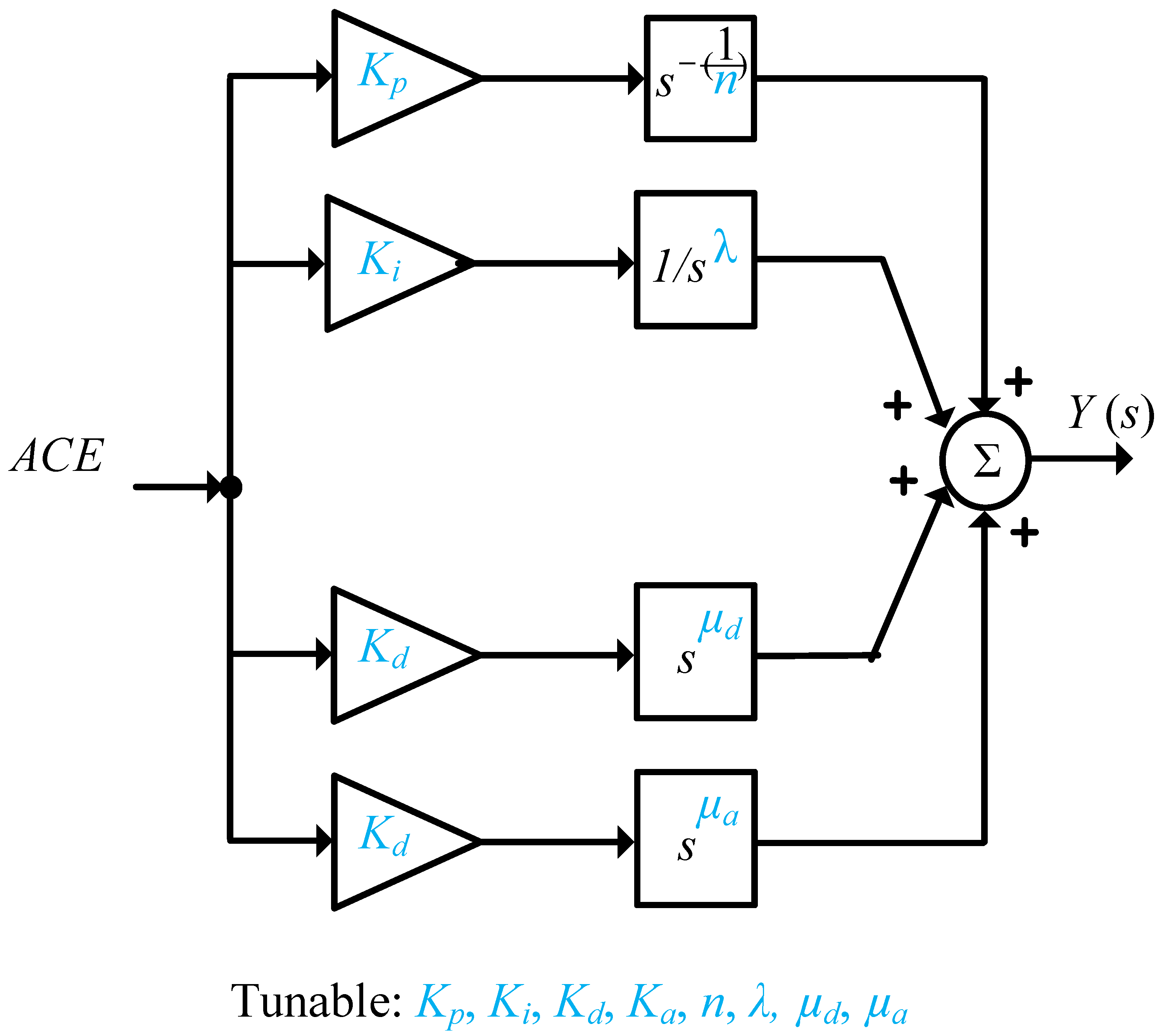
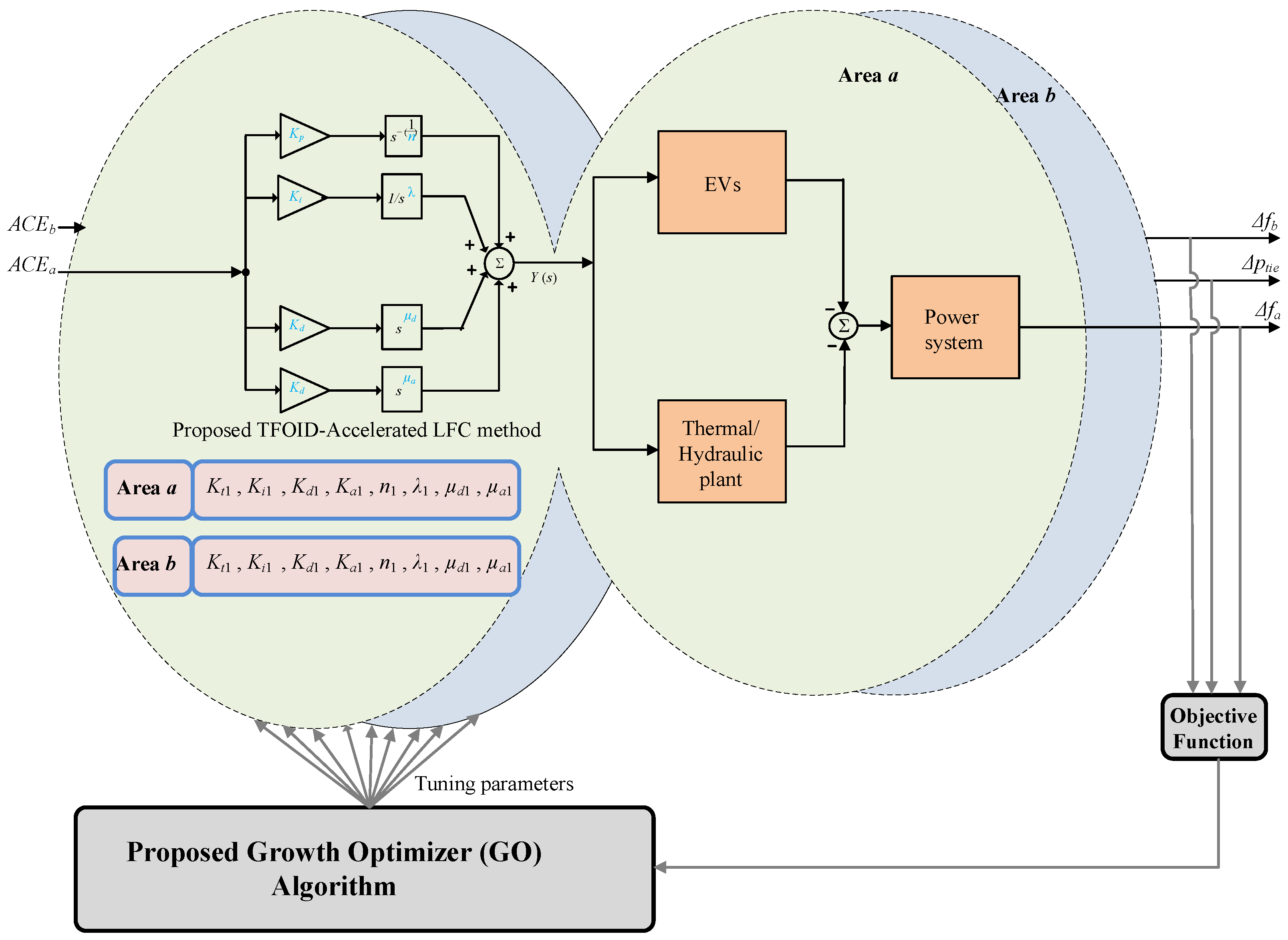
- A new strategy for optimal fractional-order LFC enhancing the resilience of multi-microgrid systems is developed. The method employs a centralized TFOID-Accelerated controller to manage power output from traditional power stations and electric vehicles. The controller’s accelerated derivative structure effectively counters high-frequency disturbances, while its tilt component and fractional integration address low-frequency disturbances.
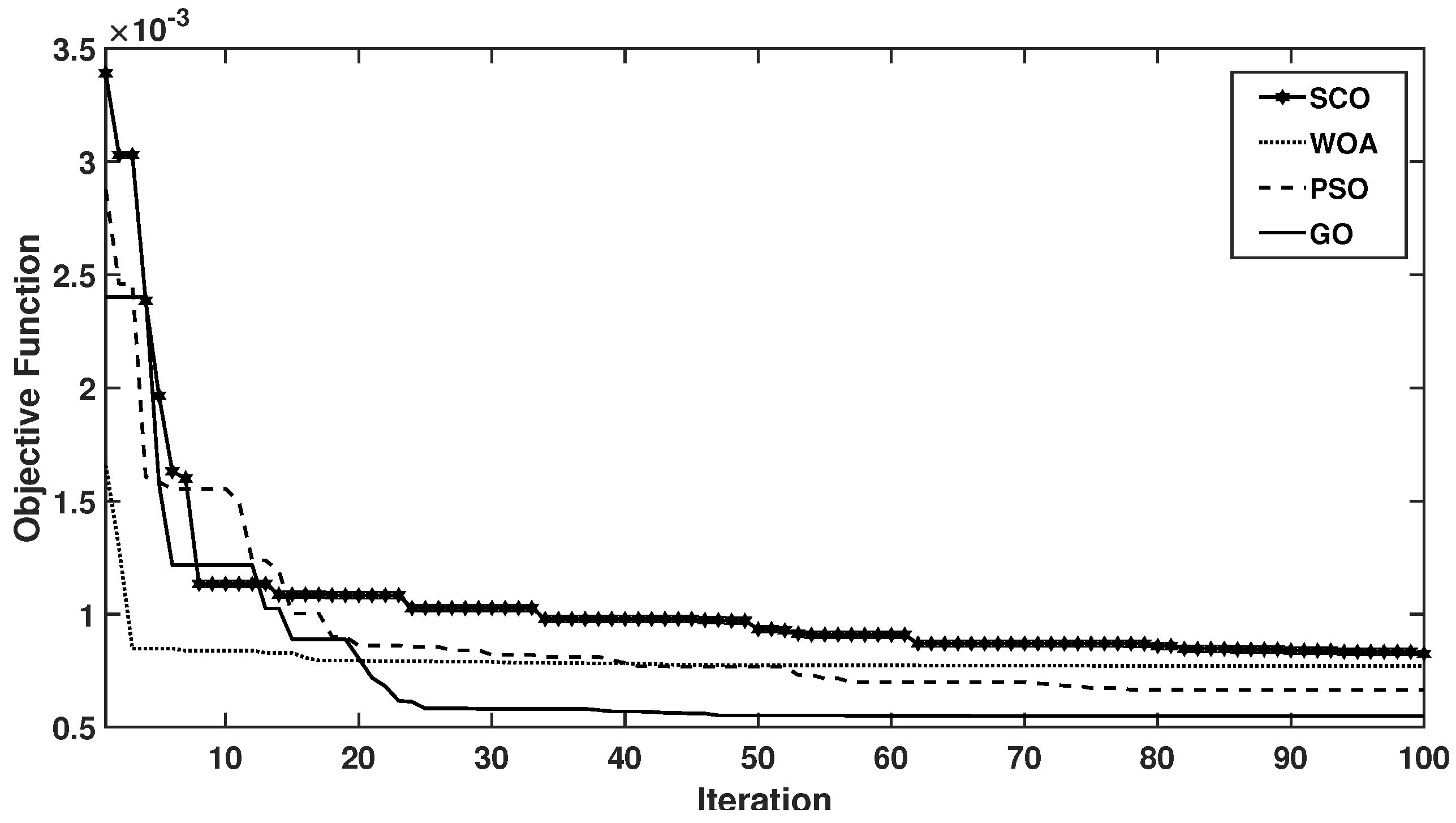
- The GO technique is used to optimize control parameters for proposed controllers across different interconnected multi-MG systems. This optimizer determines the best settings to achieve optimal system response and stability, considering the constraints of various multi-MG systems.
- The suggested approach leverages installed RESs and EV batteries by concurrently designing the proposed coordinated LFC and EV controllers.
- The evaluation of the proposed method’s robustness and effectiveness takes into account a range of anticipated scenarios, RESs, and uncertainties.
- A thorough comparison with controllers from the existing literature demonstrates the superior performance of the proposed controller.

| References | Controllers | Algorithms | Category | Main Characteristics of Category |
|---|---|---|---|---|
| [44,45] | I | ESO with BE, JBO | IOC-based | Easily implementable |
| [21] | I, PI | PSO | single-loop | Low ability to mitigate disturbance |
| [20,46] | PI | HHO, ARO | structure | Possess simple single-loop structure |
| [47,48] | PID | ICA, ABC | Reduced robustness at parametric uncertainty | |
| [19] | Non-linear PI | DO | ||
| [49] | Fuzzy-PIDD2 | GBO | ||
| [50,51] | FOPID | SCA, MDWA | FOC-based | Increased number of tunable parameters |
| [26] | TID | MRFO | single-loop | Higher flexibility than IOC methods |
| [52] | FOPIDF | ICA | structure | Better mitigation of disturbance |
| [31] | iFOI | GWO | Moderate disturbance rejection performance | |
| [30] | FOPIDA | GWO | ||
| [27] | TFOID | AEO, SMA | ||
| [53] | PD-PI | ESMOA | Multi-loop- | Higher number of tunable parameters |
| [54] | PI-PDF | DTBO | based control | Mitigating both high- and low-frequency disturbance |
| [57] | FO-IDF | ICA | structures | Highest in design flexibility |
| [55] | PI-TDF | SSA | Enhanced performance compared to IOC and FOC single-loop methods | |
| [56] | PD-PID | BA | ||
| [42] | FOPI-IDDF | CSA | ||
| [58] | 2DOF PID | TLBO | ||
| [59] | 3DOF TID | SSA | ||
| Proposed | Centralized TFOID-Accelerated | Growth Optimizer (GO) | Single-loop modified FOC | Including tilt component and fractional integration address low-frequency disturbances |
| Including accelerated derivative structure effectively counters high-frequency disturbances | ||||
| Centralized single controller for LFC and EV control | ||||
| Proving better possibility for rejecting disturbances | ||||
| Proposed | Centralized TFOID-Accelerated | Growth Optimizer (GO) | Single-loop modified FOC | Coordinated LFC and EV control in the design process of the optimum controller |
| Applies recently developed powerful Growth Optimizer (GO) algorithm | ||||
| Simultaneous determination of optimized parameter set of controllers in both areas |
1.4. Paper Organization
2. Overall Structure and Model of Studied Power System
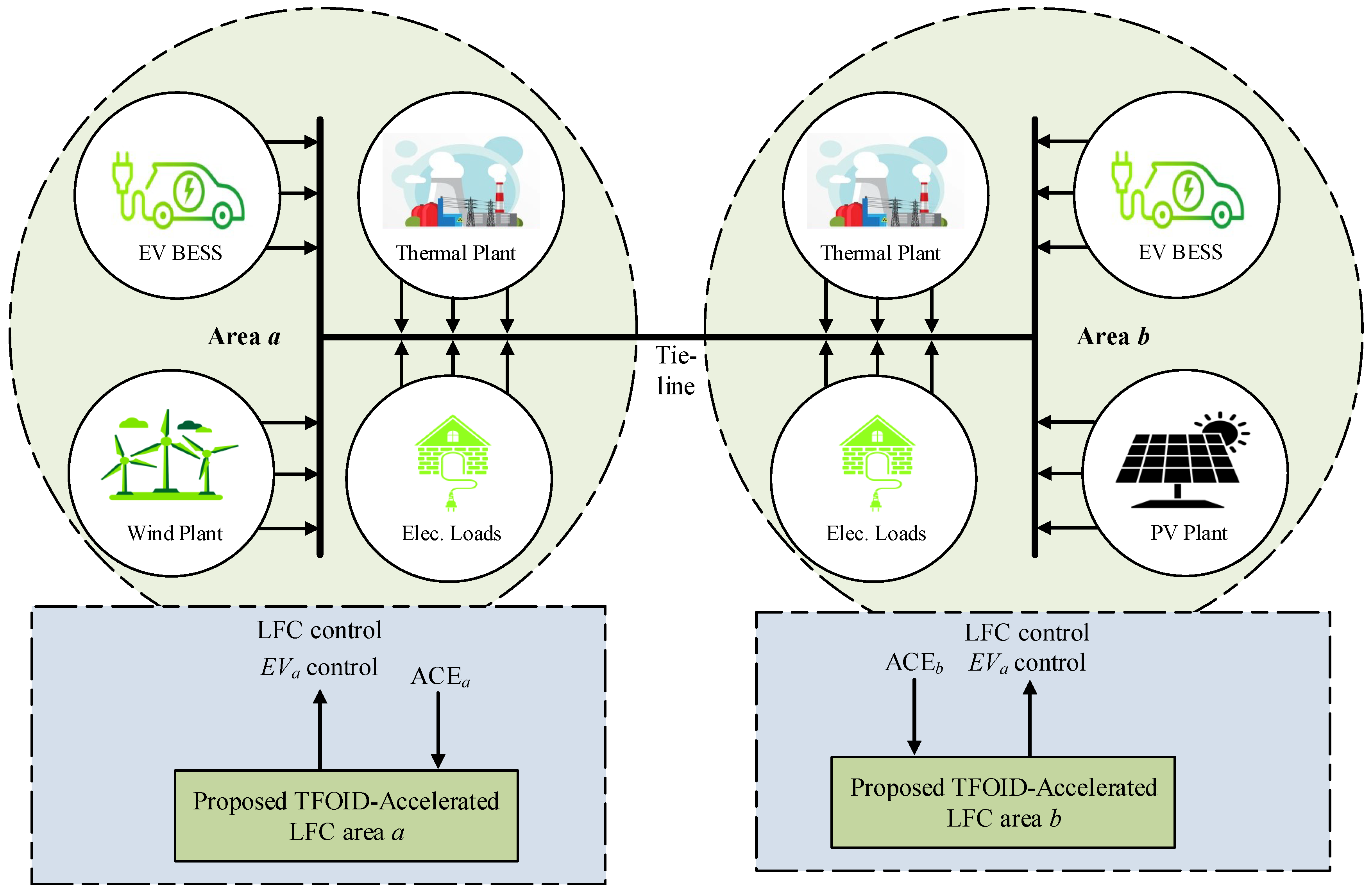
2.1. Overall Structure Description
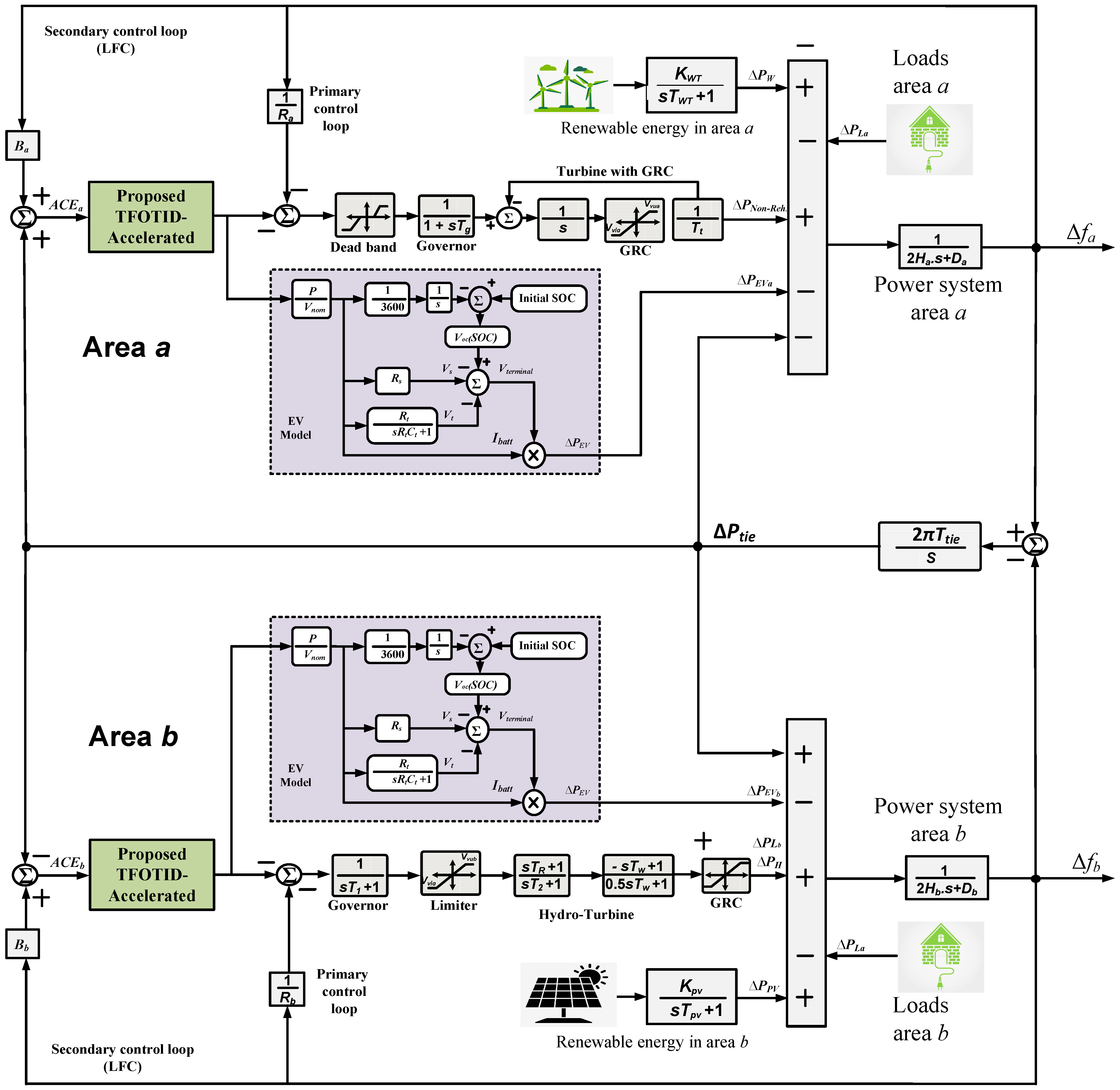
2.2. EV Model Description
2.3. PV Plant Representation
2.4. Wind Plant Representation
2.5. Representations of Thermal and Hydraulic Generators and Grid
2.6. Complete System Representation
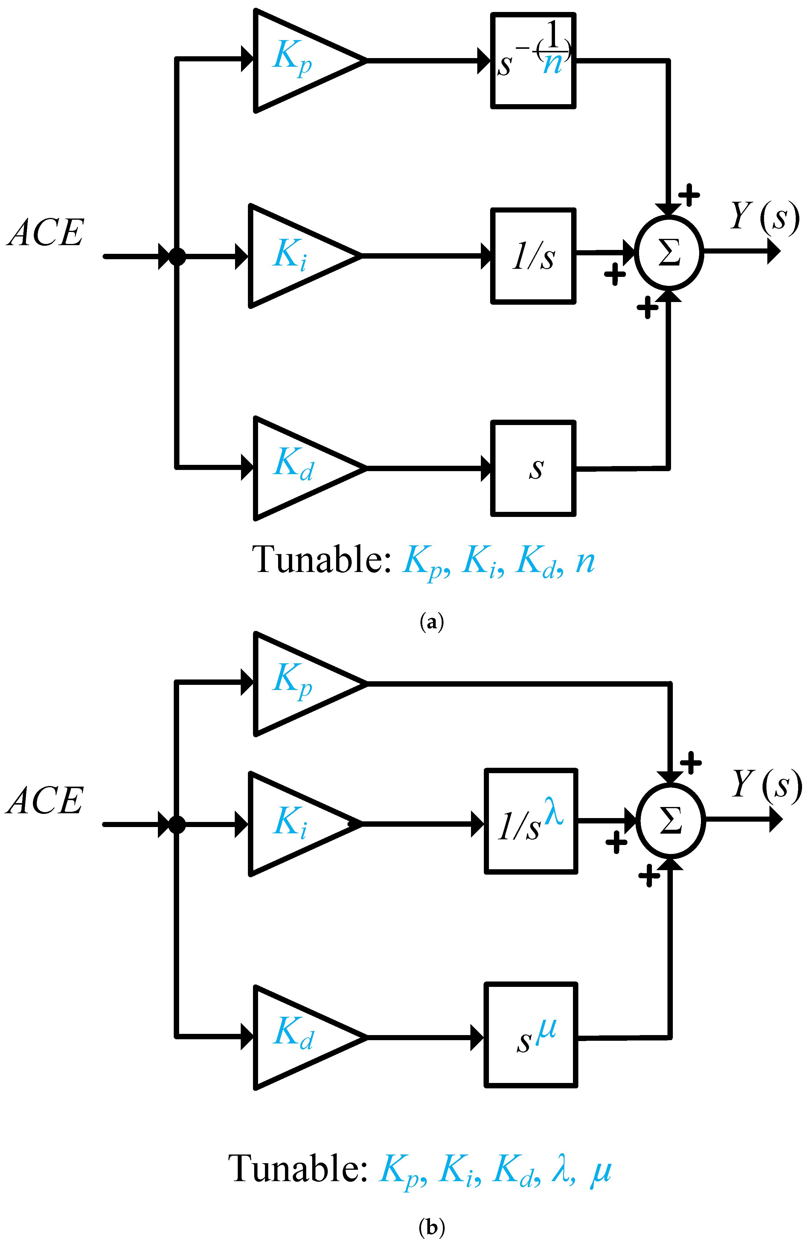
3. Development of Proposed TFOID-Accelerated Controller
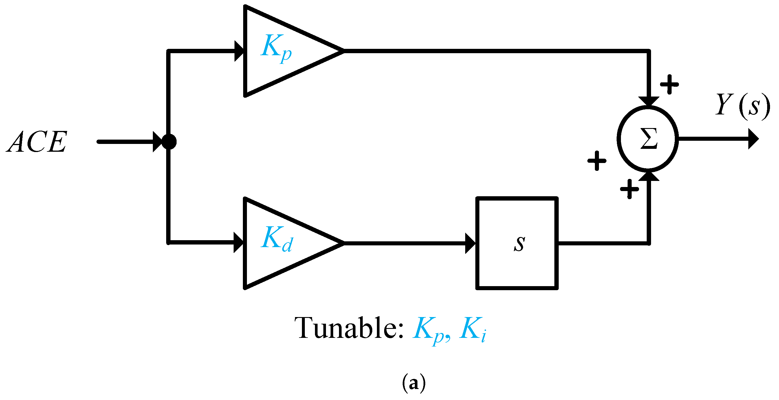
3.1. LFC Based on FOC Method
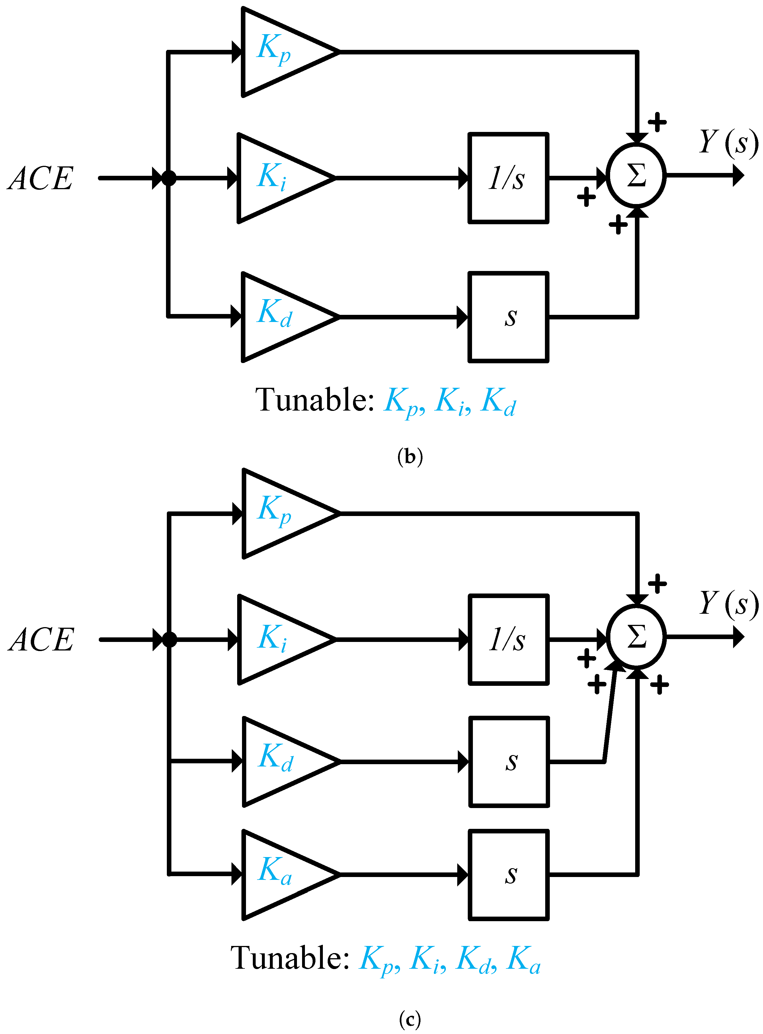
3.2. FOC-Based LFC Representation
3.3. Proposed FOC-Based LFC Using TFOID-Accelerated Controller
4. Proposed Optimal Controller Design
4.1. Growth Optimizer Description and Algorithm
| Algorithm 1 Pseudo-code for proposed parameters tuning based on GO algorithm |
|
4.1.1. Learning Stage
4.1.2. Reflection Stage
4.2. Proposed GO Algorithm-Based TFOID-Accelerated Design
5. Results and Discussion
- Scenario 1: The impact of one-step load pattern (1SLP).
- Scenario 2: The impact of two-step load pattern (2SLP).
- Scenario 3: The impact of multi-load pattern (MLP).
- Scenario 4: The impact of the RESs fluctuations.
- Scenario 5: The impact of high penetration of RESs fluctuations.
- Scenario 6: The impact of parameters uncertainties.
5.1. Scenario 1
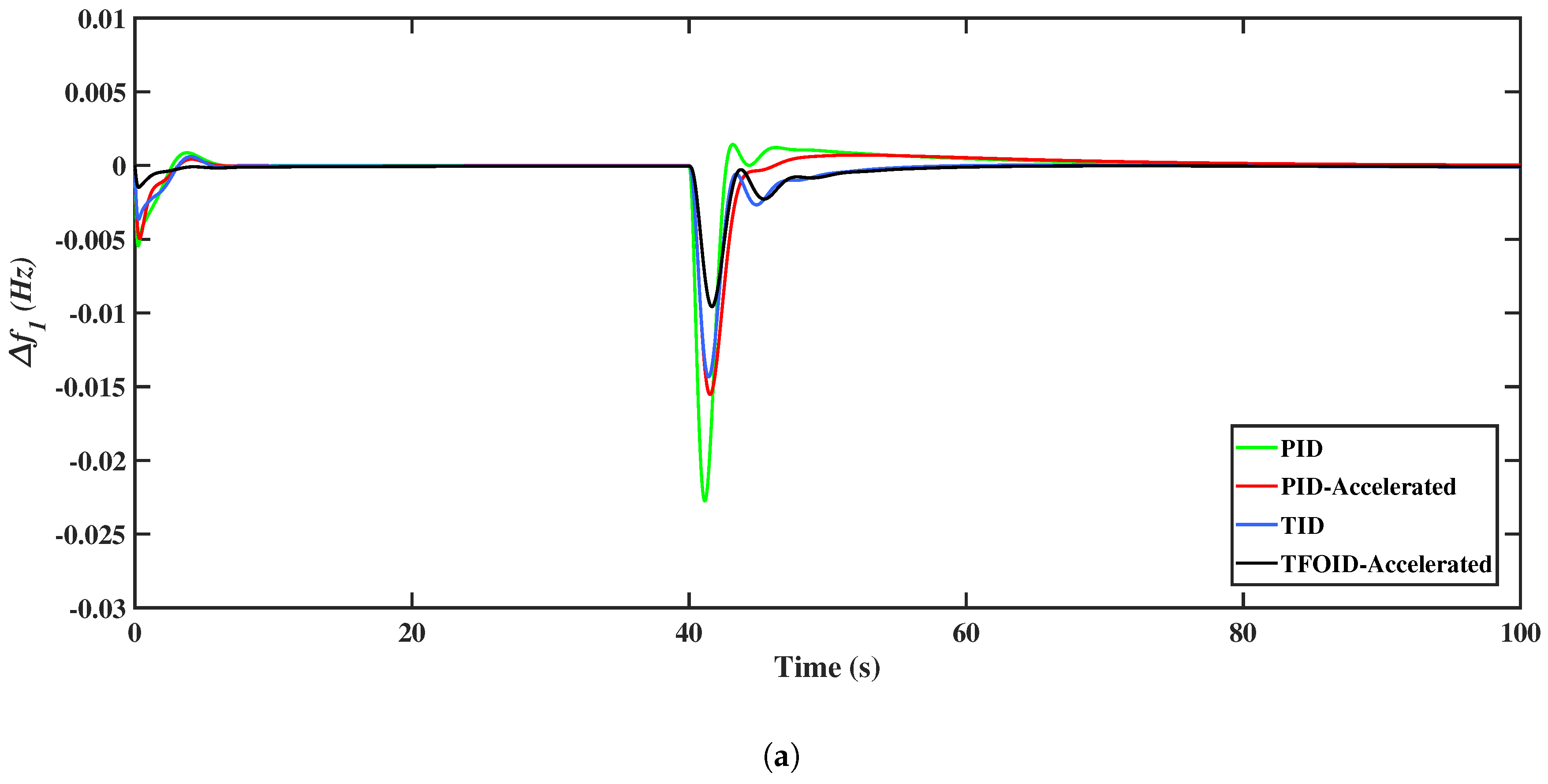
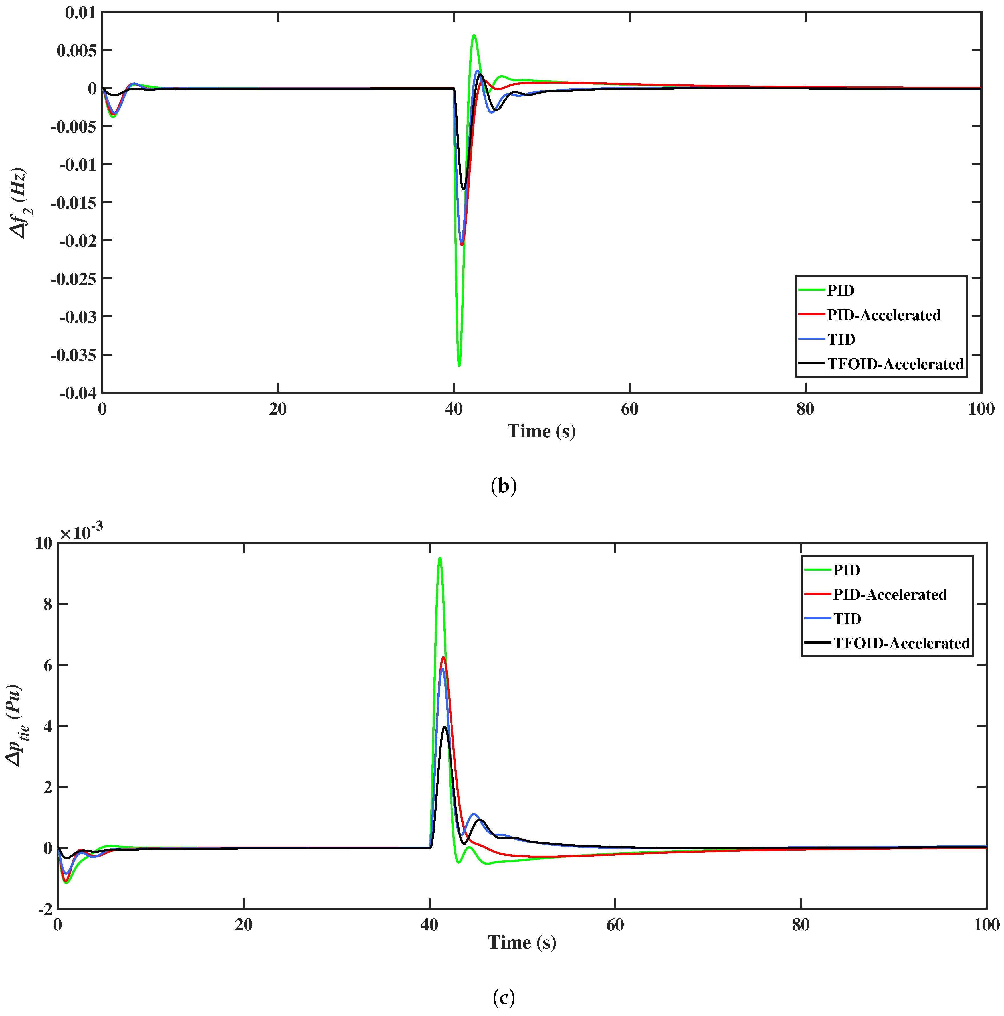
5.2. Scenario 2
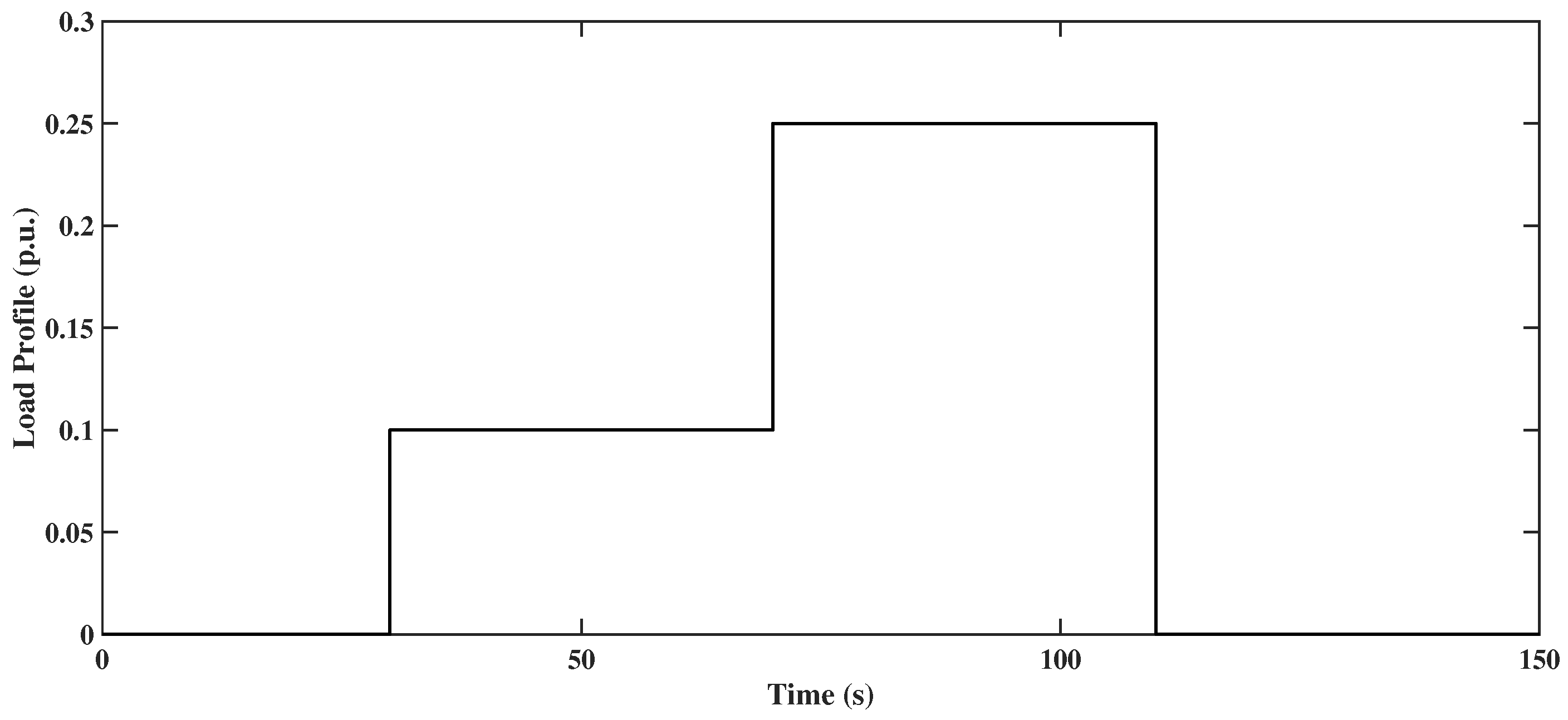
5.3. Scenario 3
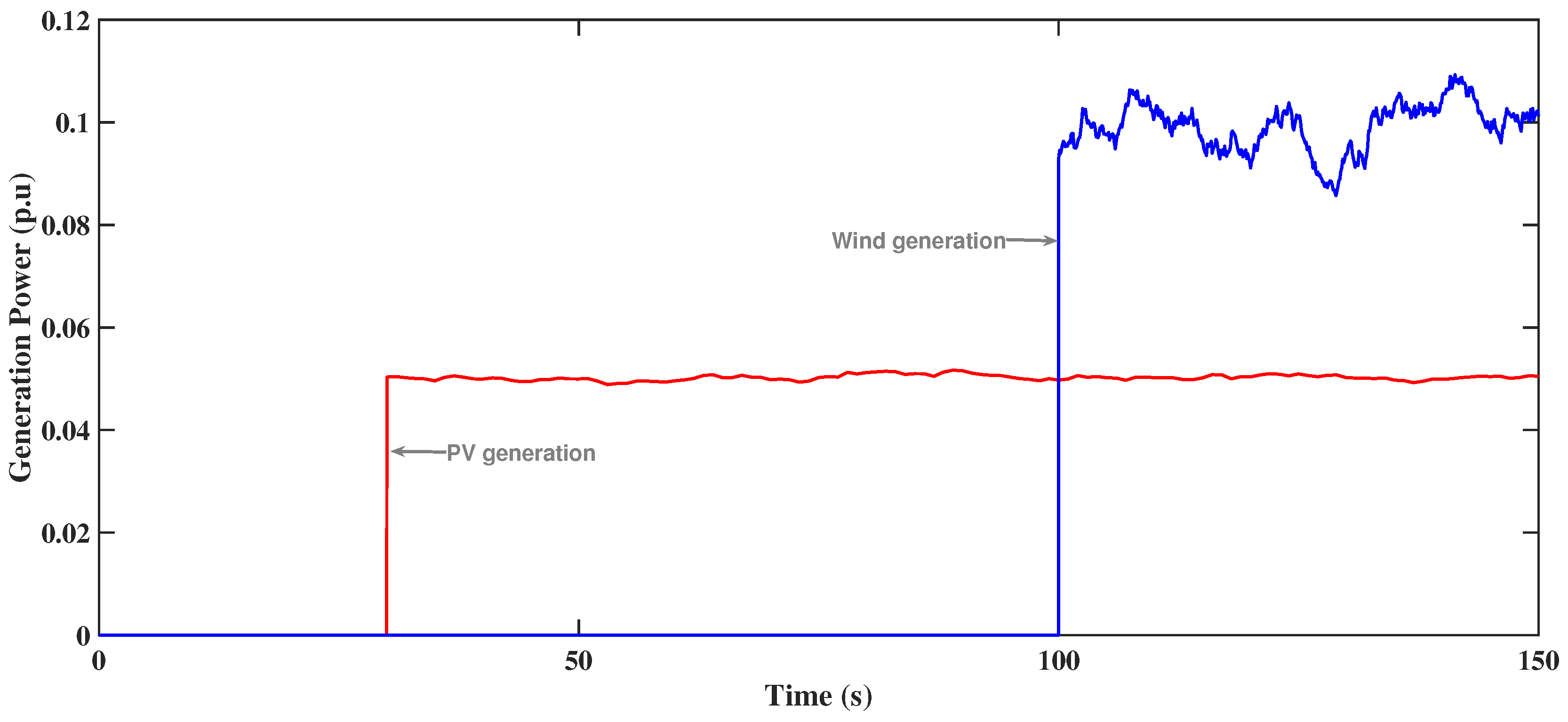
5.4. Scenario 4
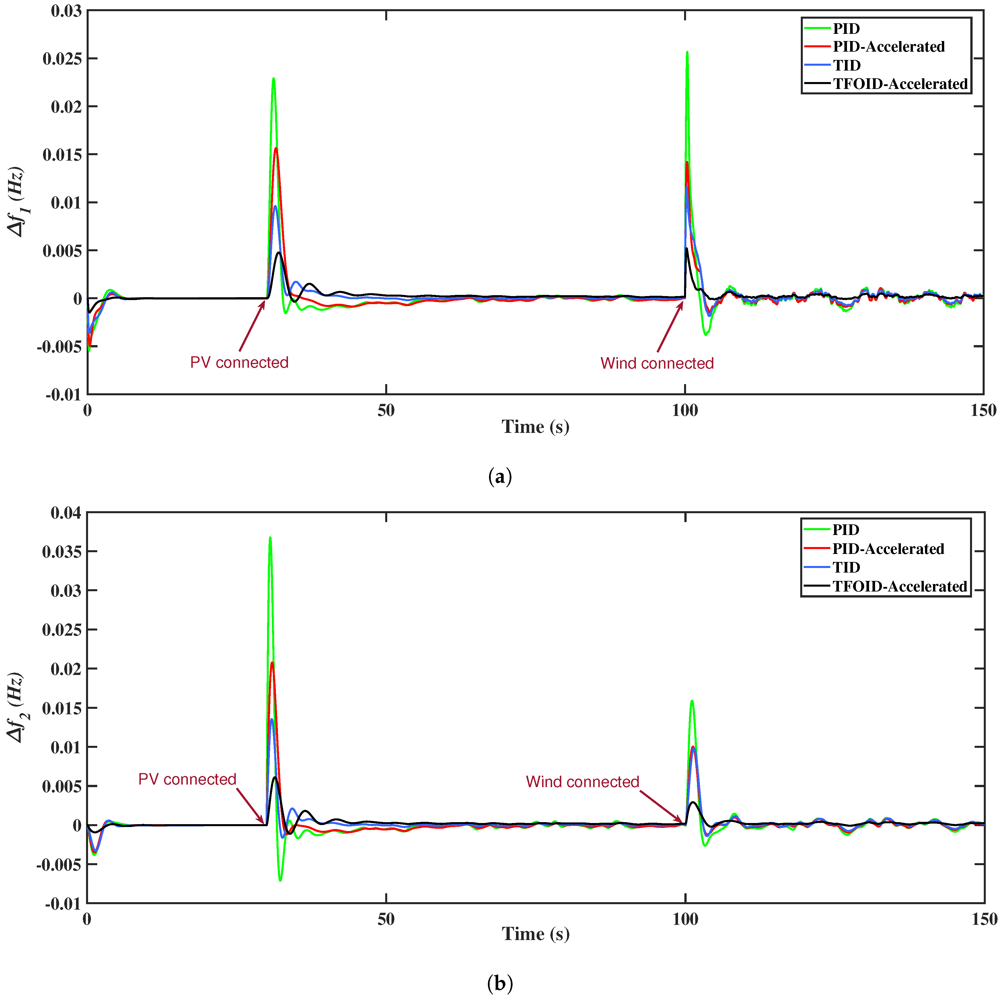
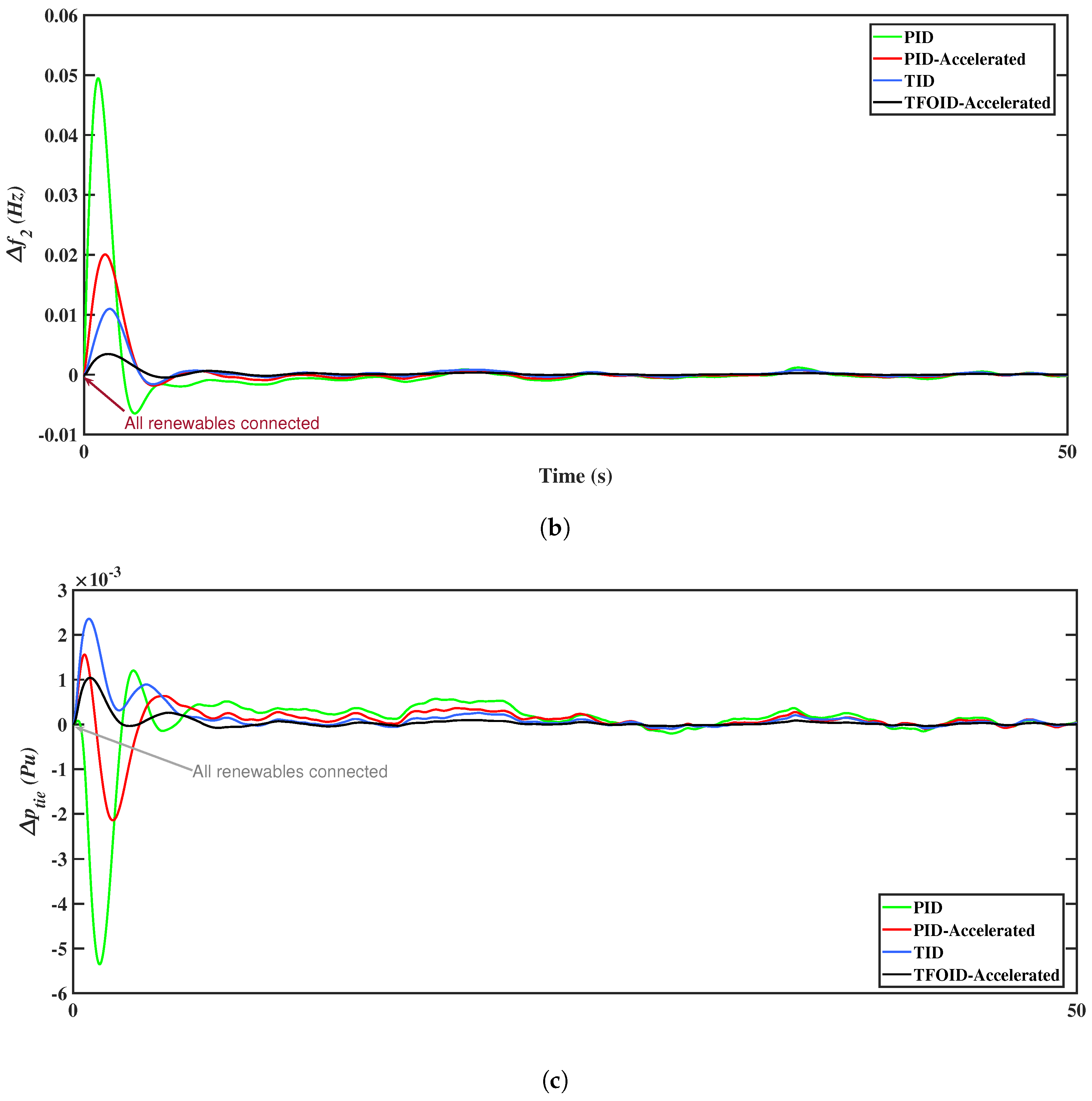
5.5. Scenario 5
5.6. Scenario 6
6. Conclusions
Author Contributions
Funding
Data Availability Statement
Conflicts of Interest
References
- Faheem, M.; Kuusniemi, H.; Eltahawy, B.; Bhutta, M.S.; Raza, B. A lightweight smart contracts framework for blockchain-based secure communication in smart grid applications. IET Gener. Transm. Distrib. 2024, 18, 625–638. [Google Scholar] [CrossRef]
- Das, D.C.; Roy, A.; Sinha, N. GA based frequency controller for solar thermal–diesel–wind hybrid energy generation/energy storage system. Int. J. Electr. Power Energy Syst. 2012, 43, 262–279. [Google Scholar] [CrossRef]
- Zeynali, S.; Rostami, N.; Feyzi, M. Multi-objective optimal short-term planning of renewable distributed generations and capacitor banks in power system considering different uncertainties including plug-in electric vehicles. Int. J. Electr. Power Energy Syst. 2020, 119, 105885. [Google Scholar] [CrossRef]
- Blaabjerg, F.; Yang, Y.; Kim, K.A.; Rodriguez, J. Power Electronics Technology for Large-Scale Renewable Energy Generation. Proc. IEEE 2023, 111, 335–355. [Google Scholar] [CrossRef]
- Zografos, D.; Ghandhari, M. Power system inertia estimation by approaching load power change after a disturbance. In Proceedings of the 2017 IEEE Power & Energy Society General Meeting, Chicago, IL, USA, 16–20 July 2017; pp. 1–5. [Google Scholar] [CrossRef]
- Tielens, P.; Van Hertem, D. The relevance of inertia in power systems. Renew. Sustain. Energy Rev. 2016, 55, 999–1009. [Google Scholar] [CrossRef]
- International Energy Agency. Renewables 2022: Analysis and Forecast to 2027. 2023. Available online: https://www.iea.org/reports/renewables-2022 (accessed on 19 May 2023).
- Smith, C.; Burrows, J.; Scheier, E.; Young, A.; Smith, J.; Young, T.; Gheewala, S.H. Comparative Life Cycle Assessment of a Thai Island’s diesel/PV/wind hybrid microgrid. Renew. Energy 2015, 80, 85–100. [Google Scholar] [CrossRef]
- Tripathi, S.; Singh, V.P.; Kishor, N.; Pandey, A. Load frequency control of power system considering electric Vehicles’ aggregator with communication delay. Int. J. Electr. Power Energy Syst. 2023, 145, 108697. [Google Scholar] [CrossRef]
- Hosseini, S.A. Frequency control using electric vehicles with adaptive latency compensation and variable speed wind turbines using modified virtual inertia controller. Int. J. Electr. Power Energy Syst. 2024, 155, 109535. [Google Scholar] [CrossRef]
- Amir, M.; Zaheeruddin; Haque, A.; Bakhsh, F.I.; Kurukuru, V.S.B.; Sedighizadeh, M. Intelligent energy management scheme-based coordinated control for reducing peak load in grid-connected photovoltaic-powered electric vehicle charging stations. IET Gener. Transm. Distrib. 2023, 18, 1205–1222. [Google Scholar] [CrossRef]
- Liang, J.; Feng, J.; Fang, Z.; Lu, Y.; Yin, G.; Mao, X.; Wu, J.; Wang, F. An Energy-Oriented Torque-Vector Control Framework for Distributed Drive Electric Vehicles. IEEE Trans. Transp. Electrif. 2023, 9, 4014–4031. [Google Scholar] [CrossRef]
- Liang, J.; Wang, F.; Feng, J.; Zhao, M.; Fang, R.; Pi, D.; Yin, G. A Hierarchical Control of Independently Driven Electric Vehicles Considering Handling Stability and Energy Conservation. IEEE Trans. Intell. Veh. 2024, 9, 738–751. [Google Scholar] [CrossRef]
- Choudhary, R.; Rai, J.; Arya, Y. FOPTID1 controller with capacitive energy storage for AGC performance enrichment of multi-source electric power systems. Electr. Power Syst. Res. 2023, 221, 109450. [Google Scholar] [CrossRef]
- Saikia, L.; Nanda, J.; Mishra, S. Performance comparison of several classical controllers in AGC for multi-area interconnected thermal system. Int. J. Electr. Power Energy Syst. 2011, 33, 394–401. [Google Scholar] [CrossRef]
- Raju, M.; Saikia, L.; Sinha, N. Automatic generation control of a multi-area system using ant lion optimizer algorithm based PID plus second order derivative controller. Int. J. Electr. Power Energy Syst. 2016, 80, 52–63. [Google Scholar] [CrossRef]
- Ali, E.; Abd-Elazim, S. Bacteria foraging optimization algorithm based load frequency controller for interconnected power system. Int. J. Electr. Power Energy Syst. 2011, 33, 633–638. [Google Scholar] [CrossRef]
- Hasan, N.; Alsaidan, I.; Sajid, M.; Khatoon, S.; Farooq, S. Robust self tuned AGC controller for wind energy penetrated power system. Ain Shams Eng. J. 2022, 13, 101663. [Google Scholar] [CrossRef]
- Almasoudi, F.; Bakeer, A.; Magdy, G.; Alatawi, K.; Shabib, G.; Lakhouit, A.; Alomrani, S. Nonlinear coordination strategy between renewable energy sources and fuel cells for frequency regulation of hybrid power systems. Ain Shams Eng. J. 2023, 15, 102399. [Google Scholar] [CrossRef]
- Khalil, A.; Boghdady, T.; Alham, M.; Ibrahim, D. Enhancing the conventional controllers for load frequency control of isolated microgrids using proposed multi-objective formulation via artificial rabbits optimization algorithm. IEEE Access 2023, 11, 3472–3493. [Google Scholar] [CrossRef]
- Bakeer, M.; Magdy, G.; Bakeer, A.; Aly, M. Resilient virtual synchronous generator approach using DC-link capacitor energy for frequency support of interconnected renewable power systems. J. Energy Storage 2023, 65, 107230. [Google Scholar] [CrossRef]
- Taher, S.; Fini, M.; Aliabadi, S. Fractional order PID controller design for LFC in electric power systems using imperialist competitive algorithm. Ain Shams Eng. J. 2014, 5, 121–135. [Google Scholar] [CrossRef]
- Khamari, D.; Sahu, R.; Gorripotu, T.; Panda, S. Automatic generation control of power system in deregulated environment using hybrid TLBO and pattern search technique. Ain Shams Eng. J. 2020, 11, 553–573. [Google Scholar] [CrossRef]
- Guha, D.; Roy, P.; Banerjee, S. Maiden application of SSA-optimised CC-TID controller for load frequency control of power systems. IET Gener. Transm. Distrib. 2019, 13, 1110–1120. [Google Scholar] [CrossRef]
- Elmelegi, A.; Mohamed, E.; Aly, M.; Ahmed, E.; Mohamed, A.A.; Elbaksawi, O. Optimized tilt fractional order cooperative controllers for preserving frequency stability in renewable energy-based power systems. IEEE Access 2021, 9, 8261–8277. [Google Scholar] [CrossRef]
- Mohamed, E.; Ahmed, E.; Elmelegi, A.; Aly, M.; Elbaksawi, O.; Mohamed, A.A. An optimized hybrid fractional order controller for frequency regulation in multi-area power systems. IEEE Access 2020, 8, 213899–213915. [Google Scholar] [CrossRef]
- Ahmed, E.; Mohamed, E.; Elmelegi, A.; Aly, M.; Elbaksawi, O. Optimum modified fractional order controller for future electric vehicles and renewable energy-based interconnected power systems. IEEE Access 2021, 9, 29993–30010. [Google Scholar] [CrossRef]
- Khadanga, R.; Kumar, A.; Panda, S. A modified grey wolf optimization with cuckoo search algorithm for load frequency controller design of hybrid power system. Appl. Soft Comput. 2022, 124, 109011. [Google Scholar] [CrossRef]
- Singh, K.; Arya, Y. Jaya-ITDF control strategy-based frequency regulation of multimicrogrid utilizing energy stored in high-voltage direct current-link capacitors. Soft Comput. 2023, 27, 5951–5970. [Google Scholar] [CrossRef]
- Almasoudi, F.; Magdy, G.; Bakeer, A.; Alatawi, K.; Rihan, M. A new load frequency control technique for hybrid maritime microgrids: Sophisticated structure of fractional-order PIDA controller. Fractal Fract. 2023, 7, 435. [Google Scholar] [CrossRef]
- Zaid, S.; Bakeer, A.; Magdy, G.; Albalawi, H.; Kassem, A.; El-Shimy, M.; AbdelMeguid, H.; Manqarah, B. A new intelligent fractional-order load frequency control for interconnected modern power systems with virtual inertia control. Fractal Fract. 2023, 7, 62. [Google Scholar] [CrossRef]
- Kumari, S.; Shankar, G. Novel application of integral-tilt-derivative controller for performance evaluation of load frequency control of interconnected power system. IET Gener. Transm. Distrib. 2018, 12, 3550–3560. [Google Scholar] [CrossRef]
- Barakat, M. Novel chaos game optimization tuned-fractional-order PID fractional-order PI controller for load–frequency control of interconnected power systems. Prot. Control. Mod. Power Syst. 2022, 7. [Google Scholar] [CrossRef]
- Prakash, A.; Kumar, K.; Parida, S. PIDF(1+FOD) controller for load frequency control with SSSC and AC–DC tie-line in deregulated environment. IET Gener. Transm. Distrib. 2020, 14, 2751–2762. [Google Scholar] [CrossRef]
- Khokhar, B.; Dahiya, S.; Parmar, K. A novel fractional order proportional integral derivative plus second-order derivative controller for load frequency control. Int. J. Sustain. Energy 2020, 40, 235–252. [Google Scholar] [CrossRef]
- Arya, Y. AGC of PV-thermal and hydro-thermal power systems using CES and a new multi-stage FPIDF-(1PI) controller. Renew. Energy 2019, 134, 796–806. [Google Scholar] [CrossRef]
- Guha, D.; Roy, P.; Banerjee, S. Disturbance observer aided optimised fractional-order three-degree-of-freedom tilt-integral-derivative controller for load frequency control of power systems. IET Gener. Transm. Distrib. 2020, 15, 716–736. [Google Scholar] [CrossRef]
- Chinta, D.; Jatoth, R.; Biswal, M. Power system frequency profile improvement using satin bowerbird optimized tilt fractional cascade controller with reduced data based cost function. J. Eng. Res. 2023, 11, 100116. [Google Scholar] [CrossRef]
- Jena, N.; Sahoo, S.; Sahu, B.; Naik, A.; Bajaj, M.; Misak, S.; Blazek, V.; Prokop, L. Impact of a redox flow battery on the frequency stability of a five-area system integrated with renewable sources. Energies 2023, 16, 5540. [Google Scholar] [CrossRef]
- Ahmed, N.; Ebeed, M.; Magdy, G.; Sayed, K.; Gamoura, S.; Metwally, A.; Mahmoud, A.A. A new optimized FOPIDA-FOIDN controller for the frequency regulation of hybrid multi-area interconnected microgrids. Fractal Fract. 2023, 7, 666. [Google Scholar] [CrossRef]
- Rangi, S.; Jain, S.; Arya, Y. scpSSA/scp-optimized cascade scpoptimal-PIDN/scp controller for multi-area power system with scpRFB/scp under deregulated environment. Optim. Control. Appl. Methods 2022, 44, 1972–1994. [Google Scholar] [CrossRef]
- Babu, N.; Bhagat, S.; Chiranjeevi, T.; Pushkarna, M.; Saha, A.; Kotb, H.; AboRas, K.; Alsaif, F.; Alsulamy, S.; Ghadi, Y.; et al. Frequency control of a realistic dish stirling solar thermal system and accurate HVDC models using a cascaded FOPI-IDDN-based crow search algorithm. Int. J. Energy Res. 2023, 2023, 9976375. [Google Scholar] [CrossRef]
- Noman, A.M.; Aly, M.; Alqahtani, M.H.; Almutairi, S.Z.; Aljumah, A.S.; Ebeed, M.; Mohamed, E.A. Optimum Fractional Tilt Based Cascaded Frequency Stabilization with MLC Algorithm for Multi-Microgrid Assimilating Electric Vehicles. Fractal Fract. 2024, 8, 132. [Google Scholar] [CrossRef]
- Dahab, Y.A.; Abubakr, H.; Mohamed, T.H. Adaptive Load Frequency Control of Power Systems Using Electro-Search Optimization Supported by the Balloon Effect. IEEE Access 2020, 8, 7408–7422. [Google Scholar] [CrossRef]
- Ewais, A.M.; Elnoby, A.M.; Mohamed, T.H.; Mahmoud, M.M.; Qudaih, Y.; Hassan, A.M. Adaptive frequency control in smart microgrid using controlled loads supported by real-time implementation. PLoS ONE 2023, 18, e0283561. [Google Scholar] [CrossRef]
- Yousri, D.; Babu, T.S.; Fathy, A. Recent methodology based Harris Hawks optimizer for designing load frequency control incorporated in multi-interconnected renewable energy plants. Sustain. Energy Grids Netw. 2020, 22, 100352. [Google Scholar] [CrossRef]
- Shabani, H.; Vahidi, B.; Ebrahimpour, M. A robust PID controller based on imperialist competitive algorithm for load-frequency control of power systems. ISA Trans. 2013, 52, 88–95. [Google Scholar] [CrossRef]
- El Yakine Kouba, N.; Menaa, M.; Hasni, M.; Boudour, M. Optimal load frequency control based on artificial bee colony optimization applied to single, two and multi-area interconnected power systems. In Proceedings of the 2015 3rd International Conference on Control, Engineering & Information Technology (CEIT), Tlemcen, Algeria, 25–27 May 2015; pp. 1–6. [Google Scholar] [CrossRef]
- AboRas, K.M.; Ragab, M.; Shouran, M.; Alghamdi, S.; Kotb, H. Voltage and frequency regulation in smart grids via a unique Fuzzy PIDD2 controller optimized by Gradient-Based Optimization algorithm. Energy Rep. 2023, 9, 1201–1235. [Google Scholar] [CrossRef]
- Fathy, A.; Alharbi, A.G. Recent Approach Based Movable Damped Wave Algorithm for Designing Fractional-Order PID Load Frequency Control Installed in Multi-Interconnected Plants with Renewable Energy. IEEE Access 2021, 9, 71072–71089. [Google Scholar] [CrossRef]
- Ayas, M.S.; Sahin, E. FOPID controller with fractional filter for an automatic voltage regulator. Comput. Electr. Eng. 2021, 90, 106895. [Google Scholar] [CrossRef]
- Zaheeruddin; Singh, K. Load frequency regulation by de-loaded tidal turbine power plant units using fractional fuzzy based PID droop controller. Appl. Soft Comput. 2020, 92, 106338. [Google Scholar] [CrossRef]
- Abid, S.; El-Rifaie, A.M.; Elshahed, M.; Ginidi, A.R.; Shaheen, A.M.; Moustafa, G.; Tolba, M.A. Development of Slime Mold Optimizer with Application for Tuning Cascaded PD-PI Controller to Enhance Frequency Stability in Power Systems. Mathematics 2023, 11, 1796. [Google Scholar] [CrossRef]
- Zhang, G.; Daraz, A.; Khan, I.A.; Basit, A.; Khan, M.I.; Ullah, M. Driver Training Based Optimized Fractional Order PI-PDF Controller for Frequency Stabilization of Diverse Hybrid Power System. Fractal Fract. 2023, 7, 315. [Google Scholar] [CrossRef]
- Malik, S.; Suhag, S. A Novel SSA Tuned PI-TDF Control Scheme for Mitigation of Frequency Excursions in Hybrid Power System. Smart Sci. 2020, 8, 202–218. [Google Scholar] [CrossRef]
- Dash, P.; Saikia, L.; Sinha, N. Automatic generation control of multi area thermal system using Bat algorithm optimized PD–PID cascade controller. Int. J. Electr. Power Energy Syst. 2015, 68, 364–372. [Google Scholar] [CrossRef]
- Arya, Y.; Kumar, N.; Dahiya, P.; Sharma, G.; Çelik, E.; Dhundhara, S.; Sharma, M. Cascade-IλDμN controller design for AGC of thermal and hydro-thermal power systems integrated with renewable energy sources. IET Renew. Power Gener. 2021, 15, 504–520. [Google Scholar] [CrossRef]
- Sahu, R.; Panda, S.; Rout, U.K.; Sahoo, D. Teaching learning based optimization algorithm for automatic generation control of power system using 2-DOF PID controller. Int. J. Electr. Power Energy Syst. 2016, 77, 287–301. [Google Scholar] [CrossRef]
- Oshnoei, S.; Aghamohammadi, M.; Oshnoei, S.; Oshnoei, A.; Mohammadi-Ivatloo, B. Provision of Frequency Stability of an Islanded Microgrid Using a Novel Virtual Inertia Control and a Fractional Order Cascade Controller. Energies 2021, 14, 4152. [Google Scholar] [CrossRef]
- El-Sousy, F.F.M.; Aly, M.; Alqahtani, M.H.; Aljumah, A.S.; Almutairi, S.Z.; Mohamed, E.A. New Cascaded 1+PII2D/FOPID Load Frequency Controller for Modern Power Grids including Superconducting Magnetic Energy Storage and Renewable Energy. Fractal Fract. 2023, 7, 672. [Google Scholar] [CrossRef]
- Micev, M.; Ćalasan, M.; Oliva, D. Fractional Order PID Controller Design for an AVR System Using Chaotic Yellow Saddle Goatfish Algorithm. Mathematics 2020, 8, 1182. [Google Scholar] [CrossRef]
- Dulf, E.H. Simplified Fractional Order Controller Design Algorithm. Mathematics 2019, 7, 1166. [Google Scholar] [CrossRef]
- Motorga, R.; Mureșan, V.; Ungureșan, M.L.; Abrudean, M.; Vălean, H.; Clitan, I. Artificial Intelligence in Fractional-Order Systems Approximation with High Performances: Application in Modelling of an Isotopic Separation Process. Mathematics 2022, 10, 1459. [Google Scholar] [CrossRef]
- Zhang, Q.; Gao, H.; Zhan, Z.H.; Li, J.; Zhang, H. Growth Optimizer: A powerful metaheuristic algorithm for solving continuous and discrete global optimization problems. Knowl.-Based Syst. 2023, 261, 110206. [Google Scholar] [CrossRef]
- Fatani, A.; Dahou, A.; Abd Elaziz, M.; Al-qaness, M.A.A.; Lu, S.; Alfadhli, S.A.; Alresheedi, S.S. Enhancing Intrusion Detection Systems for IoT and Cloud Environments Using a Growth Optimizer Algorithm and Conventional Neural Networks. Sensors 2023, 23, 4430. [Google Scholar] [CrossRef] [PubMed]
- Aribia, H.B.; El-Rifaie, A.M.; Tolba, M.A.; Shaheen, A.; Moustafa, G.; Elsayed, F.; Elshahed, M. Growth Optimizer for Parameter Identification of Solar Photovoltaic Cells and Modules. Sustainability 2023, 15, 7896. [Google Scholar] [CrossRef]


| Parameters | Symbols | Area a | Area b |
|---|---|---|---|
| Nominal power system size | (MW) | 1200 | 1200 |
| Droop gain | (Hz/MW) | 2.4 | 2.4 |
| Frequency bias | (MW/Hz) | 0.4249 | 0.4249 |
| Valve gate limit (minimum) | (p.u.MW) | 0.5 | 0.5 |
| Valve gate limit (maximum) | (p.u.MW) | 0.5 | 0.5 |
| Thermal governor time constant | (s) | 0.08 | - |
| Thermal turbine time constant | (s) | 0.3 | - |
| Hydraulic governor time constant | (s) | - | 41.6 |
| Hydraulic transient droop time constant | (s) | - | 0.513 |
| Hydraulic governor reset times | (s) | - | 9.6 |
| Water starting time of hydraulic turbines | (s) | - | 1 |
| Area’s inertia constant | (p.u.s) | 0.0833 | 0.0833 |
| Area’s damping coefficient | (p.u./Hz) | 0.00833 | 0.00833 |
| PV transfer function time constant | (s) | - | 1.3 |
| PV transfer function gain | - | 1 | |
| Wind transfer function time constant | (s) | 1.5 | - |
| Wind transfer function gain | 1 | - | |
| EV numbers in each area | - | 150,000 | 150,000 |
| EV participation | - | 5% | 5% |
| Battery state of charges | SOC | 95% | 95% |
| Controller | Area | n | ||||||||
|---|---|---|---|---|---|---|---|---|---|---|
| PID | Area-a | 4.9765 | 4.8871 | 4.3139 | ― | ― | ― | ― | ― | ― |
| Area-b | 4.3636 | 3.4465 | 1.2884 | ― | ― | ― | ― | ― | ― | |
| PID-Accelerated | Area-a | 3.0992 | 3.9542 | 1.0558 | ― | 2.0205 | ― | ― | ― | 1.556 |
| Area-b | 3.9701 | 2.9021 | 1.9667 | ― | 1.3563 | ― | ― | ― | 1.238 | |
| TID | Area-a | ― | 2.5674 | 3.9984 | 1.8184 | ― | 4.955 | ― | ― | ― |
| Area-b | ― | 1.1892 | 1.9497 | 2.9809 | ― | 4.961 | ― | ― | ― | |
| TFOID-Accelerated | Area-a | ― | 4.8906 | 4.7948 | 4.0327 | 2.3681 | 2.631 | 0.923 | 0.416 | 1.271 |
| Area-b | ― | 3.4132 | 3.2288 | 4.2643 | 2.1538 | 3.028 | 0.499 | 0.723 | 1.682 |
| CASE 1 | PID | 0.00086 | 0.0054 | 17.11 | 0.00051 | 0.0038 | 21.45 | 0.00005 | 0.0011 | 18.32 |
| TID | 0.00043 | 0.0049 | 16.12 | 0.00055 | 0.0034 | 18.22 | - | 0.0010 | 16.89 | |
| FOTID | 0.00059 | 0.0036 | 14.12 | 0.00054 | 0.0032 | 15.14 | - | 0.00084 | 14.75 | |
| TFOID-Accelerated | - | 0.0014 | 10.42 | 0.00012 | 0.00092 | 13.02 | - | 0.00035 | 12.81 | |
| CASE 2 40 s | PID | 0.0012 | 0.022 | 57.99 | 0.0066 | 0.036 | 56.43 | 0.0093 | 0.00048 | >100 s |
| TID | 0.00056 | 0.016 | 50.13 | 0.00086 | 0.022 | 52.78 | 0.0061 | 0.00027 | >100 s | |
| FOTID | - | 0.014 | 38.65 | 0.0019 | 0.021 | 38.76 | 0.0.0056 | - | >100 s | |
| TFOID-Accelerated | 0.00038 | 0.0091 | 37.98 | 0.0018 | 0.011 | 37.96 | 0.0038 | 0.00019 | 49.01 | |
| CASE 3 30 s | PID | 0.0045 | 0.027 | 51.76 | 0.0026 | 0.016 | 51.52 | 0.00028 | 0.0055 | 50.22 |
| TID | 0.0025 | 0.021 | 49.53 | 0.0024 | 0.014 | 49.53 | 0.00012 | 0.0041 | 48.40 | |
| FOTID | 0.0023 | 0.013 | 45.78 | 0.0022 | 0.013 | 45.76 | 0.00009 | 0.0026 | 43.19 | |
| TFOID-Accelerated | 0.00023 | 0.0041 | 38.54 | 0.00041 | 0.0029 | 41.11 | 0.00002 | 0.0011 | 39.21 | |
| CASE 4 30 s | PID | 0.022 | 0.0014 | Osc. | 0.036 | 0.0071 | Osc. | 0.00044 | 0.0095 | Osc. |
| TID | 0.015 | 0.00079 | Osc. | 0.021 | 0.00086 | Osc. | 0.00028 | 0.0059 | Osc. | |
| FOTID | 0.0092 | 0.00019 | Osc. | 0.013 | 0.0016 | Osc. | 0.00017 | 0.0039 | Osc. | |
| TFOID-Accelerated | 0.0042 | 0.00024 | Osc. | 0.0053 | 0.00083 | Osc. | 0.00002 | 0.0019 | Osc. | |
| CASE 5 | PID | 0.03525 | 0.00445 | Osc. | 0.04935 | 0.00617 | Osc. | 0.00116 | 0.00532 | Osc. |
| TID | 0.01913 | - | Osc. | 0.02931 | 0.00201 | Osc. | 0.00081 | 0.00469 | Osc. | |
| FOTID | 0.01464 | - | Osc. | 0.0218 | 0.00145 | Osc. | 0.00058 | 0.00221 | Osc. | |
| TFOID-Accelerated | 0.00521 | - | Osc. | 0.00788 | 0.00106 | Osc. | 0.00055 | 0.00158 | Osc. | |
| Parameter | Change | Controller | |||||||||
|---|---|---|---|---|---|---|---|---|---|---|---|
| MO | MU | ST | MO | MU | ST | MO | MU | ST | |||
| +50% | PID | 0.00096 | 0.00622 | 20.19 | 0.00074 | 0.00409 | 19.17 | 0.00004 | 0.00131 | 23.85 | |
| TID | 0.00068 | 0.00565 | 18.46 | 0.00066 | 0.00371 | 16.52 | 0.00001 | 0.00125 | 22.31 | ||
| FOTID | 0.00051 | 0.00422 | 14.32 | 0.00078 | 0.0034 | 14.97 | − | 0.00095 | 18.53 | ||
| FOTIDA | 0.00010 | 0.00179 | 12.12 | 0.00016 | 0.00097 | 14.48 | − | 0.00039 | 18.41 | ||
| −50% | PID | 0.00063 | 0.00429 | 19.22 | 0.00039 | 0.00363 | 16.43 | 0.00003 | 0.00103 | 17.21 | |
| TID | 0.00020 | 0.00392 | 17.33 | 0.00016 | 0.00341 | 15.33 | − | 0.00096 | 15.66 | ||
| FOTID | 0.00026 | 0.00276 | 15.23 | 0.00013 | 0.00322 | 13.79 | − | 0.00075 | 14.98 | ||
| FOTIDA | 0.00003 | 0.00118 | 14.44 | 0.00005 | 0.00091 | 13.47 | − | 0.00032 | 14.53 | ||
| +50% | PID | 0.00078 | 0.0055 | 16.21 | 0.00048 | 0.00368 | 19.55 | 0.00003 | 0.00113 | 22.14 | |
| TID | 0.00036 | 0.0053 | 15.72 | 0.00048 | 0.00346 | 18.11 | − | 0.00114 | 20.22 | ||
| FOTID | 0.00048 | 0.0040 | 13.99 | 0.00049 | 0.00322 | 15.90 | − | 0.00087 | 18.19 | ||
| FOTIDA | 0.00007 | 0.0016 | 13.54 | 0.00011 | 0.00092 | 15.11 | − | 0.00036 | 17.11 | ||
| −50% | PID | 0.00122 | 0.00547 | 16.42 | 0.00069 | 0.00422 | 19.66 | 0.00018 | 0.00121 | 23.09 | |
| TID | 0.00076 | 0.00458 | 15.29 | 0.00101 | 0.00369 | 18.64 | − | 0.00107 | 22.21 | ||
| FOTID | 0.00073 | 0.00331 | 13.11 | 0.00073 | 0.00337 | 17.77 | − | 0.00084 | 17.55 | ||
| FOTIDA | 0.00011 | 0.00142 | 13.01 | 0.00014 | 0.00096 | 16.99 | − | 0.00035 | 17.40 | ||
| R | +50% | PID | 0.00091 | 0.00546 | 20.22 | 0.00053 | 0.00386 | 18.29 | 0.00005 | 0.00117 | 19.89 |
| TID | 0.00049 | 0.00503 | 18.20 | 0.00064 | 0.00361 | 16.52 | 0.00001 | 0.00114 | 18.91 | ||
| FOTID | 0.00067 | 0.00368 | 17.72 | 0.00065 | 0.00338 | 14.78 | 0.000007 | 0.00088 | 17.83 | ||
| FOTIDA | − | 0.00150 | 15.41 | 0.00012 | 0.00094 | 14.01 | 0.000001 | 0.00036 | 15.49 | ||
| −50% | PID | 0.00074 | 0.00544 | 19.53 | 0.00027 | 0.00372 | 20.17 | 0.00005 | 0.00111 | 19.89 | |
| TID | 0.00028 | 0.00475 | 18.72 | 0.00041 | 0.00312 | 19.11 | − | 0.00098 | 19.23 | ||
| FOTID | 0.00043 | 0.00356 | 15.11 | 0.00051 | 0.00304 | 16.77 | − | 0.00077 | 18.10 | ||
| FOTIDA | − | 0.00148 | 14.33 | 0.00012 | 0.00089 | 15.06 | − | 0.00034 | 15.65 | ||
| B | +50% | PID | 0.00086 | 0.00598 | 21.01 | 0.00047 | 0.00293 | 21.03 | 0.00006 | 0.00131 | 18.25 |
| TID | 0.00027 | 0.00374 | 19.10 | 0.00041 | 0.00228 | 20.89 | − | 0.00095 | 18.26 | ||
| FOTID | 0.00042 | 0.00270 | 18.33 | 0.00040 | 0.00218 | 19.32 | − | 0.00075 | 17.29 | ||
| FOTIDA | 0.00004 | 0.00108 | 17.43 | 0.00008 | 0.00059 | 19.09 | − | 0.00032 | 16.05 | ||
| −50% | PID | 0.00151 | 0.00847 | 20.81 | 0.00112 | 0.00763 | 20.04 | 0.00006 | 0.00137 | 19.48 | |
| TID | 0.00059 | 0.00736 | 20.33 | 0.00057 | 0.00625 | 18.90 | 0.00003 | 0.00135 | 19.93 | ||
| FOTID | 0.00086 | 0.00562 | 19.05 | 0.00080 | 0.00586 | 18.44 | − | 0.00105 | 17.80 | ||
| FOTIDA | 0.00017 | 0.00249 | 18.90 | 0.00019 | 0.00177 | 18.49 | − | 0.00041 | 15.12 | ||
Disclaimer/Publisher’s Note: The statements, opinions and data contained in all publications are solely those of the individual author(s) and contributor(s) and not of MDPI and/or the editor(s). MDPI and/or the editor(s) disclaim responsibility for any injury to people or property resulting from any ideas, methods, instructions or products referred to in the content. |
© 2024 by the authors. Licensee MDPI, Basel, Switzerland. This article is an open access article distributed under the terms and conditions of the Creative Commons Attribution (CC BY) license (https://creativecommons.org/licenses/by/4.0/).
Share and Cite
Abdelkader, M.; Ahmed, E.M.; Mohamed, E.A.; Aly, M.; Alshahir, A.; Alrahili, Y.S.; Kamel, S.; Jurado, F.; Nasrat, L. Frequency Stabilization Based on a TFOID-Accelerated Fractional Controller for Intelligent Electrical Vehicles Integration in Low-Inertia Microgrid Systems. World Electr. Veh. J. 2024, 15, 346. https://doi.org/10.3390/wevj15080346
Abdelkader M, Ahmed EM, Mohamed EA, Aly M, Alshahir A, Alrahili YS, Kamel S, Jurado F, Nasrat L. Frequency Stabilization Based on a TFOID-Accelerated Fractional Controller for Intelligent Electrical Vehicles Integration in Low-Inertia Microgrid Systems. World Electric Vehicle Journal. 2024; 15(8):346. https://doi.org/10.3390/wevj15080346
Chicago/Turabian StyleAbdelkader, Mohamed, Emad M. Ahmed, Emad A. Mohamed, Mokhtar Aly, Ahmed Alshahir, Yousef S. Alrahili, Salah Kamel, Francisco Jurado, and Loai Nasrat. 2024. "Frequency Stabilization Based on a TFOID-Accelerated Fractional Controller for Intelligent Electrical Vehicles Integration in Low-Inertia Microgrid Systems" World Electric Vehicle Journal 15, no. 8: 346. https://doi.org/10.3390/wevj15080346